Multipoint high-fidelity CFD-based aerodynamic shape optimization of a 10 MW wind turbine
←
→
Page content transcription
If your browser does not render page correctly, please read the page content below
Wind Energ. Sci., 4, 163–192, 2019
https://doi.org/10.5194/wes-4-163-2019
© Author(s) 2019. This work is distributed under
the Creative Commons Attribution 4.0 License.

         Multipoint high-fidelity CFD-based aerodynamic shape
                  optimization of a 10 MW wind turbine
              Mads H. Aa. Madsen1 , Frederik Zahle1 , Niels N. Sørensen1 , and Joaquim R. R. A. Martins2
                   1 Aerodynamic Design Section, DTU Wind Energy, Risø Campus, Frederiksborgvej 399,
                                                 4000 Roskilde, Denmark
                2 Department of Aerospace Engineering, University of Michigan, Ann Arbor, MI 48109, USA

                                   Correspondence: Mads H. Aa. Madsen (mham@dtu.dk)

                                  Received: 3 October 2018 – Discussion started: 26 October 2018
                         Revised: 29 January 2019 – Accepted: 22 February 2019 – Published: 3 April 2019

       Abstract. The wind energy industry relies heavily on computational fluid dynamics (CFD) to analyze new tur-
       bine designs. To utilize CFD earlier in the design process, where lower-fidelity methods such as blade element
       momentum (BEM) are more common, requires the development of new tools. Tools that utilize numerical op-
       timization are particularly valuable because they reduce the reliance on design by trial and error. We present
       the first comprehensive 3-D CFD adjoint-based shape optimization of a modern 10 MW offshore wind turbine.
       The optimization problem is aligned with a case study from International Energy Agency (IEA) Wind Task 37,
       making it possible to compare our findings with the BEM results from this case study and therefore allowing
       us to determine the value of design optimization based on high-fidelity models. The comparison shows that the
       overall design trends suggested by the two models do agree, and that it is particularly valuable to consult the
       high-fidelity model in areas such as root and tip where BEM is inaccurate. In addition, we compare two differ-
       ent CFD solvers to quantify the effect of modeling compressibility and to estimate the accuracy of the chosen
       grid resolution and order of convergence of the solver. Meshes up to 14 × 106 cells are used in the optimization
       whereby flow details are resolved. The present work shows that it is now possible to successfully optimize mod-
       ern wind turbines aerodynamically under normal operating conditions using Reynolds-averaged Navier–Stokes
       (RANS) models. The key benefit of a 3-D RANS approach is that it is possible to optimize the blade planform
       and cross-sectional shape simultaneously, thus tailoring the shape to the actual 3-D flow over the rotor. This work
       does not address evaluation of extreme loads used for structural sizing, where BEM-based methods have proven
       very accurate, and therefore will likely remain the method of choice.

1   Introduction                                                      A major drawback of naive upscaling is that mass in-
                                                                   creases with the cube of the rotor radius. The industry avoids
Wind turbine rotor optimization aims to maximize wind en-          the prohibitive mass increase by improving the blade de-
ergy extraction and has been an important area of research         sign, which has resulted in blades that are more slender for
for decades. A common metric is to minimize the levelized          a given power rating, where the increase in loads (and there-
cost of energy (LCoE) (Ning et al., 2014), which can be de-        fore mass) can be kept low. This further results in blades with
creased by lowering installation costs and operating expenses      increased capacity factors.
or by increasing the annual energy production (AEP). Sim-             Traditionally, the blade design optimization process has
ply upscaling the turbine leads to an increase in swept area,      been sequential, where the optimization of airfoils and plan-
which in turn extracts more energy. However, a naive upscal-       form are performed in two distinct steps. In the present
ing does not capture the complexity of the problem (Ashuri,        work, we optimize the airfoils and the planform concur-
2012).                                                             rently using 3-D computational fluid dynamics (CFD). This

Published by Copernicus Publications on behalf of the European Academy of Wind Energy e.V.
164                              M. H. Aa. Madsen et al.: Multipoint high-fidelity CFD-based aerodynamic shape optimization

concurrent design optimization process is vital for the in-            and Martins, 2014; Brooks et al., 2018; Kenway et al., 2014),
dustry because, as previously shown, concurrent design                 we focus solely on aerodynamic shape optimization in the
processes result in a larger gain compared to sequential               present work.
counterparts (Barrett and Ning, 2018), which is the main                  We start the remainder of this paper with a literature re-
principle in multidisciplinary design optimization (MDO)               view on wind turbine optimization. We then explain the
(Martins and Lambe, 2013).                                             methodology (Sect. 3), followed by a comparison between
   The use of 3-D CFD is particularly valuable near the tur-           the compressible flow solver and an incompressible flow
bine blade root and tip, since the blade element momentum              solver (Sect. 4). The design optimization problem is pre-
(BEM) method uses empirical models to capture 3-D ef-                  sented in Sect. 5, followed by the optimization results in
fects for these regions. The increase in fidelity also allows          Sect. 6. We end with our conclusions in Sect. 7.
us to explore out-of-plane features such as blade pre-bend
and winglets, which is outside the scope of traditional BEM            2     Literature review
approaches.
   Industry still relies heavily on BEM, given that the 3-D            This literature review on wind turbine optimization is di-
CFD shape design of rotors poses several challenges. One               vided into three overall approaches: those that use low-
of these challenges is modeling all the load cases that drive          fidelity and multi-fidelity models (Sect. 2.1), approaches that
the design during an optimization. Much work has been done             use CFD models without adjoint sensitivities (Sect. 2.2),
in steady-state computations with steady uniform inflow, but           and approaches that use CFD models with adjoint solvers
to truly generate realistic loads, one should transition to tur-       (Sect. 2.3).
bulent inflow and accurately resolve the time domain. This
poses an immense challenge in terms of memory and com-
                                                                       2.1    Low-fidelity and multi-fidelity shape optimization
putation time and is an active area of research.
   In this paper, we present results from a high-fidelity aero-        CFD-based aerodynamic shape optimization is still rarely
dynamic shape optimization of a 10 MW offshore wind tur-               used in wind energy research, but both the aerospace and the
bine rotor. By “high-fidelity”, we mean a detailed model-              automotive communities have been using it increasingly of-
ing of the rotor in 3-D and the use of Reynolds-averaged               ten (Chen et al., 2016; He et al., 2018). However, when it
Navier–Stokes (RANS) equations to model the aerodynam-                 comes to low-fidelity shape optimization, the wind energy
ics throughout the optimization. The optimization is based on          community has a large body of work.
the case study from the International Energy Agency (IEA)                 BEM codes have been used extensively throughout the
Wind Task 371 , which allows for a comparison with the                 wind energy community for aerodynamic optimization.
low-fidelity BEM results from this case study. Low-fidelity            These codes are easy to implement and incur low compu-
tools offer a fast and reliable modeling approach. However,            tational cost. Robustness has been an issue in BEM codes, as
BEM does not capture the physics as completely as high-                they do not always converge (Maniaci, 2011). Robustness is
fidelity CFD-based tools that solve the RANS equations. In             critical, especially when the analysis is part of an optimiza-
the present work, we aim to quantify the pros and cons of              tion cycle. A lack of robustness will slow down the conver-
each approach.                                                         gence in the best case, and interrupt the optimization alto-
   Ideally, one would include all the relevant disciplines in          gether in the worst case. To address this issue, Ning (2014)
such an optimization. This has been addressed in previous              re-parameterized the BEM equations using a single local in-
work using BEM-based aeroelastic tools combined with var-              flow angle, resulting in guaranteed convergence.
ious cross-sectional analytical or finite-element-based struc-            It has long been known that the design of wind turbines
tural tools.                                                           is inherently a multidisciplinary endeavor. There have been
   Zahle et al. (2016) showed that simultaneous design of the          more than two decades of research where BEM has been cou-
aerodynamic shape and structural layout of a blade leads to            pled with elastic beam models to account for structural de-
passive load alleviation. This was achieved through bend–              flections and material failure (Fuglsang and Madsen, 1999),
twist coupling, which increased the AEP without increasing             including work in wind turbine optimization considering
loads and blade mass. The LCoE has been minimized by                   site-specific winds (Fuglsang and Thomsen, 1998, 2001;
other researchers while taking aerodynamics, structures, and           Fuglsang et al., 2002; Kenway and Martins, 2008).
controls into account, thereby truly treating it as an MDO                BEM has also been coupled to structural models with dif-
problem both for 5 MW turbines (Ashuri et al., 2014) and for           ferent levels of fidelity. This allowed Bottasso et al. (2013)
20 MW turbines (Ashuri et al., 2016). While we could tackle            to study possible configurations to achieve bend–twist cou-
high-fidelity aerostructural optimization using tools that have        pling resulting in load alleviation. They found that the high-
already been demonstrated in aircraft wing design (Kenway              est load reduction is obtained by combining (passive) bend–
                                                                       twist coupling and (active) individual pitch control instead of
   1 https://community.ieawind.org/tasks/taskdirectory (last access:   using only a single approach. Another example where BEM
18 March 2019)                                                         is part of a larger multidisciplinary toolkit applied to the

Wind Energ. Sci., 4, 163–192, 2019                                                            www.wind-energ-sci.net/4/163/2019/
M. H. Aa. Madsen et al.: Multipoint high-fidelity CFD-based aerodynamic shape optimization                                  165

study of load alleviation is that of Zahle et al. (2016), who     based on the panel code RFOIL, which is based on XFOIL.
maximized AEP without exceeding the original overall loads        More recent airfoil studies have turned to large, offshore,
of a 10 MW reference wind turbine (RWT). They achieved a          pitch-controlled wind turbines, including tests with vortex
8.7 % AEP increase through passive load alleviation without       generators that resulted in the development of a new airfoil
an increase in the blade mass and only minor increases in the     family (Grasso, 2016).
loads, despite blades that were 9 % longer. The parameteri-          Medium-fidelity vortex methods are popular aerodynamic
zation was comprised of 60 design variables and just as in        models in wind turbine applications. Vortex theory is based
the work of Bottasso et al. (2013), they computed the gradi-      on potential flow, which does not model the viscous effects
ents with finite differences. After an initial step size study,   modeled in RANS CFD. However, it does provide a more re-
they ran a reduced set of design load cases to obtain the final   alistic solution than BEM codes while still keeping the com-
turbine design, which was then evaluated on the full design       putational cost low compared to CFD. Well-established vor-
load basis. Their work is a demonstration of the power of         tex codes in the wind energy community include the GEN-
integrating design approaches.                                    eral Unsteady Vortex Particle (GENUVP) code (Voutsinas,
   As we will detail later, gradient-based optimization al-       2006), the Aerodynamic Wind Turbine Simulation Module
gorithms, combined with an adjoint method for computing           (AWSM) (Garrel, 2003), and the method for interactive ro-
the gradients, provide a powerful approach to address large-      tor aeroelastic simulations (MIRAS) (Ramos García et al.,
scale problems. For multidisciplinary systems, it is necessary    2016).
to compute coupled derivatives, which presents additional            These vortex codes have been widely used in analysis, but
challenges (Martins et al., 2005; Hwang and Martins, 2018).       applications to design optimization have been less frequent.
Ning and Petch (2016) introduced the application of the cou-      Early optimization studies were performed by Zhiquan et al.
pled adjoint method to the MDO of wind turbines.                  (1992), Chattot (2003), and Badreddinne et al. (2005). More
   One obstacle in using BEM codes is that the lift and drag      recent efforts based on vortex codes include those of Ses-
data must be at hand. Typically, one uses data from wind tun-     sarego et al. (2016), who report on a surrogate-based opti-
nel experiments or low-fidelity numerical models, such as a       mization methodology, and of Lawton and Crawford (2014),
panel code (Kenway and Martins, 2008). Another option is          who use the complex-step method to carry out the gradient-
to use high-fidelity methods such as RANS CFD to generate         based optimization of a winglet. Researchers have also de-
the lift and drag coefficients for the BEM code (Barrett and      veloped analytic gradient computation for vortex methods by
Ning, 2016, 2018). Barrett and Ning (2018) combine BEM            reformulating the vortex dynamics using the finite element
with both panel and 2-D RANS CFD in a comparison be-              method (FEM) (McWilliam, 2015). However, BEM is still
tween two integrated blade design approaches (“precompu-          well entrenched and is currently the default choice for opti-
tational” and “free-form”) and a sequential approach. They        mization.
used a panel code iteratively to converge the BEM residual
and then either a panel code or CFD to generate the final         2.2   High-fidelity CFD-based shape optimization without
lift and drag coefficients. Like Zahle et al. (2016), they ar-          adjoint gradients
gued for the integrated design approach, but they found that
the precomputational approach achieved most of the benefits       Barrett and Ning (2016) compared two numerical models
yielded by the free-form approach. This is impressive, since      of different fidelities (a panel code and RANS CFD) to
the precomputational approach took marginally more com-           wind tunnel data. They found that the choice of aerody-
putation time than the sequential approach.                       namic model had a large impact on the optimal design, which
   Gradient-based, gradient-free, and hybrid approaches have      thereby stresses the need for high-fidelity models such as
all been used to optimize airfoils using panel codes. An          RANS. This agrees with Lyu et al. (2014), who report seri-
example of a gradient-based optimization approach is the          ous issues with Euler-based aircraft wing design due to miss-
Risø-B1 airfoil family, which currently is in commercial use      ing viscous effects (compared to RANS-based design). They
by several manufacturers. Fuglsang et al. (2004) described        found that while Euler-based design yields some insights, the
the design and experimental verification process, where they      RANS-based optimization is needed to achieve a realistic de-
used an in-house MDO tool. They carried out the numeri-           sign. Therefore, we limit the discussion in the present section
cal design studies using XFOIL (Drela, 1989) and used the         to RANS CFD optimization.
VELUX wind tunnel for 2-D experimental verification. Due             Kwon et al. (2012) used 2-D RANS with a transition
to concerns with XFOIL’s accuracy in predicting separation,       model to carry out gradient-based optimization using fi-
they opted to verify the optimization results using the CFD       nite differences with nine design variables and achieved an
code EllipSys2D, thus combining fidelities in an attempt to       11 % increase in torque. Similarly, Ribeiro et al. (2012)
balance speed and accuracy.                                       used nine design variables and a gradient-free method (a ge-
   Grasso et al. optimized airfoils dedicated to both the blade   netic algorithm) to perform both multi-objective and single-
tip (Grasso, 2011) and the blade root (Grasso, 2012), us-         objective optimizations. By training a surrogate model, they
ing gradient-based and hybrid approaches, respectively, both      sped up the optimization process by almost 50 % while

www.wind-energ-sci.net/4/163/2019/                                                       Wind Energ. Sci., 4, 163–192, 2019
166                             M. H. Aa. Madsen et al.: Multipoint high-fidelity CFD-based aerodynamic shape optimization

achieving similar results. Liang and Li (2018) used two            effective alternative to a complete blade redesign for site-
design variables (thickness and camber) to carry out 2-D           specific performance enhancements. Zahle et al. (2018) ex-
shape optimization with a gradient-free method of airfoils         plore such a design problem. They used 12 design variables
(NACA0015) for vertical axis wind turbines (VAWTs). A              to maximize the energy production while satisfying certain
subsequent 3-D modeling and CFD evaluation of the VAWT             load constraints from the original blade design. Like El-
using the optimized airfoils achieved power coefficient in-        farra et al. (2014), they also used a surrogate model that
creases up to 7 %. Finally, Zahle et al. (2014) carried out        they trained using a random sampling strategy. Here, they
an airfoil optimization and wind tunnel validation. The de-        seek a more balanced design by using multiple wind speeds
veloped optimization framework, based on the open-source           throughout the sampling. Using gradient-based optimization
framework OpenMDAO (Gray et al., 2019), included a com-            on the resulting surrogate model, they obtain a power in-
bination of panel (XFOIL) and CFD (EllipSys2D) codes for           crease of 2.6 % by adding a winglet, while not increasing the
the analysis, where the turbulence is described using the          flapwise bending moment at 90 % radius.
k −ω shear-stress transport (SST) turbulence model (Menter,           To optimize with respect to large numbers of variables,
1993) and two transition models: γ − Re    gθ (Menter et al.,      gradient-based algorithms are the only hope if one wishes to
2004; Langtry et al., 2004; Sørensen, 2009) and the eN             achieve convergence to an optimum in a reasonable amount
Drela–Giles transition model (Drela and Giles, 1986) de-           of time (Yu et al., 2018). The efficiency of gradient-based op-
scribed by Madsen (2002, chap. 6). They used a total of            timization is dependent in large part on the cost and accuracy
21 design variables and computed the gradients using finite        of computing the gradients. Finite differences provide a way
differences. They ran 20 optimizations under various condi-        to compute gradients that is easy to implement, but they are
tions, and since each optimization involved 2640 CFD simu-         subject to numerical errors, and they scale poorly with the
lations, they split the procedure into two steps of increasing     number of design variables (Martins et al., 2003).
fidelity to save time. First, they optimized using XFOIL, and         The complex-step derivative approximation method is an
then, they used this intermediate result as a starting point for   alternative to finite differences that is much more accurate
a subsequent CFD-based optimization. Such “warm starts”            but still scales linearly with the number of variables (Martins
are now common practice, and we also use them in the               et al., 2003). This method has been widely used, including
present work. Using this framework, Zahle et al. (2014) com-       in some wind energy applications (Barrett and Ning, 2018;
pleted the optimization of a 30 % and a 36 % airfoil called        Kenway and Martins, 2008). Some efforts tried to reduce
LRP22 -303 and LRP2-36, respectively. Finally, through ex-         the computational cost by using semi-empirical gradients
perimental results from the Stuttgart Laminar Wind Tunnel          (Fuglsang and Madsen, 1999), surrogate models (Ribeiro
for both LRP2-30 and LRP2-36, as well as the FFA-W3                et al., 2012; Elfarra et al., 2014; Zahle et al., 2018), and
counterparts (FFA-W3-301 and FFA-W3-360), they demon-              mixed-fidelity models (Barrett and Ning, 2018; Zahle et al.,
strated that the new airfoils exhibit a superior performance       2014).
compared to the FFA-W3 airfoils.                                      For large numbers of variables, the adjoint method pro-
   Shape optimization has also been used to optimize tur-          vides an efficient way to compute the required gradients (Pe-
bine blades using 3-D CFD in conjunction with gradient-            ter and Dwight, 2010; Martins and Hwang, 2013), a fact that
free and gradient-based methods. Vucina et al. (2016) used         has also been verified in the wind energy community (Vor-
3-D RANS and a genetic algorithm to optimize the shape             spel et al., 2017). The adjoint method is the subject of the
of wind turbine blades with up to 25 design variables. They        next section.
concluded that their gradient-free framework was functional
and robust, but also that many CFD evaluations were needed         2.3   High-fidelity CFD-based optimization using the
for the optimizer to converge due to the high number of vari-            adjoint method
ables. As a final example of the use of gradient-free meth-
ods with 3-D CFD models, Elfarra et al. (2014) optimized a         We now detail previous efforts on RANS CFD-based shape
winglet, also using a genetic algorithm. They used two de-         optimization using the adjoint method, which we also use in
sign variables (cant and twist angle) to optimize the torque,      the present work. These efforts are listed in Table 1.
resulting in a 9 % increase in power production. The results          Ritlop and Nadarajah (2009) were the first to use a high-
were obtained by training a surrogate model (an artificial         fidelity shape optimization method with an adjoint solver
neural network) using 24 CFD samples to reduce computa-            for wind turbine profiles. They optimize the lift-to-drag ratio
tional time.                                                       starting from the S809 airfoil using a compressible solver, a
   There has been an increasing interest in blade extensions       low-Mach preconditioner (both for flow and adjoint solver),
and winglets for wind turbines, since they can offer a cost-       and the Spalart–Allmaras (SA) turbulence model and find a
                                                                   tendency to increase camber to gain more lift. Finally, they
   2 LRP stands for Light Rotor Project.                           point to the k − ω SST turbulence model and a transition
   3 https://energiteknologi.dk/node/1197 (last access: 18 March   model as needed improvements. Khayatzadeh and Nadarajah
2019)                                                              (2011) optimized the same airfoil using an enhanced frame-

Wind Energ. Sci., 4, 163–192, 2019                                                        www.wind-energ-sci.net/4/163/2019/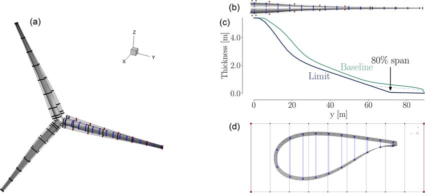
M. H. Aa. Madsen et al.: Multipoint high-fidelity CFD-based aerodynamic shape optimization                                                                                                          167

Table 1. Overview of related work using the adjoint method.

     Reference                                          Turbineg                 Adjoint              Dim.            Ref         Mesh sizea         Design variables           Iterationsb
     Ritlop and Nadarajah (2009)                        –                        Discrete             2-D        2.0 × 10⁶        3.3 × 10⁴                         385            100–200
     Khayatzadeh and Nadarajah (2011)                   –                        Discrete             2-D        2.1 × 10⁶        1.3 × 10⁵                         385                  –
     Schramm et al. (2014)                              –                        Continuous           2-D        3.0 × 10⁶        5.5 × 10⁴                         720                  –
     Schramm et al. (2016)                              –                        Continuous           2-D        7.9 × 10⁶        –                                 480                  –
     Barrett and Ning (2016)                            –                        Continuousf          2-D        1.0 × 10⁶        1.4 × 10⁴                       10–22                  –
                                                                                                                                                               (Table 2)
     Vorspel et al. (2017)                              –                        Continuous           2-D        5.0 × 10⁴        5.0 × 10⁴                       2–364                      –
                                                                                                                                                               (Table 1)
     Schramm et al. (2018)                              –                        Continuous           2-D        2.0 × 10⁶        2.1 × 10⁵                       20–50               0–30
                                                                                                                                                                                (Figs. 5, 7)
     Barrett and Ning (2018)                            –                        Continuousf          2-D        1.0 × 10⁶        1.4 × 10⁴                       10–68                    –
                                                                                                                                                               (Table 1)
     Economon et al. (2013)                             –                        Continuous           2-D        1.0 × 10³        3.2 × 10⁴                          50                 10
                                                        NREL Phase VI                                 3-D        1.0 × 10⁶        7.9 × 10⁶                          84                   3
     Vorspel et al. (2016)                              –                        Continuous           2-D        5.0 × 10⁴        –                                    2        30 (Fig. 3)
                                                        –                                             3-D        1.2 × 10⁶        2.4 × 10⁶                            –       < 8 (Fig. 6)
     Dhert et al. (2017)                                NREL Phase VI            Discrete             3-D        1.0 × 10⁶        2.6 × 10⁶d                      1–252              9–23
     Vorspel et al. (2018)                              NREL Phase VI            Continuous           3-D        1.0 × 10⁶        5.2 × 10⁶e                        5–9        < 8 (Fig. 5)
     Tsiakas et al. (2018)                              MEXICO                   Continuous           3-D        1.0 × 10⁶        2.5 × 10⁶c                        135         10 (Fig. 4)
     This study                                         IEA                      Discrete             3-D        1.0 × 10⁷        1.4 × 10⁷                       1–154           100–200
    a Number of cells in largest mesh used for optimization. b Not all papers state the number of optimization iterations explicitly. In some cases, we report the number of iterations estimated
    from the cited figures. As mentioned in Vorspel et al. (2017), this number depends on the optimization problem and optimizer settings, meaning that cross-setup comparison is difficult.
    c Tsiakas et al. (2018) only gives the number of mesh nodes. d Reduced geometry where the root section was removed. e Applied symmetric boundary conditions (BCs) double the mesh
    size compared to others. f In cases where a range of Reynolds numbers were used, we report the maximum values. g We only found high-fidelity shape optimization for three turbine
    configurations in the literature: two smaller turbines – NREL Phase VI and MEXICO (Schepers et al., 2012) – and the large, commercial-scale IEA 10 MW wind turbine. We find it
    reasonable to assume that the simulations for NREL Phase VI and MEXICO have a Reynolds number on the order of Re = 106 (Sørensen et al., 2002, p. 152; Schepers et al., 2012, p. 10),
    while we estimate the Reynolds number for the IEA turbine to be on the order of Re = 107 (Bak et al., 2013, p. 15–16).

work that included the cited improvements, where they at-                                             been other efforts in turbine blade design using 2-D RANS
tempted to postpone the onset of transition. They concluded                                           CFD with the adjoint method (Barrett and Ning, 2016, 2018)
that both the capability and accuracy of the discrete adjoint                                         that used the open-source compressible solver SU2 (Palacios
optimization framework improved by including the new ad-                                              et al., 2013). These works couple the 2-D RANS and ad-
joint variables for the transition model.                                                             joint model to BEM, panel, and beam element analysis codes
   There have been several contributions to 2-D RANS                                                  to arrive at a 3-D multi-fidelity and multidisciplinary design
shape optimization that use the continuous adjoint approach                                           framework.
(Schramm et al., 2014, 2015, 2016, 2018). In these efforts,                                              Vorspel et al. (2017) present a benchmark of different op-
the continuous adjoint implemented for ducted flows in the                                            timization algorithms (Nelder–Mead, steepest descent, and
flow solver OpenFOAM (Weller et al., 1998) was extended to                                            quasi-Newton) for unconstrained shape optimization in 2-D,
handle external aerodynamics. First, Schramm et al. (2014)                                            where the continuous adjoint solver within OpenFOAM is
optimized the lift-to-drag ratio of the DU 91-W2-250 profile                                          used. The benchmark optimization problem is to find a target
using 720 design variables while constraining cross-sectional                                         lift coefficient from any baseline shape. However, they both
area. They use the “frozen turbulence” assumption, which                                              consider computation time and ease of use to grade the al-
means that no adjoint equation is used for the turbulence                                             gorithms. As already mentioned, they point to the use of the
model. Since each surface point in this work is a design vari-                                        adjoint method to compute the gradient for a large number of
able, they smooth the gradient for stability. The result is a                                         design variables. They recommend that further analysis be
5.7 % to 59 % increase in lift-to-drag ratio for angles of at-                                        done within constrained optimization and within multidisci-
tack ranging from 6.15 to 9.66◦ .                                                                     plinary optimization.
   In a later work, Schramm et al. (2015, 2016) presented                                                In a more recent work within unconstrained optimization,
a finite-difference verification of the adjoint gradients. The                                        Schramm et al. (2018) investigated the effect of the “frozen
same group performed the shape optimization of an upstream                                            turbulence” assumption in 2-D. They carried out their inves-
leading edge (LE) slat for the DU 91-W2-250 airfoil and a                                             tigations on the NACA 0012 and DU 93-W-210 airfoils. In
validation of the framework using wind tunnel data, show-                                             this single-point study, they concluded that the implementa-
ing good agreement below stall (Schramm et al., 2016). The                                            tion of adjoint turbulence models results in better gradients
optimization, which used 480 design variables, resulted in a                                          than those obtained through the frozen turbulence assump-
2 % decrease in drag. As mentioned previously, there have

www.wind-energ-sci.net/4/163/2019/                                                                                                         Wind Energ. Sci., 4, 163–192, 2019
168                             M. H. Aa. Madsen et al.: Multipoint high-fidelity CFD-based aerodynamic shape optimization

tion. Finally, they specifically mention thickness constraints       Table 2. Overview of differences between the work by Dhert et al.
as a future work topic.                                              (2017) and the present work.
   OpenFOAM with a continuous adjoint solver has also
been used in 3-D. This was done by Vorspel et al. (2016),                                       Dhert et al. (2017)   Present work
who first performed a 2-D test case with two design vari-             Geometry                  Reduced geometry      Entire geometry
ables. The 3-D test case consisted of an extruded airfoil with                                  (no root)             included
a spanwise length of five chords and a mesh of 2.4 × 10⁶              Adjoint derivatives       Forward AD            Reverse AD
cells with an y + of 2.5. They investigated both a twist and a        Convergence               [10−1 , 10−2 ]        [10−2 , 10−7 ]
bend–twist coupling case but found that the bending had no            of optimization
discernible effect. This is something they expect to change           Optimization iterations   O(101 )               O(102 )
for future rotating blades applications.                              Maximum mesh size         2.60                  14.16
   The above work does not model the rotation, which is im-           (million)
portant to get the correct local angle of attack along the blade
and thus accurately compute the forces acting on the blade.
Several 3-D adjoint-based optimization efforts model rota-           the adjoint implementation that was used. As we will explain
tion effects, three of which studied the NREL Phase VI rotor         in more detail later (in Sect. 3.2.2), our adjoint implemen-
(Economon et al., 2013; Dhert et al., 2017; Vorspel et al.,          tation uses the automatic differentiation (AD) technique to
2018), and another which studied the MEXICO rotor (Tsi-              compute certain derivatives (Mader et al., 2008). One ma-
akas et al., 2018). Economon et al. (2013) used a continu-           jor improvement is that we implemented the more memory-
ous adjoint formulation to perform single-point aerodynamic          efficient reverse automatic differentiation. Dhert et al. (2017)
shape optimization using a compressible RANS model. In               was forced to use the less memory-efficient forward auto-
2-D, they reduced drag starting from a NACA 4412 pro-                matic differentiation because the reverse option did not in-
file baseline by 4.86 % under imposed thickness constraints.         clude the rotating terms required to model wind turbine ro-
They used a total of 50 design variables and completed 10 de-        tors. We also added constraints on maximum thrust and flap-
sign iterations. In 3-D, they improved the torque coefficient        wise bending moment to align with the IEA case study and
on a mesh with 7.9 million cells by 4 % using 84 shape vari-         enlarged the design space to include chord design variables.
ables with no constraints imposed on geometry or loads. The          Furthermore, Dhert et al. (2017) carried out their studies on
free-form deformation (FFD) box covered part of the blade            the turbine blade excluding the root because of flow solu-
such that both the trailing edge and the innermost part of the       tion convergence issues, whereas we include the root. This
blade could not deform.                                              was made possible by the robustness of the new approxi-
   The optimization was not fully converged, as only three           mate Newton–Krylov (ANK) solver in ADflow, which also
design iterations were performed. One drawback in this early         increases its speed (Yildirim et al., 2018). Finally, we achieve
work is the use of the frozen turbulence assumption, which           an optimality convergence tolerance that is up to 5 orders of
they also identified as an area of future work.                      magnitude lower.
   Dhert et al. (2017) used a discrete adjoint solver to carry          Another recent effort is that of Vorspel et al. (2018),
out a multipoint optimization of a two-bladed rotor using a          who performed unconstrained optimization of the NREL
2.6 million cell mesh, where they maximized the torque co-           Phase VI rotor where they minimized the thrust by varying
efficient using up to 252 design variables. They used pitch,         up to nine twist design variables using a steepest descent op-
twist, and local shape design variables while constraining the       timization algorithm. Not surprisingly, they mention conver-
thickness between 15 % and 50 % of the local blade chord to          gence issues, in part due to the turbine being stall regulated
ensure adequate space for a structural box. The final multi-         and exhibiting separated flow at some inflow speeds. Vortices
point optimization resulted in a 22.1 % increase in torque co-       at tip and root further impaired the convergence, which in
efficient but also increased the thrust by 69 %. The original        turn resulted in poor gradient quality. They addressed this is-
design was meant to be a three-bladed rotor, which explains          sue by limiting the deformable area to only the outer 50 %
the low thrust coefficients in the reported results (Dhert et al.,   of the blade length, which limited the shape design opti-
2017, Table 1). They found the optimized shapes for both sin-        mization. Like Economon et al. (2013), they used the frozen
gle and multipoint optimization exhibited highly cambered            turbulence assumption. However, they differed in choice of
trailing edges at the root region where the wind speed is re-        turbulence model: Vorspel et al. (2018) used the k − ω SST
duced. While this does agree with what has been reported             model, while Economon et al. (2013) used the SA turbulence
in 2-D cases (Ritlop and Nadarajah, 2009), it is also exactly        model. For future work, they suggested the use of more ef-
what one would expect when chord is not included as a de-            ficient optimization algorithms, and mentioned the inclusion
sign variable.                                                       of the adjoint turbulence equations and the study of turbines
   The present work builds on Dhert et al. (2017), who used          that are not stall regulated.
the same CFD solver, ADflow. Our improvements are sum-
marized in Table 2. One major improvement has to do with

Wind Energ. Sci., 4, 163–192, 2019                                                          www.wind-energ-sci.net/4/163/2019/
M. H. Aa. Madsen et al.: Multipoint high-fidelity CFD-based aerodynamic shape optimization                                                                                                169

Table 3. Overview of aerodynamic optimization works of wind turbine rotors using the adjoint method.

                                                 Turbu-          Deformation                Geometry          Load constraints           Geometric              Design variables
   Reference                          Multi
                                                   lence      (X= full blade)        (X= full blade)         Thrust       Moment         constraints       Twist      Chord       Shape
   Economon et al. (2013)                                                                              X                                            X                                  X
   Dhert et al. (2017)                    X            X                                                                                            X          X                       X
   Vorspel et al. (2018)                                                                               X                                                       X
   Tsiakas et al. (2018)                               X                      X                        X                                                                               X
   This study                             X            X                      X                        X           X              X                 X          X           X           X
  Multi: multipoint optimization; turbulence: whether the turbulence model is included in the adjoint solver; deformation: whether the entire blade was allowed to deform; geometry: whether
  the entire blade was modeled; geometric constraints: whether any geometric constraints were imposed.

   Finally, Tsiakas et al. (2018) used a continuous adjoint                                        In Table 3, the present work is compared to the above-cited
approach that included the SA turbulence equations to op-                                          3-D shape optimization efforts on wind turbine rotors.
timize the MEXICO RWT. The flow was modeled by the                                                    As previously mentioned, structural considerations are
incompressible RANS equations and solved in a co-moving                                            crucial in wind turbine design. Anderson et al. (2018) par-
frame of reference. They maximized the power for a single                                          tially addressed this issue by coupling the NSU3D RANS
wind speed of 10 m s−1 . Compared to the present work, they                                        solver with the AStrO structural finite element solver through
used a different parameterization technique based on volu-                                         a fluid–structure interface to converge on realistic, steady-
metric non-uniform rational B splines (NURBS), which con-                                          state loads on the SWiFT RWT. They used Abaqus to make
fine the blade in a small volume. NURBS are used both for                                          a finite element model with shell elements. They performed
the deformation of the surface and the volume meshes, and                                          a purely structural optimization of the composite blade, with
the outermost NURBS control points are fixed to keep the                                           the loads computed by the CFD. The optimization’s objec-
outer volume mesh fixed. This only ensures C 0 continuity.                                         tive was to, using gradient-based optimization, minimize the
They use 385 NURBS, resulting in 135 design variables,                                             off-axis stress with respect to 16 310 ply orientation vari-
which are only allowed to move in the direction perpendicu-                                        ables. They completed 10 optimization iterations consider-
lar to the rotor plane. This choice of parameterization limits                                     ing five different load cases and achieved a reduction in the
the design space; for example, no chord increase can be ob-                                        maximum fatigue stress between 40 % and 60 %. They did
tained without simultaneously changing profile shape. The                                          so without adding any constraints, but they did assume the
flow and adjoint solvers take advantage of graphics process-                                       material to be a single-ply, unidirectional fiber composite for
ing unit (GPU) hardware, resulting in fast solutions. Indeed,                                      each blade section. The logical next step would be to per-
they state that the overall optimization process can run up to                                     form the simultaneous optimization of the structural sizing
50 times faster on GPUs than on CPUs. They obtained a 3 %                                          and aerodynamic shape optimization, as is already done in
increase in the objective function and attribute this modest                                       aircraft wing design (Kenway and Martins, 2014).
improvement to the limited freedom in the parameterization.
   In spite of the contributions cited above, many improve-
ments are needed before we achieve the ultimate goal of pro-                                       3    Methodology
viding a “push-button solution” for wind turbine manufac-
turers. This paper contributes with some of these improve-                                         We now briefly describe all components of the optimization
ments by including all of the following features in a compre-                                      framework. The overall workflow is shown in Fig. 1 using an
hensive high-fidelity 3-D RANS-based shape optimization                                            extended design structure matrix (XDSM) diagram (Lambe
framework:                                                                                         and Martins, 2012). An initial set of design variable val-
                                                                                                   ues, x (0) , is given to the optimizer. The optimizer passes the
  1. enforcement of geometric constraints to ensure struc-                                         current design variables to the surface deformation module,
     tural feasibility,                                                                            prompting it to update the surface mesh (except for the very
                                                                                                   first iteration). The surface deformation module also pro-
  2. normal operation rotor load constraints limiting thrust
                                                                                                   vides analytic derivatives of the surface mesh with respect
     and flapwise bending moment,
                                                                                                   to the design variables, dx s /dx. After the surface mesh has
  3. more precision and stability in the convergence of flow                                       been updated, it is passed to the volume deformation mod-
     and adjoint solvers,                                                                          ule, which updates the volume mesh and computes its ana-
                                                                                                   lytic derivatives with respect to the surface mesh, dx v /dx s .
  4. inclusion of a turbulence model in the adjoint solver,                                        Then, the flow solver computes the flow states, w. These
  5. a comprehensive set of design variables, and                                                  states are passed to the adjoint solver, which computes the to-
                                                                                                   tal derivative. Finally, the objective function, f (e.g., torque),
  6. modeling and deformation of the entire blade shape.                                           as well as its derivatives, df/dx, are provided to the opti-

www.wind-energ-sci.net/4/163/2019/                                                                                                    Wind Energ. Sci., 4, 163–192, 2019
170                           M. H. Aa. Madsen et al.: Multipoint high-fidelity CFD-based aerodynamic shape optimization

mizer, which computes a new step for another optimization         good agreement was found. EllipSys3D has also been com-
iteration. Both the surface and volume deformation steps are      pared with OpenFOAM for a case with atmospheric flow
fast explicit operations. On the other hand, the flow and ad-     over complex terrain. EllipSys3D was found to be 2–6 times
joint solvers are costly iterative operations that take up the    faster while producing almost identical numerical results
vast majority of the computation time. The optimization pro-      (Cavar et al., 2016). More recent sources also show that these
cess involves O(102 ) major iterations, which is an absolute      two solvers yield comparable results (Sørensen et al., 2016;
minimum bound on the number of CFD solutions and mesh             Yilmaz et al., 2017; Boorsma et al., 2018).
updates; there are additional CFD solutions within each ma-
jor iteration.                                                    3.2.2   ADflow
                                                                  ADflow is a compressible RANS solver based on SUmb
3.1     Geometry and mesh deformation                             (Weide et al., 2006), a structured FVM CFD solver written in
                                                                  Fortran 90 that uses cell-centered variables on a multi-block
To deform the surface geometry and mesh, we use the Python
                                                                  grid. Unlike EllipSys3D, ADflow uses the Spalart–Allmaras
module pyGeo developed by Kenway et al. (2010), which
                                                                  (SA) turbulence model (Spalart and Allmaras, 1994) and
implements the FFD (Sederberg and Parry, 1986) technique.
                                                                  works with state variables computed using the Jameson–
Some of the key features of FFD are analytic derivatives and
                                                                  Schmidt–Turkel (JST) scheme. More recently, Kenway et al.
a machine-precision representation of the baseline geometry.
                                                                  (2017) implemented overset mesh capability. ADflow is
   The volume deformation tool is called IDWarp and is
                                                                  wrapped with Python to provide a more convenient user in-
based on the inverse distance weighting function (Edward
                                                                  terface and to facilitate integration with optimization algo-
et al., 2012). IDWarp is a fast and unstructured deformation
                                                                  rithms and other components of an MDO framework.
algorithm that has been demonstrated in aerodynamic (Yu
                                                                     ADflow has been coupled to a structural finite element
et al., 2018; He et al., 2018) and aerostructural applications
                                                                  solver in the MACH (MDO for aircraft configurations with
(Brooks et al., 2018).
                                                                  high fidelity) framework (Kenway et al., 2014), which has
                                                                  been used to perform not only aerostructural optimization of
3.2     Flow and adjoint solvers                                  aircraft configurations (Kenway and Martins, 2014; Brooks
                                                                  et al., 2018; Burdette and Martins, 2018, 2019) but also hy-
3.2.1    EllipSys3D                                               drostructural optimization of hydrofoils (Garg et al., 2019,
EllipSys3D is an in-house, structured, multi-block, finite vol-   2017).
ume method (FVM) flow solver developed at DTU Wind En-               As previously mentioned, we use an ANK solver, which
ergy by Michelsen (1992, 1994) and Sørensen (1995), and           is implemented in ADflow to provide robustness. The ANK
we use it in the present work to perform the comparison be-       implementation is important since it is crucial to properly
tween CFD solvers. It discretizes the incompressible RANS         converge the flow field in order to obtain accurate gradi-
equations using general curvilinear coordinates and couples       ents. Newton–Krylov (NK) methods are not robust because
velocity and pressure through the SIMPLE algorithm.               they might not converge if the starting point is outside the
   In this study, we run EllipSys3D using the third-order         basin of attraction. ANK addresses this convergence issue
quadratic upwind interpolation for convection kinematics          using a globalization method called pseudo-transient con-
(QUICK) scheme and the k−ω SST (Menter, 1993) model to            tinuation, which starts with the stable but inefficient back-
calculate the turbulent eddy viscosity, which compares favor-     ward Euler method with a small time step, and then increases
ably to other turbulence models for wind turbine applications     the time step to approach the higher convergence rate of
(Reggio et al., 2011).                                            the NK solver. The ANK method involves the solution of
   EllipSys3D has been validated against experimental data        large linear systems using preconditioners. These systems are
for the MEXICO RWT (Bechmann et al., 2011) and the                solved in a matrix-free fashion with the generalized minimal
NREL Phase VI RWT (Sørensen et al., 2002; Sørensen and            residual (GMRES) algorithm (Saad and Schultz, 1986) using
Schreck, 2014), and also in a blind comparison (Simms et al.,     the Portable, Extensible Toolkit for Scientific Computation
2001). In addition, the unsteady interaction between tower        (PETSc) library (Balay et al., 2018a, b, 1997). The adjoint
and blade has been simulated for the NREL Phase VI RWT            solver linear systems are solved using the same algorithm.
with EllipSys3D using overset grid capabilities, and an over-     ADflow is considered converged when the ratio of the L2
all good agreement was found with experimental data (Zahle        norm of the residuals at iteration n and the same norm of the
et al., 2009). EllipSys3D has been used in various rotor ap-      free stream residual is below a given tolerance, i.e., when
plications to perform computations, such as aerodynamic                kRn k2
power (Johansen et al., 2009) and fluid–structure interac-        η≤          .                                              (1)
                                                                        Rfs 2
tion (Heinz et al., 2016). The latter work also encompasses
a comparison across fidelities between the CFD-based tool,        For the optimizations presented below, we typically set η =
HAWC2CFD, and the BEM-based HAWC2 solvers where a                 10−9 , whereas the L2 convergence for the adjoint equation

Wind Energ. Sci., 4, 163–192, 2019                                                      www.wind-energ-sci.net/4/163/2019/
M. H. Aa. Madsen et al.: Multipoint high-fidelity CFD-based aerodynamic shape optimization                                                171

Figure 1. Extended design structure matrix (XDSM) showing the optimization framework. Green blocks are iterative solvers, whereas red
boxes represent explicit functions. Black lines represent the process flow in the order of the numbers; gray lines represent data dependencies.

is set to 10−7 . These convergence thresholds are not to be               to obtain
confused with the optimality tolerance, which we set to 10−4 .
                                                                                    ∂f ∂R −1 ∂R

   One crucial capability in ADflow is the efficient computa-             df   ∂f
                                                                             =    −               ,                                        (4)
tion of gradients through its adjoint solver. Together with the           dx   ∂x ∂w ∂w        ∂x
                                                                                    |   {z   }
geometry and mesh deformation tools mentioned above, and                                      9T
the optimization software mentioned in the next section, this
enables aerodynamic shape optimization with respect to hun-               where we have only partial derivative terms that can be found
dreds of design variables (Lyu et al., 2014; Chen et al., 2016;           analytically at a low computational cost. The linear system in
Dhert et al., 2017). All the optimization results in Sect. 6 are          this equation can either be solved by computing the solution
obtained with the ADflow framework.                                       Jacobian, dw/dx, from the linear system from Eq. (3) or by
   We now derive the adjoint equations and briefly explain                solving the adjoint system:
how they are assembled and solved. A detailed description
                                                                            ∂R T           ∂f T

of the implementation is provided in previous work (Mader                         9=             ,                                   (5)
et al., 2008; Mader and Martins, 2011; Lyu et al., 2013). The               ∂w            ∂w
CFD solver computes the flow field, w, for a given set of
                                                                          where 9 is the adjoint vector, which can be substituted into
design variables, x, by converging the residuals R(x, w) of
                                                                          the total derivative equation (Eq. 2), i.e.,
the governing equations to zero. Then, any function of in-
terest, f (x, w), can be computed. Gradient-based optimizers              df   ∂f      ∂R
require the gradient of the objective and constraint functions               =    − 9T    .                                                (6)
                                                                          dx   ∂x      ∂x
with respect to the design variables. To compute this gradi-
ent, we use the equation for the total derivative:                           The cost of the adjoint method is independent of the num-
                                                                          ber of design variables because the adjoint equation (Eq. 5)
df   ∂f   ∂f dw                                                           does not contain x. However, if there are multiple functions
   =    +       .                                                (2)
dx   ∂x ∂w dx                                                             of interest f , we need to solve Eq. (5) for each f with a dif-
Here, the partial derivatives correspond to derivatives of ex-            ferent right-hand side. Given that our problem has O(102 )
plicit functions, while the total derivative involves the iter-           design variables and only a few functions of interest, the ad-
ative solution of the governing equations. Thus, the partial              joint method is particularly advantageous.
derivatives can be found analytically at a low computational                 In the adjoint equation (Eq. 5) and total derivative equa-
cost, but the direct computation of the total derivative dw/dx            tion (Eq. 6), we need to provide two matrices and two vectors
should be avoided. A similar total derivative equation can be             of partial derivatives. As mentioned above, these derivatives
written for the residuals, which must remain zero for the CFD             involve only explicit operations and are in principle cheap
solution to hold, and thus                                                to compute. However, they still require the differentiation of
                                                                          parts of a complex CFD code, and a good implementation
dR ∂R ∂R dw
   =   +      = 0.                                               (3)      is essential to preserve the accuracy and efficiency of the ad-
dx   ∂x ∂w dx                                                             joint approach. Traditionally, adjoint method developers have
We can now substitute the solution of the Jacobian given by               derived these partial derivatives by differentiating the equa-
the above equation into the total derivative equation (Eq. 2)             tions or code manually and programming new functions that

www.wind-energ-sci.net/4/163/2019/                                                                  Wind Energ. Sci., 4, 163–192, 2019
172                            M. H. Aa. Madsen et al.: Multipoint high-fidelity CFD-based aerodynamic shape optimization

compute those derivatives. This process is labor intensive          4     Flow solver comparison
and prone to programming errors. To address this drawback,
Mader et al. (2008) pioneered the use of automatic differen-        In this work, we use ADflow as the CFD solver in the design
tiation to compute the partial derivatives. Automatic differ-       optimization due to its adjoint gradient computation and inte-
entiation is a technique that takes a given code and produces       gration with geometry parameterization, mesh deformation,
new code that computes the derivatives of the outputs with          and optimization tools. However, EllipSys3D has been more
respect to the inputs (Griewank, 2000). Using a pure auto-          thoroughly validated for wind turbine rotor flows, so in this
matic differentiation approach to compute our derivatives of        section, we verify ADflow against EllipSys3D for a three-
interest, df/dx, would mean applying the automatic differ-          bladed pitch-regulated rotor geometry. In this section, we
entiation tool to the whole CFD code, including the iterative       only include a mesh convergence study for one operational
solver. While this produces accurate derivatives, it is not an      condition. A more detailed flow comparison is included in
efficient approach. By selectively using automatic differenti-      Appendix A.
ation to produce code that computes only the partial deriva-
tives, which do not involve the iterative solver, we lower the      4.1    Fluid model and computational mesh
adjoint implementation effort while keeping the efficiency of
the traditional adjoint implementation approach. There are          All simulations are steady-state 3-D RANS of the rotor only,
still many details involved in making our adjoint implemen-         where effects from both tower and nacelle have been ne-
tation approach efficient; these details have been presented in     glected. Since we study a rigid upwind turbine, neglecting
previous work (Mader et al., 2008; Lyu et al., 2013).               tower and nacelle should have a limited effect. We also note
   As briefly mentioned in the introduction, there are two          that we compute the flow field using a co-rotating, non-
modes for automatic differentiation: the forward mode and           inertial reference frame that is attached to the rotor. There-
the reverse mode. Dhert et al. (2017) had used automatic dif-       fore, the RANS equations have additional terms to account
ferentiation in forward mode to compute and store the flow          for Coriolis and centripetal forces. Just as for the IEA Wind
Jacobian, ∂R/∂w, as well as the other partial derivatives.          Task 37 case, the three-bladed pitch-regulated rotor geome-
Then, these stored matrices are used by the adjoint solver          try in the analysis is a design based on the DTU 10 MW RWT
to compute transpose-matrix-vector products to converge the         (Bak et al., 2013), where both chord and twist distributions
adjoint solution, 9. Using the reverse mode, no storage of the      have been altered to allow for more room for improvement
Jacobian is needed. Instead, a matrix-free approach is used,        using design optimization. We compare the twist and thick-
where the transpose-matrix-vector products required to con-         ness distributions for the DTU 10 MW RWT and the IEA
verge the adjoint solution are computed directly through the        Wind Task 37 baseline in Fig. 2
reverse mode derivative routines. While the reverse mode is            The surface mesh consists of three blades, each with 36
more efficient in terms of memory usage, the reverse mode           blocks. For each blade, there are 256 cells in the chordwise
implementation was missing the rotation terms required for          direction and 128 in the spanwise direction (tip excluded).
wind turbine modeling. We have fixed this for the implemen-         The surface mesh is generated using the in-house Parametric
tation in the present work and use the reverse mode instead.        Geometry Library (PGL). The tip was constructed using four
The implemented reverse AD routines may also lead to speed          blocks of 32 × 32 cells each, resulting in a total surface mesh
up depending on the number of Krylov iterations needed to           with 110 592 mesh cells.
converge the adjoint system.                                           The spherical volume mesh has an O–O topology gener-
                                                                    ated with the hyperbolic in-house mesh generator HypGrid
                                                                    (Sørensen, 1998). Setting the first boundary layer cell height
3.3   Optimizer
                                                                    to 10−6 m yields a y + of around 1 for the given operational
We use the Sparse Nonlinear OPTimizer (SNOPT) (Gill                 conditions, and a total of 128 cell layers are grown from
et al., 2002) for all optimizations herein. SNOPT imple-            the surface mesh where the farthest vertices reach a distance
ments a sequential quadratic programming (SQP) algorithm.           of 1740 m. This results in a total of 432 blocks, each with
We use it through the open-source Python wrapper py-                32 × 32 × 32 cells, which is equivalent to 14.155776 million
OptSparse4 , which provides a common interface to this and          cells. Given a span of R = 89.166 m, the surrounding spher-
other optimization software. The convergence in SNOPT is            ical mesh expands to about 20 times the blade span.
set through the “major optimality tolerance” setting (Gill             The mesh we just described above is the finest mesh we
et al., 2007). We aim at converging all optimization problems       use, which we call the L0 mesh. A coarser (L1) mesh is ob-
to 10−4 .                                                           tained by coarsening L0 once, i.e., by removing every second
                                                                    cell in all three directions. Similarly, the L2 mesh is obtained
                                                                    by coarsening L1. Unless otherwise stated, we use these three
                                                                    meshes in all the work herein. The turbine geometry and the
   4 https://github.com/mdolab/pyoptsparse (last access: 18 March   surrounding spherical mesh are shown in Fig. 3, and a more
2019)                                                               detailed view of the rotor is shown in Fig. 4.

Wind Energ. Sci., 4, 163–192, 2019                                                         www.wind-energ-sci.net/4/163/2019/
M. H. Aa. Madsen et al.: Multipoint high-fidelity CFD-based aerodynamic shape optimization 173
Figure 2. Comparison of chord (a) and twist (b) for the DTU 10 MW RWT and the perturbed design used as the starting point for the IEA
optimization case study. Both the chord and twist are reduced. The baseline blade design is based on the FFA-W3 airfoil family with relative
thicknesses in the range of [24 %, 36 %].
Figure 4. Baseline geometry used in the flow solver comparison
and as starting point for the optimization. Each blade has a surface
mesh with 36 square blocks. Each block has 32 × 32 cells, resulting
in 110 592 surface mesh cells.
Figure 3. The baseline wind turbine design with the spherical L0
mesh around it. The blade span is 89.166 m, and the spherical mesh solution on mesh L0. This agrees with an earlier mesh con-
stretches to 20 times the blade span. vergence study (Dhert et al., 2017, Table 1), where up to
22 million cells were used without reaching convergence.
Therefore, we generated a finer mesh with more than 47 mil-
4.2 Mesh convergence study lion cells called L-1. The L-1 mesh is made exclusively for
the present grid convergence study and will not be used in
To quantify the mesh dependence for each solver, we com- the ensuing optimizations.
pute the integrated metrics – torque and thrust – for the three Table 4 shows that error reduction from L0 to L-1 for AD-
mesh levels (L0, L1, and L2) and list them in Table 4. The flow is much lower (with reductions of about 4 % in thrust
operational condition corresponds to a wind speed of 8 m s−1 and 7 % in torque) than the error reduction from L2 to L1
and rotor speed of 6.69 rpm at zero blade pitch, which is one (15 % and 21 %) or from L1 to L0 (22 % and 41 %). The er-
of the conditions listed in Table A1 in Appendix A. As is ev- rors are computed using the Richardson extrapolation values
ident from the results for meshes L2, L1, and L0 in Table 4, from Fig. 5, which are based on an estimate of the contin-
ADflow does not produce a sufficiently mesh-independent uum value (in the limit of an infinitely fine mesh), given by
www.wind-energ-sci.net/4/163/2019/ Wind Energ. Sci., 4, 163–192, 2019174 M. H. Aa. Madsen et al.: Multipoint high-fidelity CFD-based aerodynamic shape optimization
Figure 5. Richardson extrapolation (Eq. 7) for the grid convergence study for thrust (a) and torque (b). Between the two solvers, the
extrapolated continuum values for thrust differ by 3 %, whereas the errors for the torque values vary by less than 0.7 %.
Table 4. Mesh convergence study for the compressible solver ADflow and the incompressible solver EllipSys3D. The operational conditions
for the convergence study correspond to the 8 m s−1 case listed in Table A1. The error percentages are estimated using the Richardson
extrapolations from Fig. 5.
ADflow EllipSys3D
Mesh Cells Thrust Error Torque Error Thrust Error Torque Error
(million) (kN) (%) (kNm) (%) (kN) (%) (kNm) (%)
L2 0.221 934 58.6 10 403 134.5 584 2.1 4336 3.2
L1 1.769 733 24.4 6156 38.3 578 1.0 4402 1.7
L0 14.155 625 6.1 4877 9.6 573 0.2 4457 0.5
L-1 47.776 603 2.4 4547 2.2 577 0.9 4471 0.2
Extrapolation ∞ 589 0.0 4451 0.0 572 0.0 4475 0.0
Roache (1994): tained with L2 throughout the presented work to substantiate
this claim.
f1 − f2 There is a slight increase in error for EllipSys3D in the
fc ≈ f1 + , (7) thrust value on the finest mesh level, which is unexpected. It
r2 − 1
is also surprising that the compressible solver seems to bene-
where fc is the continuum value, f1 and f2 are the values fit so drastically from an increase in cell count. Recent stud-
obtained using the L0 and L1 meshes, respectively, and r is ies have suggested this can be the case for some compress-
the grid refinement ratio. ible solvers (Sørensen et al., 2016). From the expressions
In Table 4, we can also see that the two solvers tend to con- for the Prandtl–Glauert compressibility corrections (Glauert,
verge towards the same thrust and torque continuum values 1928), one would expect that compressible effects could be
– 0.3 % difference for thrust and 0.7 % difference for torque. at play, which agrees with our results. Compressibility ef-
Based on the results in this table, we determine that the L0 fects in wind turbine applications have become increasingly
mesh represents a reasonable compromise between accuracy significant as turbine rotor sizes have increased. One of the
(less than 10 % error) and speed. conclusions from the AVATAR project was that compressibil-
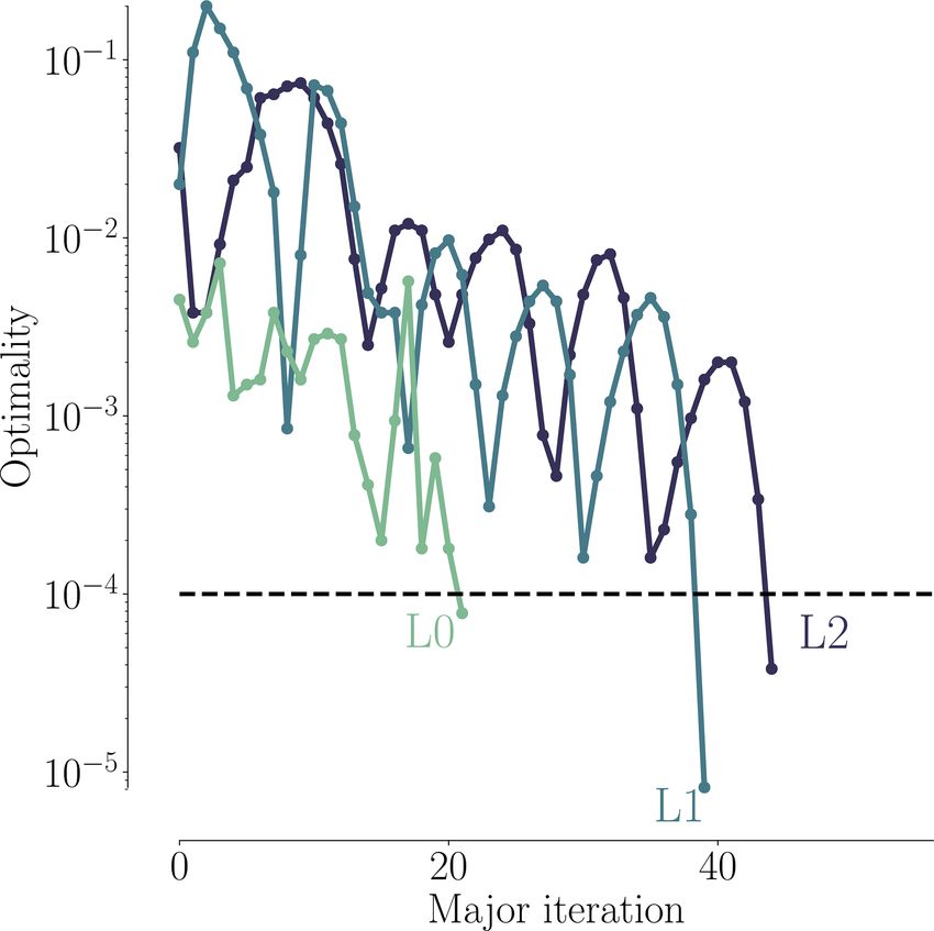
It is clear from Fig. 5 that mesh level L2 is very coarse and ity effects play a role in large wind turbines (Sørensen et al.,
yields very different results. As we will demonstrate later, the 2017, p. 9). In the AVATAR project, results from EllipSys3D
suggested design trends from such a coarse mesh can some- were compared to results from a compressible CFD code.
times lead to savings in computation time and, other times, Here, they studied a case with an inflow speed of 14 m s−1
lead to completely wrong design trends. Thus, one should and a Mach number of 0.2457 (Sørensen et al., 2017, Fig. 8),
use such coarse meshes with care. We report the results ob- where the obtained Cp curves differed in particular on the
Wind Energ. Sci., 4, 163–192, 2019 www.wind-energ-sci.net/4/163/2019/You can also read