Ensemble-based statistical interpolation with Gaussian anamorphosis for the spatial analysis of precipitation - NPG
←
→
Page content transcription
If your browser does not render page correctly, please read the page content below
Nonlin. Processes Geophys., 28, 61–91, 2021
https://doi.org/10.5194/npg-28-61-2021
© Author(s) 2021. This work is distributed under
the Creative Commons Attribution 4.0 License.

Ensemble-based statistical interpolation with Gaussian
anamorphosis for the spatial analysis of precipitation
Cristian Lussana, Thomas N. Nipen, Ivar A. Seierstad, and Christoffer A. Elo
Norwegian Meteorological Institute, Oslo, Norway

Correspondence: Cristian Lussana (cristianl@met.no)

Received: 10 June 2020 – Discussion started: 19 June 2020
Revised: 10 November 2020 – Accepted: 27 November 2020 – Published: 22 January 2021

Abstract. Hourly precipitation over a region is often simul-         radars, and in situ observations. For this last data source,
taneously simulated by numerical models and observed by              measurements from both traditional and opportunistic sen-
multiple data sources. An accurate precipitation representa-         sors have been considered.
tion based on all available information is a valuable result for
numerous applications and a critical aspect of climate mon-
itoring. The inverse problem theory offers an ideal frame-
work for the combination of observations with a numerical
model background. In particular, we have considered a mod-           1   Introduction
ified ensemble optimal interpolation scheme. The deviations
between background and observations are used to adjust for           Precipitation amounts are measured or estimated simultane-
deficiencies in the ensemble. A data transformation based on         ously by multiple observing systems, such as networks of
Gaussian anamorphosis has been used to optimally exploit             automated weather stations and remote sensing instruments.
the potential of the spatial analysis, given that precipitation is   At the same time, sophisticated numerical models simulating
approximated with a gamma distribution and the spatial anal-         the evolution of the atmospheric state provide a realistic pre-
ysis requires normally distributed variables. For each point,        cipitation representation over regular grids with the spacing
the spatial analysis returns the shape and rate parameters of        of a few kilometers. An unprecedented amount of rainfall
its gamma distribution. The ensemble-based statistical inter-        data is available nowadays at very short sampling rates of
polation scheme with Gaussian anamorphosis for precipita-            1 h or less. Nevertheless, it is a common experience within
tion (EnSI-GAP) is implemented in a way that the covari-             national meteorological services that the exact amount of
ance matrices are locally stationary, and the background er-         precipitation, to some extent, eludes our knowledge. There
ror covariance matrix undergoes a localization process. Con-         may be numerous reasons for this uncertainty. For example,
cepts and methods that are usually found in data assimilation        a thunderstorm triggering a landslide may have occurred in a
are here applied to spatial analysis, where they have been           region of complex topography where in situ observations are
adapted in an original way to represent precipitation at finer       available but not exactly at the landslide spot; thus, weather
spatial scales than those resolved by the background, at least       radars may cover the region in a patchy way because of ob-
where the observational network is dense enough. The EnSI-           stacles blocking the beam, and numerical weather prediction
GAP setup requires the specification of a restricted number          forecasts are likely to misplace precipitation maxima. An-
of parameters, and specifically, the explicit values of the er-      other typical situation is when an intense and localized sum-
ror variances are not needed, since they are inferred from the       mer thunderstorm hits a city. In this case, several observation
available data. The examples of applications presented over          systems are measuring the event and more than one numeri-
Norway provide a better understanding of EnSI-GAP. The               cal model may provide precipitation totals. From this plural-
data sources considered are those typically used at national         ity of data, a detailed reconstruction of the event is possible,
meteorological services, such as local area models, weather          provided that the data agree both in terms of the event inten-
                                                                     sity and on its spatial features. This is not always the case,

Published by Copernicus Publications on behalf of the European Geosciences Union & the American Geophysical Union.
62                                                                       C. Lussana et al.: Spatial analysis of precipitation

and sometimes meteorologists and hydrologists are left with      lar, Jermey and Renshaw (2016) demonstrates that increas-
a number of slightly different but plausible scenarios.          ing resolution via downscaling improves precipitation rep-
   The objective of our study is the precipitation reconstruc-   resentation, though they also point out that assimilating ob-
tion through a combination of numerical model output with        servations at a high resolution in numerical models is im-
observations from multiple data sources. The aim is that the     portant for reconstructing high-threshold/small-scale events.
combined fields will provide a more skillful representation      The sources of model errors and their treatments in data as-
than any of the original data sources. As remarked above,        similation (DA) schemes have been studied extensively. For
any improvement in the accuracy and precision of precipi-        instance, in the introduction of the paper by Raanes et al.
tation can be of great help for monitoring the weather, but      (2015), a list of model errors is reported, together with sev-
it is not only that. Snow- and hydrological- modeling will       eral references to other studies addressing them. Regarding
benefit from improvements in the quality of precipitation,       precipitation forecasts, model errors often encountered in ap-
which is one of the atmospheric forcing variables (Magnus-       plications are (Müller et al., 2017) systematic under- or over-
son et al., 2019; Huang et al., 2019). Climate applications      estimations of amounts, spatial errors in the placement of
that make use of reanalysis (e.g., Hersbach et al., 2020; Jer-   events, and underestimations of uncertainty. With reference
mey and Renshaw, 2016) or observational gridded data sets        to spatial analysis, we consider observed precipitation data
(e.g., Lussana et al., 2018), such as, for instance, the eval-   to be more accurate than model estimates. In fact, model
uation of a regional climate model (Kotlarski et al., 2017)      outputs are evaluated in terms of their ability to reconstruct
or the calculation of climate indices (Vicente-Serrano et al.,   observed values. The most important disadvantage of obser-
2015), may also benefit from data sets combining model           vational networks is that often they do not cover the region
output and observations, as shown by Fortin et al. (2018).       under consideration; moreover, observations may be irregu-
Besides, the intensity–duration–frequency curve (IDF curve)      larly distributed in space and present missing data over time.
derived from precipitation data sets are widely used in civil    Each observational data source has its own characteristics
engineering for determining design values, and the quality of    that have been extensively studied in the literature that we
the reconstruction of extremes has a strong influence on IDF     will address here only superficially, since our objective is
curves (Dyrrdal et al., 2015).                                   the combination of information. For example, rain gauges are
   The data sources considered in our study are precipitation    possibly the most accurate precipitation measurement avail-
ensemble forecasts, observations from in situ measurement        able at present (CIMO, 2014), apart from when the observa-
stations, and estimates derived from weather radars. Numer-      tions are affected by gross measurement errors, as defined by
ical model fields are available everywhere, and the quality      Gandin (1988). There are multiple sources of uncertainty for
of their output is constantly increasing over the years. The     gauge measurements (Zahumensky, 2004), such as catching
weather-dependent uncertainty is often delivered in the form     and counting (Pollock et al., 2014). The undercatch of solid
of an ensemble. At present, assessments using hydrologi-         precipitation due to wind (Wolff et al., 2015) is a signifi-
cal models have shown that input from numerical models           cant problem in cold climates. Radar-derived estimates are
“may be comparable or preferable compared to gauge ob-           affected by several issues such as blocking and nonuniform
servations to drive a hydrologic and/or snow model in com-       attenuation of the radar beam due to obstacles along the path,
plex terrain”, as stated by Lundquist et al. (2019), based on    especially in a complex terrain. A statement in the introduc-
their review of recent research. One of the key messages by      tion of the book by Germann and Joss (2004) is illuminating
Lundquist et al. (2019) is that numerical models represent       in this sense. “To put a weather radar in a mountainous re-
precipitation fields at ungauged sites in a realistic and con-   gion is like pitching a tent in a snowstorm: the practical use
vincing way, as it is demonstrated by the accuracy of their      is obvious and large – but so are the problems” (Germann and
total annual rain and snowfall estimates, notwithstanding that   Joss, 2004). In addition, weather radars do not directly mea-
daily or subdaily aggregated precipitation fields may mis-       sure precipitation; instead, they measure reflectivity, which is
represents individual precipitation events, such as storms. In   then transformed into a precipitation rate. The transformation
the work by Crespi et al. (2019), it has been demonstrated       itself contributes to increasing the uncertainty of the final es-
that the combination of numerical model outputs and in situ      timates. Another important aspect of observational data that
observations improve the representation of monthly precip-       will be treated only marginally here is data quality control.
itation climatologies over Norway, if compared to similar        In this work we will consider only quality-controlled obser-
products based on in situ observations only. Lussana et al.      vations. To sum up, in situ data are the more accurate ob-
(2019b) have successfully used monthly precipitation clima-      servations of precipitation that we will consider. Thus, radar
tologies to improve the performances of statistical interpo-     estimates, which are calibrated using gauges as references,
lation methods in complex terrain over Norway. However,          are less accurate than in situ data. They are spatially corre-
because model fields represent areal averages, the charac-       lated with the actual precipitation, and they are affected by
teristics of simulated precipitation depend significantly on     less uncertainty than the simulations carried out by numeri-
the model resolution, as remarked for global and regional        cal models. Numerical model output is the basic information
reanalyses over the Alps by Isotta et al. (2019). In particu-

Nonlin. Processes Geophys., 28, 61–91, 2021                                          https://doi.org/10.5194/npg-28-61-2021
C. Lussana et al.: Spatial analysis of precipitation                                                                           63

available everywhere and the one we consider more uncer-           general enough to cover a wide range of cases. Our approach
tain.                                                              is to specify the reliability of the background, with respect
   Inverse problem theory (Tarantola, 2005) provides the           to observations, in such a way that error variances can vary
ideal framework for the combination of observations with a         both in time and space. An additionally innovative part of
numerical model background. The marginal distribution of           our research is that we consider opportunistic sensing net-
the precipitation analysis is assumed to be a gamma distribu-      works of the type described by de Vos et al. (2020) within
tion, and we aim at estimating its shape and rate parameters       the examples of the applications proposed. Citizen weather
for each grid point. The gamma distribution is appropriate         stations are rapidly increasing in prevalence and are becom-
for representing precipitation data, as reported, for example,     ing an emerging source of weather information, as described
by Wilks (2019). The formulation of the statistical interpo-       by Nipen et al. (2020). Thanks to those networks, for some
lation method presented is similar to the analysis step of the     regions we can rely on an extremely dense spatial distribu-
ensemble Kalman filter (Evensen, 2006) or the ensemble op-         tion of in situ observations.
timal interpolation (EnOI; Evensen, 2003), with the impor-            The remainder of the paper is organized as follows.
tant difference that EnOI uses a time-lagged ensemble, while       Section 2 describes the EnSI-GAP method in a general
the ensemble considered in our method is made of members           way, without references to specific data sources. Section 3
of a single numerical weather prediction (NWP) model run.          presents the results of EnSI-GAP applied to three different
The hourly precipitation over the grid is regarded as the re-      problems, namely an idealized experiment and then two ex-
alization of a transformed Gaussian random field (Frei and         amples in which the method is applied to real data.
Isotta, 2019). The Gaussian anamorphosis (Bertino et al.,
2003) transforms data such that precipitation better complies
with the assumptions of normality that are required by the         2   Methods: ensemble-based statistical interpolation
analysis procedure. The nonstationary covariance matrices              with Gaussian anamorphosis for precipitation
are approximated with locally stationary matrices, as in the           (EnSI-GAP)
paper by Kuusela and Stein (2018). In addition, the back-
                                                                   We assume that the marginal probability density function
ground error covariance matrix includes a static (i.e., not
                                                                   (PDF) for the hourly precipitation at a point in time follows
flow-dependent) scale matrix that accounts for deficiencies
                                                                   a gamma distribution (Wilks, 2019). This marginal PDF is
in the background ensemble, as in hybrid ensemble optimal
                                                                   characterized through the estimation of the gamma shape and
interpolation (Carrassi et al., 2018). The term scale matrix
                                                                   rate for each point and hour.
has been used by Bocquet et al. (2015). In the following,
                                                                      Precipitation fields are regarded as realizations of locally
the ensemble-based statistical interpolation with Gaussian
                                                                   stationary and transformed Gaussian random fields, where
anamorphosis for the spatial analysis of precipitation is re-
                                                                   each hour is considered independently from the others. The
ferred to as EnSI-GAP. From the point of view of geostatis-
                                                                   time sequence of EnSI-GAP simulated precipitation fields
tics, EnSI-GAP can be thought of as performing a kriging
                                                                   shows temporal continuity because this is present in both
(Wackernagel, 2003) of the Gaussian-transformed ensemble
                                                                   observations and background fields. Transformed Gaussian
mean and then retrieving the probability distribution of pre-
                                                                   random fields are used for the production of observational
cipitation at every location using a predefined gamma distri-
                                                                   precipitation gridded data sets by Frei and Isotta (2019). A
bution.
                                                                   random field is said to be stationary if the covariance be-
   The innovative part of the presented approach to statisti-
                                                                   tween a pair of points depends only on how far apart they are
cal interpolation is in the application to spatial analysis of
                                                                   located from each other. Precipitation totals are nonstation-
concepts that are usually encountered in DA. The formu-
                                                                   ary random fields because of the nonstationarity of weather
lation of the problem is adapted to our aim, which is im-
                                                                   phenomena or, simply, the influence of topography. In our
proving precipitation representation instead of providing ini-
                                                                   method, precipitation is locally modeled as a stationary ran-
tial conditions for a physical model, as it is for DA. In the
                                                                   dom field. The covariance parameter estimation and spatial
literature, there are a number of articles describing similar
                                                                   analysis are carried out in a moving window fashion around
approaches applied to precipitation analysis, such as Mah-
                                                                   each grid point. A similar approach is described by Kuusela
fouf et al. (2007); Soci et al. (2016); Lespinas et al. (2015).
                                                                   and Stein (2018), and the elaboration over the grid can be
However, our statistical interpolation is the first one, to our
                                                                   carried out in parallel for several grid points simultaneously.
knowledge, in which the background error covariance matrix
                                                                      An implementation of EnSI-GAP is reported in Algo-
is derived from numerical model ensemble and where Gaus-
                                                                   rithm 1. The mathematical notation and the symbols used are
sian anamorphosis is applied directly to precipitation data.
                                                                   described in two tables, namely Table 1, for global variables,
An additionally innovative part of the method is that EnSI-
                                                                   and Table 2, for local variables, which are those variables
GAP does not require the explicit specification of error vari-
                                                                   that vary from point to point. As in the paper by Sakov and
ances for the background or observations, as in the case of
                                                                   Bertino (2011), upper accents have been used to denote local
most of the other methods (Soci et al., 2016). In fact, those                                   i
error variances are often difficult to estimate in a way that is   variables; so, for example, X is the local version of matrix

https://doi.org/10.5194/npg-28-61-2021                                           Nonlin. Processes Geophys., 28, 61–91, 2021
64                                                                       C. Lussana et al.: Spatial analysis of precipitation

X. If X is a matrix, Xi is its ith column (column vector),        inverse transformation as well. The constant (in space) val-
and Xi,: is its ith row (row vector). The Bayesian statistical    ues are reestimated every hour. It is worth remarking that the
method used in our spatial analysis is optimal for Gaussian       gamma parameters used in the data transformations must not
random fields. Then, a data transformation is applied as a        be confused with those that define the gamma distribution of
preprocessing step before the spatial analysis. The introduc-     the hourly precipitation at each grid point and that are the
tion of a data transformation compels us to inverse transform     objective of our spatial analysis. The analysis procedure re-
the predictions of the spatial analysis into the original space   turns a different Gaussian PDF for each grid point, which is
of precipitation values.                                          transformed into a gamma distribution by means of the con-
   The data transformation chosen is a Gaussian anamorpho-        stant shape and rate estimated for the data transformation.
sis (Bertino et al., 2003) that transforms a random variable,     However, since the inverse transformation at each grid point
following a gamma distribution, into a standard Gaussian. In      is applied to a Gaussian PDF that differs from those of the
the implementation presented, constant values of the gamma        surrounding points, the gamma distribution of hourly precip-
parameters’ shape and rate are used in the data transforma-       itation will also vary from one grid point to the other. The
tion over the whole domain. The same values are used for the      gamma shape and rate parameters used in the data transfor-

Nonlin. Processes Geophys., 28, 61–91, 2021                                          https://doi.org/10.5194/npg-28-61-2021

C. Lussana et al.: Spatial analysis of precipitation                                                                                   65

Table 1. Overview of variables and notation for global variables. All the vectors are column vectors unless otherwise specified. If X is a
matrix, Xi is its ith column (column vector), and Xi,: is its ith row (row vector). Note: PDF – probability density function.

               Symbol     Description                                                       Space           Dimension
               m          Number of grid points                                             –               Scalar
               p          Number of observations                                            –               Scalar
               k          Number of forecast ensemble members                               –               Scalar
               X̃f        Forecast ensemble                                                 Original        m × k matrix
               Xf         Forecast ensemble                                                 Transformed     m × k matrix
               xf         Forecast ensemble mean                                            Transformed     p vector
               Af         Forecast perturbations                                            Transformed     m × k matrix
               Pf         Forecast covariance matrix                                        Transformed     m × m matrix
               ỹ o       Observations                                                      Original        p vector
               yo         Observations                                                      Transformed     p vector
               x̃ t       Truth                                                             Original        m vector
               xt         Truth                                                             Transformed     m vector
               x̃ a       Analysis                                                          Original        m vector
               xa         Analysis                                                          Transformed     m vector
               ηa         Analysis error                                                    Transformed     m vector
               Pa         Analysis error covariance matrix p                                Transformed     m × m matrix
               σa         Analysis error standard deviation, diag (Pa )                     Transformed     m vector
               xb         Background                                                        Transformed     m vector
               ηb         Background error                                                  Transformed     m vector
               Pb         Background error covariance matrix                                Transformed     m × m matrix
               εo         Observation error                                                 Transformed     p vector
               H          Observation operator                                              Transformed     p × m matrix
               L          Reference length scales for localization                          Transformed     m vector
               D          Reference length scales of the scale matrix                       Transformed     m vector
               ε2         Relative quality of the background with regards to observations   Transformed     Scalar
               ν          Inflation factor                                                  Transformed     Scalar
               ξ          Small constant                                                    Original        Scalar
               αD         Shape of the gamma PDF used in the data transformation            Original        Scalar
               βD         Rate of the gamma PDF used in the data transformation             Original        Scalar
               αa         Shape of the analysis gamma PDF                                   Original        m vector
               βa         Rate of the analysis gamma PDF                                    Original        m vector

mation are denoted as the scalar values αD and βD , respec-            process can be found in Fig. 1 of the paper by Lien et al.
tively, while the spatially dependent gamma analysis param-            (2013) and in this article in Sect. 3.2.2.
eters are denoted with the m column vectors α a and β a .                 The hourly precipitation background and observations, X̃f
   Algorithm 1 can be divided into the following three parts           and ỹ o , respectively, are transformed into those used in the
that are described in the next sections: the data transforma-          spatial analysis by means of the Gaussian anamorphosis g()
tion in Sect. 2.1, the Bayesian spatial analysis in Sect. 2.2,         as follows:
and the inverse transformation in Sect. 2.3.
                                                                       Xf = g(X̃f )                                                    (1)
                                                                         o        o
                                                                       y = g(ỹ ).                                                     (2)
2.1   Data transformation via Gaussian anamorphosis
                                                                       As indicated in Table 1, the Gaussian variables are        Xf
                                                                                                                                   and
                                                                       y o , while the variables with the original hourly precipitation
The Gaussian anamorphosis maps a gamma distribution into               values, X̃f and ỹ o , follow a gamma distribution. The gamma
a standard Gaussian. Bertino et al. (2003) introduced the con-         shape and rate, αD and βD , respectively, of this gamma distri-
cept of Gaussian anamorphosis from geostatistics to data as-           bution are derived from the background precipitation values
similation. A general reference on Gaussian anamorphosis               by a fitting procedure based on maximum likelihood.
in geostatistics is the book by Chiles and Delfiner (2012),               In this paragraph, the procedure used in Sect. 3 is de-
chap. 6. This preprocessing strategy has been used in several          scribed. For an arbitrary hour, two different solutions are
studies in the past (e.g., Amezcua and Leeuwen, 2014; Lien             adopted, depending on the weather conditions. We are in the
et al., 2013). A visual representation of the transformation           presence of dry weather conditions when at least one of the

https://doi.org/10.5194/npg-28-61-2021                                                Nonlin. Processes Geophys., 28, 61–91, 2021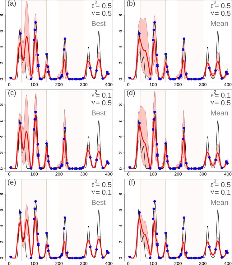
66                                                                              C. Lussana et al.: Spatial analysis of precipitation

Table 2. Overview of variables and notation for local variables. All variables are specified in the transformed space. All the vectors are
column vectors unless otherwise specified. If X is a matrix, Xi is its ith column (column vector), and Xi,: is its ith row (row vector).

                Symbol     Description                                                                    Dimension
                pi         Number of observations in the surroundings of the ith grid point               Scalar
                 i
                H          Observation operator                                                           pi × m matrix
                 i
                R          Observation error covariance matrix                                            pi × pi matrix
                     i
                0o         Observation error correlation matrix                                           pi × pi matrix
                 ib
                y          Background at observation locations                                            pi vector
                 i
                Pb         Background error covariance matrix                                             m × m matrix
                 i
                0          Localization matrix                                                            m × m matrix
                 i
                V          Localization between grid points and observation locations                     m × pi matrix
                 i
                Z          Localization between observation locations                                     pi × pi matrix
                     i
                0u         Scale correlation matrix                                                       m × m matrix
                 i
                Gb         Background error covariances between grid points and observation locations     m × pi matrix
                 i
                Sb         Background error covariances between observation locations                     pi × pi matrix
                 i
                Gf         Forecast error covariances between grid points and observation locations       m × pi matrix
                 i
                Sf         Forecast error covariances between observation locations                       pi × pi matrix
                i
                σ 2o       Observation error variance                                                     Scalar
                i
                σ 2b       Average background error variance                                              Scalar
                i                                i
                σ 2b0      Empirical estimate of σ 2b                                                     Scalar
                i
                σ 2f       Average forecast error variance                                                Scalar
                i
                σ 2u       Error variance for the scale matrix                                            Scalar
                i
                σ 2ob      Sum of error variances (Eq. 11)                                                Scalar

ensemble members reports precipitation in less than 10 % of             in the example of Sect. 3.1. In principle, the statistical inter-
the grid points; otherwise, we have wet weather. In the case            polation is sensitive to the small amount ξ chosen, such that
of wet conditions, ensemble members are considered sepa-                using 0.01 mm instead of 0.0001 mm will return slightly dif-
rately, and for each of them, we derive a single value of shape         ferent analysis values in the transition between precipitation
and a single value of rate – both are kept as constants over            and no precipitation. In practice, we have tested it, and we
the whole domain. The values of shape and rate are the maxi-            found negligible differences when values smaller than, for
mum likelihood estimators calculated iteratively by means of            example, 0.05 mm (half of the precision of a standard rain
the Newton–Raphson method as described by Wilks (2019),                 gauge measurement) have been used.
Sect. 4.6.2. Then, αD and βD are the averages of all the val-              The transformation function g(x), applied to the generic
ues of shape (one value for each ensemble member) and rate              scalar value x, used in Eqs. (1) and (2) is as follows:
(one value for each ensemble member). In the case of dry
weather, αD and βD are set to typical values obtained as the            g(x) = QNorm (Gamma(x + ξ ; αD , βD )) ,                      (3)
averages of all the available cases.
   In Gaussian anamorphosis, zero precipitation values must             where Gamma(x + ξ ; αD , βD ) is the gamma cumulative dis-
be treated as special cases, as explained by Lien et al. (2013).        tribution function when the shape is equal to αD and the rate
The solution we adopted is to first add a very small amount to          is equal to βD . QNorm is the quantile function (or inverse
zero precipitation values, ξ = 0.0001 mm, and then to apply             cumulative distribution function) for the standard Gaussian
the transformation g() to all values. The same small amount             distribution. An example of an application of the procedure
is then subtracted after the inverse transformation. This is a          described above is given in Sect. 3.2.2.
simple but effective solution for spatial analysis, as shown               For the presented implementation of EnSI-GAP, the Gaus-
                                                                        sian anamorphosis is based on the constant parameters of αD

Nonlin. Processes Geophys., 28, 61–91, 2021                                                   https://doi.org/10.5194/npg-28-61-2021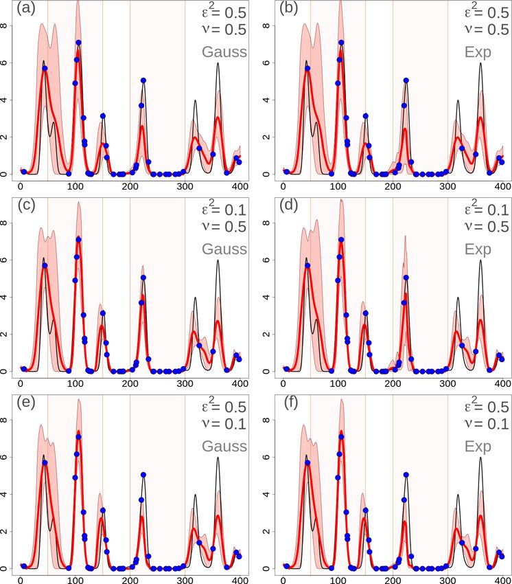
C. Lussana et al.: Spatial analysis of precipitation                                                                                 67

and βD over the whole domain. This assumption might be                  the ith grid point is a normal random variable, and our sta-
                                                                                                                                a
too restrictive for very large domains, such as for all of Eu-                                     p areturns its mean value xi and its
                                                                        tistical interpolation scheme
                                                                                               a
rope, for instance. In this case, different solutions may be            standard deviation σi = Pii .
explored, such as slowly varying the gamma parameters in                   As for linear filtering theory (Jazwinski, 2007), the anal-
space or time, based on the climatology.                                ysis is obtained as a linear combination of the background
                                                                        (a priori information) and the observations. The background
2.2     Spatial analysis                                                is written as x b = x t + ηb , where
                                                                                                          the background error is a
                                                                        random variable ηb ∼ N 0, Pb . The background PDF is de-
The spatial analysis in Algorithm 1 has been divided into               termined mostly, but not exclusively, by the forecast ensem-
three parts. In Sect. 2.2.1, global variables have been defined.        ble, as described in Sect. 2.2.1. The forecast ensemble mean
Then, as stated in the introduction of Sect. 2, the analysis            is x f = k −1 Xf 1, where 1 is the m vector, with all elements
procedure is performed on a grid point by grid point basis. In          equal to 1. The background expected value is set to the fore-
Sects. 2.2.2 and 2.2.3, the procedure applied at the generic ith        cast ensemble mean, x b = x f . The forecast perturbations are
grid point is described. In Sect. 2.2.2, the specification of the       Af , where the ith perturbation is Afi = Xfi − x f . The covari-
local error covariance matrices is described. In Sect. 2.2.3,           ance matrix is as follows:
the standard analysis procedure is presented together with the
treatment of a special case.                                            Pf = (k − 1)−1 Af (Af )T ,                                  (5)
                                                                        and plays a role in the determination of      Pb ,
                                                                                                                        as defined in
2.2.1        Definitions                                                Sect. 2.2.2.
                                                                           The p observations are written as y o = Hx t + εo , where
In Bayesian statistics, according to Savage (1972), a state is          the observation error εo ∼ N (0, R) is the observation opera-
“a description of the world, which is the object with which             tor that we consider as a linear function that maps Rm onto
we are concerned, leaving no relevant aspect undescribed”,              Rp .
and “the true state is the state that does in fact obtain”, i.e.,
the true description of the world. The mathematical notation            2.2.2   Specification of the observation and background
used is reported in Tables 1 and 2, and it is similar to that                   error covariance matrices
suggested by Ide et al. (1997). The object of our study is the
hourly precipitation field, x(), that is the hourly total precip-       Our definitions of the error covariance matrices follow from a
itation amount over a continuous surface covering a spatial             few general principles that we have formulated. For P1 (i.e.,
domain in terrain-following coordinates, r. Our state is the            general principle 1; hereinafter the same definition applies
discretization over a regular grid of this continuous field. The        for other references to P), background and observation uncer-
true state (our truth; x t ) at the ith grid point is the areal aver-   tainties are weather and location dependent. For P2, the back-
age as follows:                                                         ground is more uncertain, where either the forecast is more
      Z                                                                 uncertain or observations and forecasts disagree the most.
                                                                        For P3, observations are a more accurate estimate of the true
x ti = x (r) dr,                                                  (4)
                                                                        state than the background. We want to specify how much
        Vi                                                              more we trust the observations than the background in a sim-
                                                                        ple way, such as, for example, “we trust the observations
where Vi is a region surrounding the ith grid point. The size
                                                                        twice as much as the background”. For P4, the local obser-
of Vi determines the effective resolution of xt at the ith grid
                                                                        vation density must be used optimally to ensure a higher ef-
point. Our aim is to represent the truth with the smallest pos-
                                                                        fective resolution, as it has been defined in Sect. 2.2.1 where
sible Vi . The effective resolution of the truth will inevitably
                                                                        more observations are available. For P5, the spatial analysis
vary across the domain. In observation-void regions, the ef-
                                                                        at a particular hour does not require the explicit knowledge of
fective resolution will be the same as that of the numeri-
                                                                        observations and forecasts at any other hour. However, con-
cal model used as the background, which is approximately
                                                                        stants in the covariance matrices can be set, depending on the
o(10–100 km2 ) for high-resolution local area models (Müller
                                                                        history of deviations between observations and forecasts. P5
et al., 2017). In observation-dense regions, the effective reso-
                                                                        makes the procedure more robust and easier to implement in
lution should be comparable to the average distance between
                                                                        real-time operational applications.
observation locations, with the model resolution as the upper
                                                                           P1 and P4 led to our choice of implementing Algorithm 1
bound.
                                                                        by means of a loop over grid points. P2 will lead us to the
   The analysis is the best estimate of the truth, in the sense
                                                                        identification of the regions in which the uncertainty on the
that it is the linear, unbiased estimator with the minimum er-
                                                                        input data is greatest. P3 will be used to define the observa-
ror variance. The analysis is defined as x a = x t + ηa , where
                                                                        tional uncertainty with respect to that of the background.
the column vector of the analysis error at grid points is a
                                                                           A distinctive feature of our spatial analysis method is that
random variable following a multivariate normal distribution                                                      i
ηa ∼ N (0, Pa ). The marginal distribution of the analysis at           the background error covariance matrix Pb is specified as the

https://doi.org/10.5194/npg-28-61-2021                                                Nonlin. Processes Geophys., 28, 61–91, 2021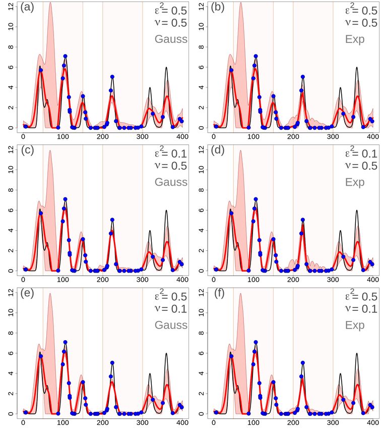
68                                                                                      C. Lussana et al.: Spatial analysis of precipitation

                                                                       i                i
sum of two parts, namely a dynamical component and a static            0 and 0 u are obtained as analytical functions of the spatial
component. This choice is consistent with P1 and P2. The                                                                      i   i
dynamical part introduces nonstationarity, while the static            coordinates. In Algorithm 1, 0 and 0 u have been specified
part describes covariance stationary random variables. This            through Gaussian functions; other possibilities for correla-
choice follows from P1, and it has been inspired by hybrid             tion functions have been described, for instance, by Gaspari
data assimilation methods (Carrassi et al., 2018). The dynam-          and Cohn (1999). We have chosen not to inflate or deflate
ical component of the background error covariance matrix is            Pf directly and to modulate the amplitude of background co-
obtained from the forecast ensemble. Because the ensemble              variances only through the terms of Eq. (6). In this way, we
has a limited size, and often the number of members is quite           reduce the number of parameters that need to be specified.
small (order of tens of members), a straightforward calcula-           As a matter of fact, for the combination of observations and
tion of the background covariance matrix will include spu-             background in the analysis procedure, the m by m covari-
rious correlations between distant points. Localization is a           ance matrices are never directly used. Instead, the matrices
technique applied in DA to fix this issue (Greybush et al.,            used are the covariances between grid points and observa-
                                                                                                    i         i       i
2011). The static component has also been introduced to
                                                                       tion locations, Gb = Pb HT (specifically only the ith row of
remedy the shortcomings of using numerical weather predic-
                                                                       this matrix is used), and the covariances between observation
tion as the background. There are deviations between obser-                                                   i
                                                                                            i       i i               i
vations and forecasts that cannot be explained by the fore-            locations Sb = HPb HT . H is the local observation operator,
cast ensemble. A typical example is when all the ensemble              which is a linear function, i.e., Rm → Rpi .
members predict no precipitation but rainfall is observed.                                                                                i
In those cases, we trust observations, as stated through P3.              The local observation error covariance matrix R is written
                                                                                                                  i
Then, the static component adds noise to the model-derived             as the constant observation error variance σ 2o multiplying the
                                                                                                          i
background error, as in the paper by Raanes et al. (2015). In          correlation matrix 0 o as follows:
Bocquet et al. (2015), the static component is referred to as
                                                                       i        i       i
a scale matrix, since it is used to scale the noise component          R = σ 2o 0 o .                                                         (7)
of the model error, and we adopt the same term here. In scale
matrix, the term scale is not associated with the concept of           i
spatial scales; instead, it refers to a scaling (amplification or      0 o is often the identity, but other choices are possible. For
reduction) of the uncertainty. We will also refer to this ma-          instance, if some observations are known to be more accu-
trix, and its related quantities, with the letter u to emphasize       rate than the average of the others, then the corresponding
                                                                                                                  i
that this component of the background error is unexplained             diagonal elements of 0 o can be set to values smaller than 1.
by the forecast.                                                       The observation uncertainty can vary in time and space, ac-
     i
     Pb is written as follows:                                         cordingly to P1; however, its spatial structure is fixed and de-
                                                                                                                                      i
i        i    i i                                                      pends on the analytical function chosen for 0 o . Note that the
Pb = 0 ◦ Pf + σ 2u 0 u .                                         (6)   observation error is not only determined by the instrumental
The first component on the right-hand side of Eq. (6) is the           error, but it also includes the representativeness error (Lus-
                                                             i         sana et al., 2010; Lorenc, 1986), which is often the largest
dynamical part. Pf is the forecast uncertainty of Eq. (5), 0 is        component of the observation error. The representative error
the localization matrix, and ◦ is the Schur product symbol.            is a consequence of the mismatch between the spatial sup-
The localization technique we apply is a combination of lo-            ports of the areal averages reconstructed by the background
cal analysis and covariance localization, as defined by Sakov          and the almost point-like observations.
and Bertino (2011). In the local analysis, only the closest               The spatial structures of the error covariance matrices are
observations are used, and we have implemented it by con-              determined through the matrices in Eqs. (6) and (7). At this
sidering only observations within a predefined spatial win-                                                   i           i
                                                                       point, we need to set σ 2u and σ 2o to scale the magnitude of the
dow surrounding each grid point, up to a preset maximum
                                                                       covariances. In the process described below, we will see that
number of pmx . The covariance localization is implemented
                                                       i
                                                                       the two variances are completely determined by two scalars,
through the element-wise multiplication of Pf by 0, which              ε 2 and ν, also defined below, that we assume to be known
has the form of a correlation matrix that depends on dis-              before running the spatial analysis. This prior knowledge de-
tances and is used to suppress long-range correlations. The            fines the constraints that the solution has to satisfy and allows
second component on the right-hand side of Eq. (6) is the              us to choose one particular solution among all the possibil-
static part. The scale matrix is expressed through a constant                       i           i
                                                                       ities. σ 2u and σ 2o characterize the region around the ith grid
                 i
variance σ 2u , which modulates the noise, and the correlation         point as a whole, without distinguishing between the individ-
             i                                                                                                                                i
matrix 0 u , which defines the spatial structure of that noise.        ual observations. We introduce two relationships linking σ 2u
                                                                            i
In the examples of applications presented in Sect. 3, both             and σ 2o through two additional variances, both expressing the

Nonlin. Processes Geophys., 28, 61–91, 2021                                                               https://doi.org/10.5194/npg-28-61-2021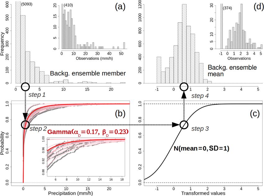
C. Lussana et al.: Spatial analysis of precipitation 69
i i
uncertainty of a quantity over the same region around the ith As a final step, to set σ 2u and σ 2o , we distinguish between
i three situations. The first situation is when the ensemble
grid point. σ 2b is the average background error variance, and
i spread is likely to underestimate the actual uncertainty be-
σ 2f is the average forecast error variance. The two relation- cause the background is missing an event or the spread is
ships are as follows: i i
too narrow. The test condition is σ 2f < σ 2b0 . We will refer to
i i this situation as the ensemble being overconfident or under-
ε 2 = σ 2o /σ 2b (8) i
dispersive. This is the case when a positive σ 2u is needed in
i i i
σ 2b = σ 2f + σ 2u . (9) i
Eq. (6), and we set its value such that σ 2b in Eq. (9) is equal
i
to σ 2b0 in Eq. (12) in the following:
ε 2 is a global variable, and it is the relative precision of the
observations with respect to the background. Equation (8)
i i i
implements P3, and ε 2 should be set to a value smaller than σ 2u = σ 2b0 − σ 2f
1. For example, ε 2 = 0.1 means that we believe the obser-
i i
i
vations to be 10 times more precise an estimate of the true = ν (y o − y b )2 /(1 + ε 2 ) − diag(Sf ) (13)
value than the background. Equation (9) is an adaptation
from Eq. (6). The next two relationships we introduce have i i i
σ 2b = ν (y o − y b )2 /(1 + ε 2 ) (14)
i
the objective of estimating σ 2f and the empirical (i.e., based
i i i
on data, not on theories) estimate of σ 2ob , which is the sum
i σ 2o = ε 2 ν (y o − y b )2 /(1 + ε 2 ). (15)
i i
of σ 2o plus σ 2b , taken directly from the forecasts and the ob-
i The second situation is when the ensemble spread is con-
served values. σ 2ob is used to obtain a reference value to judge i
if the ensemble spread is adequate. The equations are (the sistent with the empirical estimate of σ 2b . The test condition
i i i
averaging operator h. . .i is defined as in Algorithm 1) as fol- is σ 2f ≥ σ 2b0 and σ 2f > 0. We will refer to this situation as the
lows: ensemble spread being adequate. In this case, the background
information is given by the ensemble, without adjustments,
i2 i
σ f = ν diag Sf (10) and is as follows:
i
σ 2u = 0
* +
2 (16)
i i i
σ 2ob = ν yo − yb . (11)
i i i
σ 2b = σ 2f = ν diag(Sf ) (17)
ν is an inflation factor that can be used to obtain better re- i2
i
2i2 2 f
sults (e.g., via the optimization of cross-validation scores or σ o = ε σ f = ε ν diag(S ) . (18)
other verification metrics). In addition, ν is introduced be-
cause Eq. (11) is sensitive to misbehavior in the data when it Equations (13)–(18) have been written with many details,
is applied using data from one single time step. Proper esti- in a somewhat pedantic way, to emphasize the differences
i i
mates of σ 2f and σ 2ob would require more than just one case, between those two situations. When the ensemble is under-
i i
and the ideal situation would be to consider numerous situ- dispersive, the sum σ 2o + σ 2b is bounded by the upper limit
ations characterized by similar weather conditions. Instead, i
i σ 2ob . This is not the case when the ensemble is adequate.
we prefer to stick to P5. The estimation of is not resis- σ 2ob It is worth remarking that the test conditions are indepen-
tant in the sense defined by Lanzante (1996). A few outliers dent of ν. In fact, for instance, the test condition
i * for the first
2 +
in Eq. (11) may have a significant impact on σ 2ob . The intro- io ib
duction of ν makes the estimation procedure more resilient situation can be equivalently written as y −y >
in the presence of outliers and other nonstandard behavior.
i
Equation (11) is used for diagnostics in data assimilation (1 + ε 2 ) diag(Sf ) .
(Desroziers et al., 2005), and it is consistent with P2. The
The third situation is the special case in which the back-
combination of Eqs. (8) and (11) returns a rough empirical
i
ground is deemed as perfect; that is, when all the observed
estimate of σ 2b that is as follows: values and all the forecasts, at all observation locations, have
* the same value. In practice, this occurs in the case of no pre-
2 + i i
io
y −y
ib cipitation. In this case, σ 2f = 0 and σ 2b0 = 0. Errors are not
i Gaussian in this case, so then Eqs. (6) and (7) are not needed
σ 2b0 = ν . (12) anymore, as discussed in the next section (Sect. 2.2.3).
1 + ε2
https://doi.org/10.5194/npg-28-61-2021 Nonlin. Processes Geophys., 28, 61–91, 2021
70                                                                                         C. Lussana et al.: Spatial analysis of precipitation

   With reference to the working assumptions stated at the                       of synchronous realizations is considered instead of a time-
beginning of this section, they can now be reformulated in                       lagged ensemble approach. As an additional difference be-
more precise mathematical terms by referring to the above                        tween EnSI-GAP and other methods, it should be noted that
definitions and equations. P1 led us to Eqs. (6) and (7) and                     the grid point by grid point implementation makes it possi-
supported our choice of a grid point by grid point implemen-                     ble to modify the interpolation settings to adapt them to the
tation of the algorithm. P2 led us to Eq. (11) and subsequent                    different regions in the domain, as discussed in Sect. 3.1.6.
                                                     i                              The special case of a perfect background, as introduced in
equations, including the term σ 2ob . P3 led us to the introduc-
tion of ε 2 in Eq. (8). P4 is also a key reason for having an al-                Sect. 2.2.2, leads to a perfect analysis of x ai = x bi . Because
gorithm that can be optimized as a function of the grid point                    all the information available shows an exceptional level of
under consideration. Other than that, P4 has not been used                       agreement, we have chosen to set the analysis error vari-
explicitly in this section, since it will, in general, affect the                ance to zero (i.e., background is the truth), such that for those
                             i                                                   points the analysis probability distribution functions (PDFs)
specification of 0 u in Eq. (6). In this section, we do not pos-                 are Dirac’s delta functions, and this has consequences for the
                                                 i
                                                                                 inverse transformation, as discussed in Sect. 2.3.
tulate any formulation of 0 u as being preferable to another;
this depends on the application. P4 led us to the specification                  2.3    Data inverse transformation
     i
of   0uin Algorithm 1 as a location-dependent matrix through
Di , which is the length scale determining the decrease rate                     The inverse transformation g −1 of g, described in Sect. 2.1
of the background error unexplained by the forecasts. This                       and reported in Eq. (3) for a scalar value of x, is the follow-
length scale is set in both Algorithm 1 and Sect. 3 as a func-                   ing:
tion of the observational network density in the surrounding
                                                                                 g −1 (x) = QGamma (Norm(x); αD , βD ) − ξ,                  (21)
of the ith grid point. In this sense, Di is dependent on the
characteristics of precipitation as they can be observed by                      where Norm(x) is the Gaussian cumulative distribution func-
our network. This point is discussed further in Sect. 3.1.6.                     tion. QGamma (. . .; αD , βD ) is the quantile function for the
As far as we know, and as stated in the introduction, this is                    gamma distribution with shape αD and rate βD , which are
an innovative part of our interpolation scheme since most of                     obtained as described in Sect. 2.1. ξ is a constant. If x is a
the other schemes do postulate that a single analytical cor-                     vector instead of a scalar value, then we apply Eq. (21) to its
relation function or semi-variogram is valid for the whole                       components.
spatial domain considered. P5 led us to the introduction of ν                       The inverse transformation at the ith grid point is written
in Eqs. (10) and (11).                                                           as follows:
2.2.3      Analysis procedure                                                    x̃ ai = g −1 (xai ).                                        (22)
The expressions for the analysis and its error variance are di-                  However, we need to back-transform a Gaussian PDF and
rect results of the linear filter theory (Jazwinski, 2007), and                  not a scalar value. Equation (22) returns the median of the
they are derived in several books based on different formu-                      gamma distribution associated to the ith grid point. Our goal
lations (e.g., Tarantola, 2005; Kalnay, 2003; Carrassi et al.,                   is to obtain the m vectors of the gamma shape and rate,
2018). The analysis at the ith grid point is equal to the back-                  namely α a and β a , respectively. To achieve that, the inverse
                                                                  i
ground plus a weighted average of the p innovations, while                       transformation g −1 is applied to 400 quantiles of the (uni-
the analysis error variance is derived from the error covari-                    variate) Gaussian PDF defined by x̃ ai and (σ 2 )ai ; a similar
ance matrices as follows:                                                        approach is used by Erdin et al. (2012). Then, a least mean
                                                                                 square optimization procedure is used to obtain the optimal
                            i −1 i

                 i      i               i
   x ai = x bi + Gbi,: Sb + R     yo − yb               (19)                     shape and rate that better fits the back-transformed quantiles.
                                                                                 In the special case of a perfect analysis, the analysis PDF in
                                                −1            T              the original space of hourly precipitation values is a Dirac’s
               i         i           i       i           i
(σ 2 )ai   =   Pbii   − Gbi,:        S +Rb
                                                         Gbi,:        .   (20)   delta function, and the analysis is the scalar obtained as in
                                                                                 Eq. (21) when x = x ai .
Equations (19) and (20) are also typical of optimal interpo-                        Given α a and β a , it is possible to obtain the statistics
lation, and the formulation used is similar to the one adopted                   that better represent the distribution for a specific applica-
by Uboldi et al. (2008), which follows from Ide et al. (1997).                   tion (e.g., median, 99th percentile, and so on). In Sect. 3, the
It is worth remarking that the background used in Eq. (19)                       analysis value chosen is often the mean as it is the value that
is the ensemble mean, since we have assumed x b = x f in                         minimizes the spread of the variance. However, other choices
Sect. 2.2.1. The ensemble members are used to determine the                      may be more convenient, depending on the applications, as
background error covariance matrices. The method is a mod-                       discussed by Fletcher and Zupanski (2006), where, for in-
ified version of EnOI (Evensen, 2003), where an ensemble                         stance, the mode was chosen as the best estimate. In Sect. 3,

Nonlin. Processes Geophys., 28, 61–91, 2021                                                             https://doi.org/10.5194/npg-28-61-2021
C. Lussana et al.: Spatial analysis of precipitation 71
we will also consider selected quantiles of the gamma distri- spatial continuity of the truth, an anamorphosis is used to
bution to represent analysis uncertainty. link a 400-dimensional multivariate normal (MVN) vector
with the gamma distribution. The samples from the MVN
distribution, with a prescribed continuous spatial structure,
3 Results are obtained from the descriptions by Wilks (2019) in chap.
12.4. The MVN mean is a vector with 400 components all
The aim of this section is to provide guidance on the imple- set to zero, and the covariance matrix is determined using
mentation of EnSI-GAP for some applications that we con- a Gaussian covariance function with 10 u as the reference
sider important or useful for understanding how it works. length used for scaling distances. The effective resolution
In Sect. 3.1, EnSI-GAP is applied over a one-dimensional (Sect. 2.2.1) of the truth is then 10 u.
grid and in a controlled environment, using synthetic data The ensemble background (gray lines in Fig. 1a) on the
specifically generated for testing EnSI-GAP on precipitation. grid, with 10 members, is obtained by perturbing the truth.
In Sect. 3.2, a second, more realistic, example of applica- The background values at the observation locations are ob-
tion for EnSI-GAP is reported, where the spatial analysis is tained from the members using nearest-neighbor interpola-
performed for a case study of convective precipitation over tions. For each member, the truth is perturbed by shifting it
South Norway. The case study cannot be strictly considered along the grid by a random number between −10 and +10 u,
an evaluation of the method since all the available observa- thus simulating the misplacement of precipitation events.
tions are used in the spatial analysis, and it is not possible to Then, the effective resolution of the member is set to be
validate the predictions where no observations are available. coarser than that of the truth. The true values are multiplied
It is an example intended to show the potential of EnSI-GAP by coefficients derived from a uniform distribution, with val-
for (automatic) weather forecasting or civil protection pur- ues between 0.05 and 2 and a spatial structure function given
poses. by a MVN with a Gaussian covariance function, with a ref-
Section 3.3 describes the results of cross-validation ex- erence length extracted from a Gaussian distribution with a
periments over South Norway. EnSI-GAP performances are mean of 50 u and a standard deviation of 5 u. Two special
evaluated for a period of 5 months centered over summer regions are considered, and they are shown with the bright
2019, i.e., from May to September. The verification scores shading in Fig. 1. In region R1, between 50 and 150 u, each
considered are commonly used in forecast verification and background member follows an alternative truth (i.e., it is lit-
described by several books, such as, for example, Jolliffe erally being derived from a different truth) that is everywhere
and Stephenson (2012). A further useful reference for the different from 0 mm. In R1, the background is neither accu-
scores is the website of the World Meteorological Orga- rate nor precise, and this leads to the occurrence of misses
nization, available at https://www.wmo.int/pages/prog/arep/ and false alarms. In region R2, between 200 and 300 u, none
wwrp/new/jwgfvr.html (last access: 13 May 2020). of the ensemble members simulate precipitation while the
true state reports precipitation. In this region, the background
3.1 One-dimensional simulations
is precise but not accurate since the ensemble is missing, or
The aim of this section is to show how EnSI-GAP works and poorly representing, an event which is otherwise well cov-
to assess its performances with different configurations under ered by observations. Because we had to ensure the continu-
idealized conditions. The impacts of Gaussian anamorpho- ity of the background, we have enforced smooth transitions
sis and different specifications of background error covari- between the two regions and their surroundings. For exam-
ances are also investigated. The functioning of the algorithm ple, R2 is actually beginning a bit after 200 u and ending a
is shown with the example application to a single simulation. bit before 300 u.
The conclusions on the EnSI-GAP pros and cons are based The number of observations (blue dots in Fig. 1a) is set to
on the statistics collected over 100 simulations. 40. The observed value at a location is obtained as the true
value of the nearest grid point, plus a random noise that is de-
3.1.1 Simulation setup termined as a random number between −0.02 and 0.02 that
multiplies the true value. The procedure is consistent with
A one-dimensional grid with 400 points and a spacing of the fact that observation precipitation errors should follow a
1 spatial unit, or 1 u, is considered. The domain covers the multiplicative model (Tian et al., 2013). The observation lo-
region from 0.5 to 400.5 u, and the generic ith grid point cations are randomly chosen. There are five between 1 and
is placed at the coordinate i u. A simulation begins with the 100 u, 30 between 101 and 300 u, and five between the 301
creation of a true state, and then observations and ensemble and 400 u. The distribution is denser in the central part of the
background are derived from it. domain and sparser closer to the borders.
The simulation presented here is shown in Fig. 1a. For The effect of the Gaussian anamorphosis is shown in
each grid point, the true value (black line) is generated by Fig. 1b. The transformed precipitation varies within a smaller
a random extraction from the gamma distribution, with the range than the original precipitation, thus effectively short-
shape and rate set to 0.2 and 0.1, respectively. To ensure
https://doi.org/10.5194/npg-28-61-2021 Nonlin. Processes Geophys., 28, 61–91, 202172 C. Lussana et al.: Spatial analysis of precipitation
Figure 1. One-dimensional simulation. (a) Precipitation (in millimeters) – truth (black line), observations (blue dots), and background (gray
lines). (b) Transformed values. (c) Reference length scale for the scale matrix Di (units u, as defined in Sect. 3.1). Di is bounded within 3
and 20 u. (d) Integral data influence (IDI) based on Di from (c). The two regions, R1 and R2, have been highlighted with different shading
in the background of each panel.
i i
ening the tail of the distribution, reducing its skewness, and
the calculation of Pb in Eq. (6) because the part of Pb , tak-
making it more similar to a Gaussian distribution.
ing into account the atmospheric dynamics, does not depend
An example application of EnSI-GAP is presented in Al-
on the observational network. Where the IDI is close to zero,
gorithm 1. The choices that are kept fixed and that will not
the analysis is as good as the background. Figure 1d shows
vary for the whole Sect. 3.1.1 are described in this para-
i
the IDI when Di is set as the distance between the ith grid
graph. The localization matrix 0 of Eq. (6) is specified using point and its third-closest observation location. EnSI-GAP is
Gaussian functions, taking the form of those used in Algo- very sensitive to the tuning of Di , and its estimation is further
i i discussed in Sect. 3.1.6.
rithm 1 for Z and V, with Li = 25 u for all the grid points.
The sensitivity of the results to variations in the specifica-
3.1.2 Evaluation scores
tion of the scale matrix will be investigated in Sect. 3.1.3;
nonetheless, the strategy for determining Di will always be
the same whether we choose to use a Gaussian function, as The evaluation of analysis versus truth at grid points are eval-
in Algorithm 1, or an exponential function. Di is determined uated using two scores that are applied over precipitation
adaptively at each grid point, as shown in Fig. 1c, as the dis- values. The mean squared error skill score (MSESS) quan-
tance between the ith grid point and its third-closest obser- tifies the agreement between the analysis expected value and
vation location. In addition, Di has been constrained to vary the truth. The continuous ranked probability score (CRPS)
between 5 and 20 u. The tool used to quantify the impact of is a much used measure of performance for probabilistic
the spatial distribution of the observations on the analysis is forecasts. The definitions of both scores can be found, for
the integral data influence (IDI; Uboldi et al., 2008); this is a example, in Wilks (2019). The MSESS has been used for
parameter that stays close to 1 for observation-dense regions, studies on precipitation by, for example, Isotta et al. (2019),
while it is exactly equal to 0 in observation-void regions. In while applications of CRPS to precipitation can be found, for
practice, the IDI at the ith grid point is computed here as the example, in the paper by Hersbach (2000). The definitions
analysis in Eq. (19), when all the observations are set to 1 adapted to our case are reported here, in the following:
and the background is set to 0. IDI has been adapted to EnSI-
GAP in the sense that only the scale matrix is considered in 1 Pm a t 2 m
m i=1 (x̃ i − x̃ i ) 1X
MSESS = 1 − ;c = x̃ t . (23)
1 m t 2 m i=1 i
P
m i=1 (x̃ i − c)
Nonlin. Processes Geophys., 28, 61–91, 2021 https://doi.org/10.5194/npg-28-61-2021You can also read