COMPARISON OF AIRCRAFT MEASUREMENTS DURING GOAMAZON2014/5 AND ACRIDICON-CHUVA
←
→
Page content transcription
If your browser does not render page correctly, please read the page content below
Atmos. Meas. Tech., 13, 661–684, 2020
https://doi.org/10.5194/amt-13-661-2020
© Author(s) 2020. This work is distributed under
the Creative Commons Attribution 4.0 License.

Comparison of aircraft measurements during GoAmazon2014/5
and ACRIDICON-CHUVA
Fan Mei1 , Jian Wang2,16 , Jennifer M. Comstock1 , Ralf Weigel3 , Martina Krämer4,3 , Christoph Mahnke3,5 ,
John E. Shilling1 , Johannes Schneider5 , Christiane Schulz5 , Charles N. Long6 , Manfred Wendisch7 ,
Luiz A. T. Machado8 , Beat Schmid1 , Trismono Krisna7 , Mikhail Pekour1 , John Hubbe1 , Andreas Giez9 ,
Bernadett Weinzierl10 , Martin Zoeger9 , Mira L. Pöhlker5 , Hans Schlager9 , Micael A. Cecchini11 ,
Meinrat O. Andreae5,12 , Scot T. Martin13 , Suzane S. de Sá13 , Jiwen Fan1 , Jason Tomlinson1 , Stephen Springston2 ,
Ulrich Pöschl5 , Paulo Artaxo14 , Christopher Pöhlker5 , Thomas Klimach5 , Andreas Minikin15 , Armin Afchine4 , and
Stephan Borrmann3,5
1 Pacific Northwest National Laboratory, Richland, WA, USA
2 Brookhaven    National Laboratory, Upton, NY, USA
3 Institute for Physics of the Atmosphere, Johannes Gutenberg University, Mainz, Germany
4 Research Centre Jülich, Institute for Energy and Climate Research 7: Stratosphere (IEK-7), Jülich, Germany
5 Max Planck Institute for Chemistry, Mainz, Germany
6 NOAA ESRL GMD/CIRES, Boulder, CO, USA
7 University of Leipzig, Leipzig, Germany
8 National Institute for Space Research (INPE), São Paulo, Brazil
9 Deutsches Zentrum für Luft- und Raumfahrt (DLR), Oberpfaffenhofen, Germany
10 University of Vienna, Vienna, Austria
11 University of São Paulo (USP), São Paulo, Brazil
12 Scripps Institution of Oceanography, University of California San Diego, La Jolla, CA, USA
13 Harvard University, Cambridge, MA, USA
14 Instituto de Física, Universidade de São Paulo, São Paulo, Brazil
15 DLR Oberpfaffenhofen, Flight Experiments Facility, Wessling, Germany
16 Center for Aerosol Science and Engineering, Department of Energy, Environmental and Chemical Engineering,

Washington University in St. Louis, St. Louis, MO, USA

Correspondence: Fan Mei (fan.mei@pnnl.gov)

Received: 14 January 2019 – Discussion started: 29 April 2019
Revised: 23 December 2019 – Accepted: 16 January 2020 – Published: 11 February 2020

Abstract. The indirect effect of atmospheric aerosol parti-     surrounding atmospheric environment of the rainforest and
cles on the Earth’s radiation balance remains one of the most   to investigate its role in the life cycle of convective clouds.
uncertain components affecting climate change through-          During one of the intensive observation periods (IOPs) in
out the industrial period. The large uncertainty is partly      the dry season from 1 September to 10 October 2014, com-
due to the incomplete understanding of aerosol–cloud in-        prehensive measurements of trace gases and aerosol prop-
teractions. One objective of the GoAmazon2014/5 and the         erties were carried out at several ground sites. In a coordi-
ACRIDICON (Aerosol, Cloud, Precipitation, and Radiation         nated way, the advanced suites of sophisticated in situ in-
Interactions and Dynamics of Convective Cloud Systems)-         struments were deployed aboard both the US Department
CHUVA (Cloud Processes of the Main Precipitation Systems        of Energy Gulfstream-1 (G1) aircraft and the German High
in Brazil) projects was to understand the influence of emis-    Altitude and Long-Range Research Aircraft (HALO) during
sions from the tropical megacity of Manaus (Brazil) on the      three coordinated flights on 9 and 21 September and 1 Oc-

Published by Copernicus Publications on behalf of the European Geosciences Union.
662                                                                      F. Mei et al.: Comparison of aircraft measurements

tober. Here, we report on the comparison of measurements           the German High Altitude and Long Range Research Aircraft
collected by the two aircraft during these three flights. Such     (HALO). These two aircraft are among the most advanced in
comparisons are challenging but essential for assessing the        atmospheric research, deploying suites of sophisticated and
data quality from the individual platforms and quantifying         well-calibrated instruments (Schmid et al., 2014; Wendisch
their uncertainty sources. Similar instruments mounted on          et al., 2016). The pollution plume from Manaus was inten-
the G1 and HALO collected vertical profile measurements of         sively sampled during the G1 and HALO flights and also by
aerosol particle number concentrations and size distribution,      the DOE Atmospheric Radiation Measurement (ARM) pro-
cloud condensation nuclei concentrations, ozone and carbon         gram Mobile Aerosol Observing System and ARM Mobile
monoxide mixing ratios, cloud droplet size distributions, and      Facility located at one of the downwind surface sites (T3
downward solar irradiance. We find that the above measure-         site – 70 km west of Manaus). The routine ground measure-
ments from the two aircraft agreed within the measurement          ments with coordinated and intensive observations from both
uncertainties. The relative fraction of the aerosol chemical       aircraft provided an extensive data set of multi-dimensional
composition measured by instruments on HALO agreed with            observations in the region, which serves (i) to improve the
the corresponding G1 data, although the total mass loadings        scientific understanding of the influence of the emissions of
only have a good agreement at high altitudes. Furthermore,         the tropical megacity of Manaus (Brazil) on the surrounding
possible causes of the discrepancies between measurements          atmospheric environment of the rainforest and (ii) to under-
on the G1 and HALO are examined in this paper. Based on            stand the life cycle of deep convective clouds and study open
these results, criteria for meaningful aircraft measurement        questions related to their influence on the atmospheric energy
comparisons are discussed.                                         budget and hydrological cycle.
                                                                      As more and more data sets are merged to link the ground-
                                                                   based measurements with aircraft observations, and as more
                                                                   studies focus on the spatial variation and temporal evolution
1   Introduction                                                   of the atmospheric properties, it is critical to quantify the un-
                                                                   certainty ranges when combining the data collected from the
Dominated by biogenic sources, the Amazon basin is one             different platforms. Due to the challenges of airborne opera-
of the few remaining continental regions where atmospheric         tions, especially when two aircraft are involved in data col-
conditions realistically represent those of the pristine or pre-   lection in the same area, direct comparison studies are rare.
industrial era (Andreae et al., 2015). As a natural climatic       However, this type of research is critical for further com-
“chamber”, the area around the urban region of Manaus in           bining the data sets between the ground sites and aircraft.
central Amazonia is an ideal location for studying the at-         Thus, the main objectives of the study herein are to demon-
mosphere under natural conditions as well as under condi-          strate how to achieve meaningful comparisons between two
tions influenced by human activities and biomass burning           moving platforms, to conduct detailed comparisons between
events (Andreae et al., 2015; Artaxo et al., 2013; Davidson        data collected by two aircraft, to identify the potential mea-
et al., 2012; Keller et al., 2009; Kuhn et al., 2010; Martin et    surement issues, to quantify reasonable uncertainty ranges
al., 2016b; Pöhlker et al., 2018; Poschl et al., 2010; Salati      of the extensive collection of measurements, and to evalu-
and Vose, 1984). The Observations and Modeling of the              ate the measurement sensitivities to the temporal and spatial
Green Ocean Amazon (GoAmazon2014/5) campaign was                   variance. The comparisons and the related uncertainty esti-
conducted in 2014 and 2015 (Martin et al., 2016b, 2017).           mations quantify the current measurement limits, which pro-
The primary objective of GoAmazon2014/5 was to improve             vide realistic measurement ranges to climate models as initial
the quantitative understanding of the effects of anthropogenic     conditions to evaluate their output.
influences on atmospheric chemistry and aerosol–cloud in-             The combined GoAmazon2014/5 and ACRIDICON-
teractions in the tropical rainforest area. During the dry sea-    CHUVA field campaigns not only provide critical measure-
son in 2014, the ACRIDICON (Aerosol, Cloud, Precipita-             ments of aerosol and cloud properties in an undersampled
tion, and Radiation Interactions and Dynamics of Convec-           geographic region but also offer a unique opportunity to un-
tive Cloud Systems)-CHUVA (Cloud Processes of the Main             derstand and quantify the quality of these measurements us-
Precipitation Systems in Brazil) campaign also took place to       ing carefully orchestrated comparison flights. The compar-
study tropical convective clouds and precipitation over Ama-       isons between the measurements from similar instruments
zonia (Wendisch et al., 2016).                                     on the two research aircraft can be used to identify poten-
   A feature of the GoAmazon 2014/5 field campaign was             tial measurement issues and quantify the uncertainty range of
the design of the ground sites’ location, which uses princi-       the field measurements, which include primary meteorologi-
ples of Lagrangian sampling to align the sites with the Man-       cal variables (Sect. 3.1), trace gas concentrations (Sect. 3.2),
aus pollution plume (Fig. 1: source location – Manaus (T1          aerosol particle properties (number concentration, size dis-
site), and downwind location – Manacapuru (T3 site)). The          tribution, chemical composition, and microphysical proper-
ground sites were overflown with the low-altitude US De-           ties) (Sect. 3.3), cloud properties (Sect. 3.4), and downward
partment of Energy (DOE) Gulfstream-1 (G1) aircraft and            solar irradiance (Sect. 3.5). We evaluate the consistency be-

Atmos. Meas. Tech., 13, 661–684, 2020                                                  www.atmos-meas-tech.net/13/661/2020/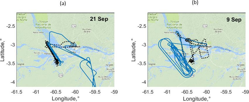
F. Mei et al.: Comparison of aircraft measurements                                                                                        663

Figure 1. Coordinated flight tracks for 21 September (a) and 9 September (b). The dotted black line is the flight track of the G1, and the blue
line is the flight track of HALO. (This figure was created using Mapping Toolbox™ © COPYRIGHT 1997–2019 by The MathWorks, Inc.)

tween the measurements aboard the two aircraft for a nearly               (Webster and Freudinger, 2018). For static temperature mea-
full set of gas, aerosol particle, and cloud variables. Results           surement, the uncertainty given by the manufacturer (Emer-
from this comparison study provide the foundation not only                son) is ±0.1 K, and the uncertainty of the field data is
for assessing and interpreting the observations from multiple             ±0.5 K. The static pressure had a measurement uncertainty
platforms (from the ground to low altitude and then to high               of 0.5 hPa. The standard measurement uncertainties were
altitude) but also for providing high-quality data to improve             ±2 K for the chilled mirror hygrometer and 0.5 ms−1 for
the understanding of the accuracy of the measurements re-                 wind speed.
lated to the effects of human activities in Manaus on local air              On HALO, primary meteorological data were obtained
quality, terrestrial ecosystems in the rainforest, and tropical           from the Basic HALO Measurement and Sensor System
weather.                                                                  (BAHAMAS) at a 1 s time resolution. The system acquired
                                                                          data from airflow and thermodynamic sensors and from the
                                                                          aircraft avionics and a high-precision inertial reference sys-
2     Measurements                                                        tem to derive the basic meteorological parameters like pres-
                                                                          sure, temperature, the 3-D wind vector, aircraft position, and
2.1     Instruments                                                       attitude. The water vapor mixing ratio and further derived
                                                                          humidity quantities were measured by the Sophisticated Hy-
The ARM Aerial Facility deployed several in situ instru-                  grometer for Atmospheric Research (SHARC) based on di-
ments on the G1 to measure atmospheric state parame-                      rect absorption measurement by a tunable diode laser (TDL)
ters, trace gas concentrations, aerosol particle properties, and          system. The absolute accuracy of the primary meteorological
cloud characteristics (Martin et al., 2016; Schmid et al.,                data was 0.5 K for air temperature, 0.3 hPa for air pressure,
2014). The instruments installed on HALO covered measure-                 0.4–0.6 ms−1 for wind, and 5 % (±1 ppm) for water vapor
ments of meteorological, chemical, microphysical, and radi-               mixing ratio. All sensors were routinely calibrated and trace-
ation parameters. Details of measurements aboard HALO are                 able to national standards (Giez et al., 2017; Krautstrunk and
discussed in the ACRIDICON-CHUVA campaign overview                        Giez, 2012).
paper (Wendisch et al., 2016). The measurements compared
between the G1 and HALO are listed in Table 1. Details on                 2.1.2   Gas phase
maintenance and calibration of the involved instrumentation
can be found in the Supplement (Tables S1 and S2).                        Constrained by data availability, the comparison of trace
                                                                          gas measurements is focused on carbon monoxide (CO) and
2.1.1    Atmospheric parameters                                           ozone (O3 ) concentrations. Those measurements were made
                                                                          aboard the G1 by a CO/N2 O/H2 O instrument (Los Gatos
All G1 and HALO meteorological sensors were routinely                     Integrated Cavity Output Spectroscopy instrument model
calibrated to maintain measurement accuracy. The G1 pri-                  907-0015-0001), and an ozone analyzer (Thermo Scientific,
mary meteorological data were provided at a 1 s time reso-                model 49i), respectively. The G1 CO analyzer was calibrated
lution based on the standard developed by the Inter-Agency                for response daily by NIST-traceable commercial standards
Working Group for Airborne Data and Telemetry Systems                     before the flight. Due to the difference between laboratory

www.atmos-meas-tech.net/13/661/2020/                                                            Atmos. Meas. Tech., 13, 661–684, 2020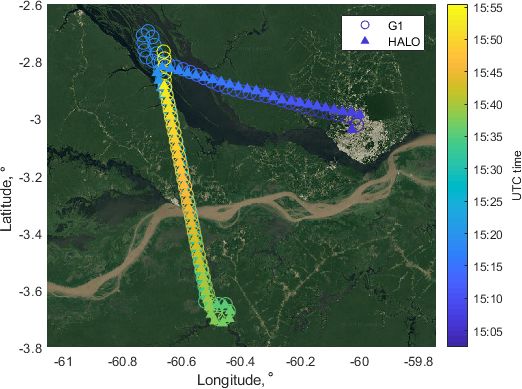
664                                                                                   F. Mei et al.: Comparison of aircraft measurements

Table 1. List of compared measurements and corresponding instruments deployed aboard the G1 and HALO during GoAmazon2014/5. The
acronyms are defined in a table at the end of this paper. Dp indicates the particle diameter. 1Dp refers to the size resolution.

        Measurement vari-                 Instruments deployed on the G1 (Martin      Instruments deployed on HALO (Wendisch et al.,
        ables                             et al., 2016; Schmid et al., 2014)          2016)
        Static pressure                   Rosemount (1201F1), 0–1400 hPa              Instrumented nose boom tray (DLR development), 0–
                                                                                      1400 hPa
        Static air temperature            Rosemount E102AL/510BF −50 to               Total air temperature (TAT) inlet
                                          +50 ◦ C                                     (Goodrich/Rosemount type 102) with an open
                                                                                      wire resistance temperature sensor (PT100), −70 to
                                                                                      +50 ◦ C
        Dew-point         tempera-        Chilled mirror hygrometer 1011B             Derived from the water vapor mixing ratio, which
        ture                              −40 to +50 ◦ C                              is measured by a tunable diode laser (TDL) system
                                                                                      (DLR development), 5–40 000 ppmv
        3-D wind                          Aircraft Integrated Meteorological Mea-     Instrumented nose boom tray (DLR development)
                                          surement System 20 (AIMMS-20)               with an air data probe (Goodrich/Rosemount) 858AJ
                                                                                      and high-precision Inertial Reference System (IGI
                                                                                      IMU-IIe)
        Particle number con-              CPC, cutoff size (Dp ) = 10 nm              CPC, cutoff size (Dp ) = 10 nm
        centration
        Size distribution∗                UHSAS-A, 60–1000 nm                         UHSAS-A, 60–1000 nm
                                          FIMS, 20–500 nm
        Non-refractory parti-             HR-ToF-AMS: organics, sulfate, nitrate,     C-ToF-AMS: organics, sulfate, nitrate, ammonium,
        cle chemical composi-             ammonium, chloride, 60–1000 nm              chloride, 60–1000 nm
        tion
        CCN concentration                 CCN-200, SS = 0.25, 0.5 %                   CCN-200, SS = 0.13 %–0.53 %
        Gas-phase concentra-              N2 O/CO and ozone analyzer, CO, O3          N2 O/CO and ozone analyzer, CO, O3 concentration,
        tion                              concentration, precision 2 ppb              precision 2 ppb
        Cloud properties*                 CDP, 2–50 µm, 1Dp = 1–2 µm                  CCP-CDP, 2.5–46 µm, 1Dp = 1–2 µm
                                          FCDP, 2–50 µm, 1Dp = 1–2 µm                 NIXE-CAS: 0.61–52.5 µm
                                          2DS, 10–1000 µm                             NIXE-CIPgs, 15–960 µm
                                                                                      CCP-CIPgs: 15–960 µm
        Radiation                         SPN1 downward irradiance, 400–              SMART-Albedometer, downward spectral irradiance,
                                          2700 nm                                     300–2200 nm
      ∗ For an individual flight, the size range may vary.

and field conditions, the uncertainty of the CO measure-                      2.1.3     Aerosol
ments is about ±5 % for 1 s sampling periods. An ultra-
fast carbon monoxide monitor (Aero Laser GmbH, AL5002)
                                                                              Aerosol number concentration was measured by different
was deployed on HALO. The detection of CO is based on
                                                                              condensation particle counters (CPCs) on the G1 (TSI, CPC
vacuum-ultraviolet fluorimetry, employing the excitation of
                                                                              3010) and HALO (Grimm, CPC model 5.410). Although two
CO at 150 nm, and the precision is 2 ppb, and the accuracy
                                                                              CPCs were from different manufacturers, they were designed
is about 5 %. The ozone analyzer measures ozone concentra-
                                                                              using the same principle, which is to detect particles by con-
tion based on the absorbance of ultraviolet light at a wave-
                                                                              densing butanol vapor on the particles to grow them to a large
length of 254 nm. The ozone analyzer (Thermo Scientific,
                                                                              enough size that they can be counted optically. Both CPCs
model 49c) in the HALO payload is very similar to the one
                                                                              were routinely calibrated in the lab and reported the data
on the G1 (model 49i), with an accuracy greater than 2 ppb or
                                                                              at a 1 s time resolution. The HALO CPC operated at 0.6–
about ±5 % for 4 s sampling periods. The G1 ozone monitor
                                                                              1 L min−1 , with a nominal cutoff of 4 nm. Due to inlet losses,
was calibrated at the New York State Department of Environ-
                                                                              the effective cutoff diameter increases to 9.2 nm at 1000 hPa,
mental Conservation testing laboratory in Albany.
                                                                              and 11.2 nm at 500 hPa (Andreae et al., 2018; Petzold et al.,

Atmos. Meas. Tech., 13, 661–684, 2020                                                               www.atmos-meas-tech.net/13/661/2020/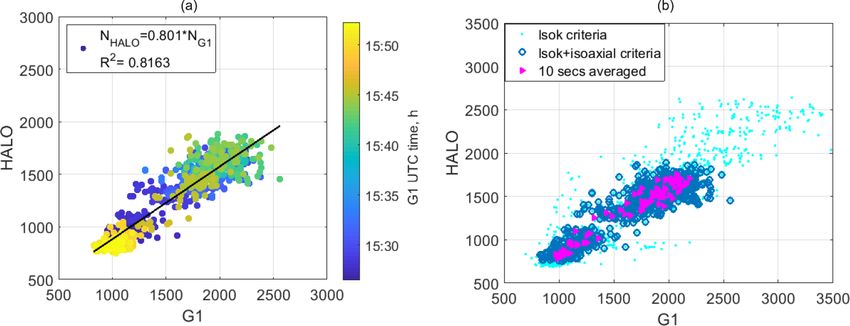
F. Mei et al.: Comparison of aircraft measurements                                                                            665

2011). The G1 CPC operated at 1 L min−1 volumetric flow            (3σ values) µg m−3 for organic, sulfate, nitrate, and ammo-
rate and the nominal cutoff diameter D50 measured in the lab       nium, respectively (DeCarlo et al., 2006). A compact time-
was ∼ 10 nm. During a flight, the cutoff diameter may vary         of-flight aerosol mass spectrometer (C-ToF-AMS) was op-
due to tubing losses, which contributes less than 10 % uncer-      erated aboard HALO to investigate the aerosol composition.
tainty to the comparison between two CPC concentrations.           Aerosol particles enter both the C-ToF-AMS and HR-ToF-
   Two instruments deployed on the G1 measured aerosol             AMS via constant pressure inlets controlling the volumetric
particle size distribution: a Fast Integrated Mobility Spec-       flow into the instrument, although the designs of the inlets
trometer (FIMS) inside the G1 cabin measured the aerosol           are somewhat different (Bahreini et al., 2008). The details
mobility size from 15 to 400 nm (Kulkarni and Wang, 2006a,         about the C-ToF-AMS operation and data analysis are re-
b; Olfert et al., 2008; Wang, 2009). The ambient aerosol par-      ported Schulz et al. (2018). The overall accuracy has been
ticles were charged after entering the FIMS inlet and then         reported as ∼ 30 % for both AMS instruments (Alfarra et
separated into different trajectories in an electric field based   al., 2004; Middlebrook et al., 2012). Data presented in this
on their electrical mobility. The spatially separated particles    section were converted to the same conditions as the HALO
grow into supermicrometer droplets in a condenser where su-        AMS data, which are 995 hPa and 300 K. Both AMS instru-
persaturation of the working fluid is generated by cooling. At     ments were calibrated before and after the field deployment
the exit of the condenser, a high-speed charge-coupled device      and also once a week during the field campaign.
camera captures the image of an illuminated grown droplet             The number concentration of cloud condensation nuclei
at high resolution. In this study, we used the FIMS 1 Hz data      (CCN) was measured aboard both aircraft using the same
for comparison. The size distribution data from FIMS were          type of CCN counter from Droplet Measurement Technolo-
smoothed. Aside from the FIMS, the airborne version of the         gies (DMT, model 200). This CCN counter contains two
Ultra High Sensitivity Aerosol Spectrometer (UHSAS) was            continuous-flow, thermal-gradient diffusion chambers for
deployed on G1 and HALO. The G1 and HALO UHSASs                    measuring aerosols that can be activated at constant supersat-
were manufactured by the same company, and both were               uration. The supersaturation is created by taking advantage
mounted under the wing on a pylon. UHSAS is an optical-            of the different diffusion rates between water vapor and heat.
scattering, laser-based particle spectrometer system. The size     After the supersaturated water vapor condenses on the CCN
resolution is around 5 % of the particle size. The G1 UHSAS        in the sample air, droplets are formed, counted, and sized by
typically covered a size range of 60 to 1000 nm. HALO UH-          an optical particle counter (OPC). The sampling frequency
SAS covered a 90 to 500 nm size range for the 9 September          is 1 s for both deployed CCN counters. Both CCN counters
flight.                                                            were calibrated using ammonium sulfate aerosol particles in
   Based on operating principles, FIMS measures aerosol            the diameter range of 20–200 nm. The uncertainty of the ef-
electrical mobility size, and UHSAS measures the aerosol           fective water vapor supersaturation was ±5 %. (Rose et al.,
optical equivalent size. Thus, the difference in the averaged      2008)
size distributions from those two types of instruments might
be linked to differences in their underlying operating prin-       2.1.4   Clouds
ciples, such as the assumption in the optical properties of
aerosol particles. The data processing in the G1 UHSAS             Aircraft-based measurements are an essential method for in
assumed that the particle refractive index is similar to am-       situ samplings of cloud properties (Brenguier et al., 2013;
monium sulfate (1.55), which is larger than the average re-        Wendisch and Brenguier, 2013). Over the last 50–60 years,
fractive index (1.41–0.013i) from a previous Amazon study          hot-wire probes have been the most commonly used devices
(Guyon et al., 2003). The HALO UHSAS was calibrated with           to estimate liquid water content (LWC) in the cloud from re-
polystyrene latex spheres, which have a refractive index of        search aircraft. Since the 1970s, the most widely used tech-
about 1.572 for the UHSAS wavelength of 1054 nm. The un-           nique for cloud droplet spectra measurements has been de-
certainty due to the refraction index can lead to up to 10 %       veloped based on the light-scattering effect. This type of in-
variation in UHSAS measured size (Kupc et al., 2018). Also,        strument provides the cloud droplet size distribution as the
the assumption of spherical particles affects the accuracy of      primary measurement. By integrating the cloud droplet size
UHSAS sizing of ambient aerosols.                                  distribution, additional information such as LWC can be de-
   The chemical composition of submicron non-refractory            rived from the high-order data product.
(NR-PM1 ) organic and inorganic (sulfate, nitrate, ammo-              Three cloud probes from the G1 are discussed in this
nium) aerosol particles was measured using a high-resolution       paper. The cloud droplet probe (CDP) is a compact,
time-of-flight aerosol mass spectrometer (HR-ToF-AMS)              lightweight, forward-scattering cloud particle spectrometer
aboard the G1 (DeCarlo et al., 2006; Jayne et al., 2000;           that measures cloud droplets in the 2 to 50 µm size range
Shilling et al., 2013, 2018). Based on the standard devia-         (Faber et al., 2018). Using state-of-the-art electro-optics and
tion of observed aerosol mass loadings during filter mea-          electronics, Stratton Park Engineering (SPEC Inc.) devel-
surements, the HR-ToF-AMS detection limits for the aver-           oped a fast cloud droplet probe (FCDP), which also uses for-
age time of 13 s are approximately 0.13, 0.01, 0.02, and 0.01      ward scattering to determine cloud droplet distributions and

www.atmos-meas-tech.net/13/661/2020/                                                   Atmos. Meas. Tech., 13, 661–684, 2020
666                                                                       F. Mei et al.: Comparison of aircraft measurements

concentrations in the same range as CDP with up to 100 Hz         rected to gain ambient conditions using a thermodynamic ap-
sampling rate. The G1 also carried a two-dimensional stereo       proach developed by Weigel et al. (2016). For NIXE-CAPS,
probe (2DS, SPEC Inc.), which has two 128-photodiode lin-         the size distributions were provided where NIXE-CAS was
ear arrays working independently. The 2DS electronics pro-        merged with the NIXE-CIPgs at 20 µm.
duce shadowgraph images with 10 µm pixel resolution. Two
orthogonal laser beams cross in the middle of the sample          2.1.5    Solar radiation
volume, with the sample cross section for each optical path
of 0.8 cm2 . The manufacturer claims the maximum detec-           The G1 radiation suite included shortwave (SW, 400–
tion size is up to 3000 µm for the 2DS. However, due to           2700 nm) broadband total upward and downward irradiance
the counting statistic issue, the data used in this study are     measurements using Delta-T Devices model SPN1 radiome-
from 10 to 1000 µm only (Lawson et al., 2006). 2DS was            ters. The radiation data were corrected for aircraft tilt from
upgraded with modified probe tips, and an arrival time algo-      the horizontal reference plane. A methodology has been de-
rithm was applied to the 2DS data processing. Both efforts        veloped (Long et al., 2010) for using measurements of total
effectively reduced the number of small shattered particles       and diffuse shortwave irradiance and corresponding aircraft
(Lawson, 2011). For G1 cloud probes, the laboratory calibra-      navigation data (latitude, longitude, pitch, roll, heading) to
tions of the sample area and droplet sizing were performed        calculate and apply a correction for platform tilt to the broad-
before the field deployment. During the deployment, weekly        band hemispheric downward SW measurements. Addition-
calibrations with glass beads were performed with the size        ally, whatever angular offset there may be between the actual
variation of less than 5 %, which were consistent with the        orientation of each radiometer’s detector and what the navi-
pre-campaign and post-campaign calibrations. Comparison           gation data say is level has also been determined for the most
between the LWC derived from cloud droplet spectra with           accurate tilt correction.
hot-wire LWC measurement was made to estimate/eliminate              The Spectral Modular Airborne Radiation measure-
the coincidence errors in cloud droplet concentration mea-        ment sysTem (SMART-Albedometer) was installed aboard
surements (Lance et al., 2010; Wendisch et al., 1996).            HALO. Depending on the scientific objective and the con-
   Aboard HALO, two cloud probes were operated and dis-           figuration, the optical inlets determining the measured radia-
cussed in this paper, each consisting of a combination of         tive quantities can be chosen. The SMART-Albedometer has
two instruments: cloud combination probe (CCP) and a cloud        been utilized to measure the spectral upward and downward
aerosol precipitation spectrometer (CAPS, denoted as NIXE-        irradiances; thereby, it is called an albedometer, as well as
CAPS; NIXE: Novel Ice Experiment). The CCP is a com-              used to measure the spectral upward radiance. The SMART-
bination of a CDP (denoted as CCP-CDP) with a CIPgs               Albedometer is designed initially to cover measurements in
(cloud imaging probe with greyscale, DMT, denoted as CCP-         the solar spectral range between 300 and 2200 nm (Krisna
CIPgs). NIXE-CAPS consists of a CAS-Dpol (cloud and               et al., 2018; Wendisch et al., 2001., 2016). However, due to
aerosol spectrometer, DMT, denoted as NIXE-CAS) and a             the decreasing sensitivity of the spectrometer at large wave-
CIPgs (denoted as NIXE-CIPgs). CIPgs is an optical array          lengths, the use of the wavelengths was restricted to 300–
probe comparable to the 2DS operated on the G1. CIPgs ob-         1800 nm. The spectral resolution is defined by the full width
tains images of cloud elements using a 64-element photo-          at half maximum (FWHM), which is between 2 and 10 nm. In
diode array (15 µm resolution) to generate two-dimensional        this case, the instruments were mounted on an active horizon-
images with a nominal detection diameter size range from 15       tal stabilization system for keeping the horizontal position of
to 960 µm (Klingebiel et al., 2015; Molleker et al., 2014). The   the optical inlets during aircraft movements (up to ±6◦ from
CCP-CDP detects the forward-scattered laser light by cloud        the horizontal plane).
particles in the size range of 2.5 to 46 µm. The sample area of
the CCP-CDP was determined to be 0.27 ± 0.025 mm2 with            2.2     Flight patterns
an uncertainty of less than 10 % (Klingebiel et al., 2015).
CAS-Dpol (or NIXE-CAS) is a light-scattering probe com-           During the dry season IOP (1 September–10 October 2014),
parable to the CDP but covers the size range of 0.6 to 50 µm      two types of coordinated flights were carried out: one flight in
in diameter, thus including the upper size range of the aerosol   the cloud-free condition (9 September) and two flights with
particle size spectrum (Luebke et al., 2016). Furthermore,        clouds present (21 September and 1 October). In this study,
CAS-Dpol measures the polarization state of the particles         we compare the measurements for both coordinated flight
(Costa et al., 2017). Similar to the G1 CDP, the performance      patterns. The discussion is mainly focused on the flights un-
of the CCP-CDP and NIXE-CAS was frequently examined               der cloud-free conditions on 9 September and the flight with
by glass bead calibrations. Prior to or after each HALO           clouds present on 21 September, as shown in Fig. 1. The
flight, CCP-CIPgs and NIXE-CIPgs calibrations were per-           other coordinated flight on 1 October is included in the Sup-
formed by using a mainly transparent spinning disk that car-      plement (Sect. S1, Figs. S1, S2, S7, and S8).
ries opaque spots of different but known sizes. The data of the      For the cloud-free coordinated flight on 9 September, the
CCP measured particle concentration aboard HALO are cor-          G1 took off first and orbited around an area from the planned

Atmos. Meas. Tech., 13, 661–684, 2020                                                 www.atmos-meas-tech.net/13/661/2020/
F. Mei et al.: Comparison of aircraft measurements                                                                                667

Figure 2. Time-colored flight track of the G1 (circle) and HALO
(triangle) on 9 September during a cloud-free coordinated flight at
500 m a.s.l. (50 m apart as the closest distance). (This figure was
created using Mapping Toolbox™ © COPYRIGHT 1997–2019 by
The MathWorks, Inc.)                                                  Figure 3. Time-colored flight profile of the G1 (a) and HALO (b)
                                                                      on 21 September, during a coordinated flight.

rendezvous point until HALO arrived in sight. It then coordi-         length and instrument flow had been corrected. For the coor-
nated with HALO and performed a wing-to-wing maneuver                 dinated flight on 9 September, the data compared were from
along straight legs around 500 m above sea level, as shown in         the same type of measurements with the same sampling rate.
Fig. 2. The normal G1 average sampling speed is 100 m s−1 ,           For the measurements with the different sampling rate, the
and the normal HALO average sampling speed is 200 m s−1 .             data were binned to the same time interval for comparison.
During the coordinated flight on 9 September, both aircraft           For the flight with the cloud present (21 September and 1 Oc-
also adjusted their normal sampling speed by about 50 m s−1           tober), the following criteria are used: (1) the data collected
so that they could fly side by side.                                  by the two aircraft must be less than 30 min apart from each
   For the second type of coordinated flights, the G1 and             other; (2) the comparison data were binned to 200 m altitude
HALO flew the stacked pattern at their own typical airspeed.          intervals; (3) the cloud flag was applied to the aerosol mea-
On 21 September, the G1 also took off from the airport first,         surements, and the data affected by the cloud shattering are
followed by HALO 15 min later. Then, both aircraft flew               eliminated from the comparisons of aerosol measurements.
above the T3 ground site and subsequently flew several flight         Moreover, additional comparison criteria are specified for
legs stacked at different altitudes. The two aircraft were ver-       individual measurements in the following section. Table 2
tically separated by about 330 m and sampled below, inside,           shows the total number of points used for the comparison.
and above clouds. Due to the different aircraft speeds, the
time difference between two aircraft visiting the same part
of the flight paths varied, increasing up to 1 h at the end of        3     Results
the flight path, as shown in Fig. 3. On 1 October, the G1
focused on the cloud microphysical properties and contrast-           3.1    Comparison of the G1 and HALO measurements
ing polluted versus clean clouds. HALO devoted the flight                    of atmospheric state parameters
to the cloud vertical evolution and life cycle and also probed
the cloud processing of aerosol particles and trace gases. The        The atmospheric state parameters comprise the primary vari-
G1 and HALO coordinated two flight legs between 950 and               ables observed by the research aircraft. The measurements
1250 m above the T3 site under cloud-free conditions. Fol-            provide essential meteorological information not only for un-
lowing that, HALO flew to the south of Amazonia, and the              derstanding the atmospheric conditions but also for provid-
G1 continued sampling plume-influenced clouds above the               ing the sampling conditions for other measurements, such as
T3 site and then flew above the Rio Negro area.                       those of aerosol particles, trace gases, and cloud microphys-
   In this study, to perform a meaningful comparison of in            ical properties.
situ measurements, all the data from instruments were time               For cloud-free coordinated flights, the comparison focused
synchronized with the aircraft (G1 or HALO) navigation sys-           on the nearly side-by-side flight leg at around 500 m, as
tem. For AMS and CPC data, the time shifting due to tubing            shown in Fig. 2. Table 3 shows the basic statistics of the

www.atmos-meas-tech.net/13/661/2020/                                                      Atmos. Meas. Tech., 13, 661–684, 2020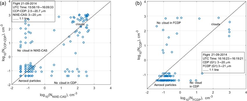
668                                                                                  F. Mei et al.: Comparison of aircraft measurements

Table 2. Summary of the total data points compared between the G1 and HALO instruments. NA – not available.

                                                                9 September 2014         21 September 2014
                                                                 G1         HALO               G1          HALO
                              Atmospheric parameters            2815         2815            7326           12065
                              Gas phase, CO                      NA           NA             7326           12065
                              Gas phase, ozone                  2815         2815            7110           11766
                              CPC                               2043         2043            8466           11646
                              UHSAS (FIMS)                      2031         2031     5841 (9405)              828
                              AMS                                NA           NA              587              818
                              CCNc                               663          531            7982             4546
                              G1: CDP(FCDP)                      NA           NA      3627 (4439)      2051 (2260)
                              HALO: CCP-CDP
                              (NIXE-CAS)
                              G1: 2DS                            NA            NA             2280     2261 (2260)
                              HALO: CCP-CIPgs
                              (NIXE-CIPgs)
                              RAD                               1355         1355              NA             NA

Table 3. Summary of basic statistics of data between in situ measurements on 9 September.

             Comparison of the coordinated flight on 9 September
                                                 G1                                      HALO
             Variables          Min       Max          Mean            SD    Min       Max      Mean        SD        Slope      R2
             T, K              297.7     300.2         298.9         0.5    297.2     299.4     298.4       0.4       1.002     Neg.
             P , hPa             955       965         960.1         1.5      958     964.9     961.8       0.9       0.998     Neg.
             WSpd, m s−1          0.3      8.9            3.4       1.2        0.3      7.7       3.8       1.1       0.998     Neg.
             Tdew , K            293     296.5         295.0        0.5     292.9     294.9     294.0       0.3       0.996     Neg.
             O3 , ppb           10.5      58.8           22.2       9.3      18.3      50.8      26.3       6.6       1.082   0.9401
             CPC, cm−3         696.0    3480.6        1591.3      568.7     687.4    2639.4    1313.8     473.5       0.819   0.8508
             UHSAS, cm−3        78.2     1118.         645.5      116.3     504.1    1622.2     756.3     138.6       1.165   0.8193
             CCNc (κ)          0.010     0.347        0.1855      0.067     0.012     0.394    0.1890     0.083      0.8937     Neg.

data for primary atmospheric state parameters, assuming that                  average dew-point temperatures was about 1 K. For temper-
two measurements from the G1 and HALO have a propor-                          ature and humidity, the G1 data were slightly higher than
tional relationship without any offset (Y = m0 × X). In gen-                  the HALO data. The main contributions to the observed
eral, the atmospheric state parameters observed from both                     differences include the error propagation in the derivation
aircraft were in excellent agreement. The linear regression                   of the ambient temperature from the measured temperature,
achieved a slope that was near 1 for four individual measure-                 instrumental-measurement uncertainty, and the temporal and
ments. The regression is evaluated using the equation below:                  spatial variability. The average horizontal wind speed mea-
                                                                              sured by HALO is 0.4 m s−1 higher than the average horizon-
           SSregression                                                       tal wind speed measured by the G1. The uncertainty source
R2 = 1 −                ,                                           (1)
            SSTotal                                                           of wind estimation is mainly due to the error propagation
                                                                              from the indicated aircraft speed measurement and the air-
where the sum  P squared regression error is calculated by                    craft ground speed estimation from GPS. The static pressure
SSregression = (yi − yregression )2P, and the sum squared total               distribution measured aboard HALO showed a smaller stan-
error is calculated by SSTotal = (yi − y)2 , yi is the indi-                  dard deviation (0.9 hPa) compared to the value of the G1
vidual data point, y is the mean value, and yregression is the                (1.5 hPa). Part of the reason for this difference is a more sub-
regression value. When the majority of the data points are in                 stantial variation of the G1 altitude during level flight legs
a narrow value range, using the mean is better than the re-                   when the G1 flew at around 50 m s−1 faster than its normal
gression line, and the R 2 will be negative (“neg.” in Table 3).              airspeed. Thus, any biases caused by their nearly side-by-side
   The difference between the average ambient temperatures
on the two aircraft was 0.5 K, and the difference between the

Atmos. Meas. Tech., 13, 661–684, 2020                                                                www.atmos-meas-tech.net/13/661/2020/
F. Mei et al.: Comparison of aircraft measurements 669
airspeeds being different from their typical airspeeds would speed (Fig. 4d) were also more significant compared to the
be undetected during these coordinated flights. variances of temperature and pressure measurements.
For the coordinated flights under cloudy conditions, we
used the criteria from Sect. 2 to compare ambient conditions 3.2 Comparison of trace gas measurements
measured by the G1 and HALO aircraft. In addition to the
ordinary linear regression, we also used the orthogonal re- For the cloud-free coordinated flight on 9 September, ozone
gression to minimize the perpendicular distances from the is the only trace gas measurement available on both aircraft.
data points to the fitted line. The ordinary linear regression The linear regression slope shows that the HALO ozone con-
assumes only the response (Y ) variable contains measure- centration was about 8 % higher than the G1 concentration.
ment error but not the predictor (X), which remains unknown The difference between the averaged ozone concentrations
when we start the comparison between the measurements was 4.1 ppb. As mentioned in Sect. 2.1.2, each instrument
from the G1 and HALO. Thus, the additional orthogonal re- has a 2 ppb accuracy (or 5 %) on the ground based on a di-
gression examines the assumption in the least squares regres- rect photometric measurement measuring the ratio between a
sion and makes sure the roles of the variables have little influ- sample and an ozone-free cell. The in-flight calibration sug-
ence on the results. In Table 4, two equations were used for gested that the accuracy of each instrument could rise to 5 %–
the orthogonal regression. One assumes that two measure- 7 % (or 2–3.5 ppb). Thus, the difference between the aver-
ments have a proportional relationship (Y = m1 × X). The aged ozone concentrations (4.1 ppb) is within the instrument
other one assumes a linear relationship, which can be de- variation. The primary source of bias is probably the different
scribed with the slope–intercept equation Y = m×X+b. The ozone loss in the sampling and transfer lines.
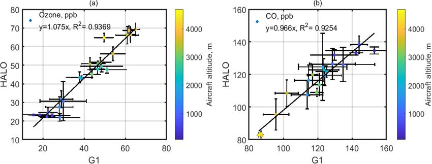
two regression results in Table 4 do not show a significant The comparison made on the 21 September flight in Fig. 5
difference. The regression using the slope–intercept equation shows good agreement for the vertically averaged ozone
shows a different level of improvement in each individual measurements. Comparing the statistics data from 9 Septem-
measurement and will be discussed in the corresponding sec- ber, the ozone measurement is not sensitive to the temporal
tions. and spatial changes. Although we do not have the compar-
As shown in Fig. 4, the linear regression slopes for ambi- ison data on 9 September, the G1 and HALO CO measure-
ent temperature (Fig. 4a), pressure (Fig. 4b), and dew-point ment comparison shows a higher correlation than the ozone
temperature were also close to 1 between the G1 and HALO data comparison at different altitudes on 21 September. Note
measurements during the 21 September coordinated flight. that the data points with more substantial variance in CO con-
The R 2 value is also close to 1. These results suggest that centration were excluded because the G1 and HALO were
the G1 and HALO measurements achieved excellent agree- sampling different air masses between 2000 and 3000 m, as
ment. Note that the dew-point temperature from the G1 mea- indicated in Figs. S3–S5. The CO plot in Fig. 5b shows the
surement was erroneous and removed from the comparison real atmospheric variability. Around 4000 m, the CO reading
the data points between 2200 and 2700 m and above 3700 m from the G1 and HALO has the minimum variation and is
(Fig. 4c) because the G1 sensor was skewed by wetting in averaged around 85 ppb, which is at the atmospheric back-
the cloud. The HALO dew-point temperature was calculated ground level. At lower altitudes and higher CO concentra-
from the total water mixing ratio measured by TDL, and that tions, the local contribution is not well mixed, and the in-
measurement in the cloud was more accurate than the mea- homogeneity is expressed as the more substantial variations
surement made by the chilled mirror hygrometer aboard the observed in the plot.
G1.
The lower value of the R 2 value in horizontal wind speed 3.3 Comparison of aerosol measurements
means the ratio of the regression error and total error in wind
measurement is much higher than the temperature and pres- Aerosol particles exhibited substantial spatial variations,
sure measurements. The main contributions to this differ- both vertically and horizontally, due to many aerosol sources
ence are the error propagation during the horizontal wind and complex atmospheric processes in the Amazon basin,
speed estimation and the temporal and spatial variance be- especially with the local anthropogenic sources in Manaus.
tween two aircraft sampling locations. We observed dif- Thus, spatially resolved measurements are critical to charac-
ferences between the two aircraft data of up to 2 m s−1 , terizing the properties of the Amazonian aerosols. The cloud-
caused by the increasing sampling distance as the two air- free coordinated flights allow us to compare the G1 and
craft were climbing up. For example, the G1 flew a level HALO aerosol measurements and thus will facilitate further
leg above T3 around 2500 m between 16:20 and 16:30 UTC, studies that utilize the airborne measurements. The vertical
while HALO stayed around 2500 m for a short period and profiles obtained using the G1 and HALO in different aerosol
kept climbing to a higher altitude. Due to strong vertical regimes of the Amazon basin have contributed to many stud-
motion, turbulence, and different saturations (evaporation– ies (Fan et al., 2018; Martin et al., 2017; Wang et al., 2016).
condensation processes), the variances in the horizontal wind The design and performance of the aircraft inlets can
strongly influence measured aerosol particle number con-
www.atmos-meas-tech.net/13/661/2020/ Atmos. Meas. Tech., 13, 661–684, 2020670 F. Mei et al.: Comparison of aircraft measurements
Table 4. Summary of three statistics analysis of data between in situ measurements on 21 September.
Comparison of the coordinated flight on 21 September
m Offset R2 m0 R2 m1 R2
T, K 0.929 20.0 0.9992 0.999 0.9928 0.999 0.9928
P , hPa 1.001 0.929 0.9998 1.001 0.9998 1.001 0.9998
WSpd, m s−1 0.885 1.0 0.7875 1.012 0.5076 1.023 0.5049
Tdew , K 0.989 3.8 0.9963 1.003 0.9904 1.003 0.9904
O3 , ppb 1.134 −1.5 0.9598 1.075 0.9369 1.101 0.9208
CO, ppb 0.922 5.4 0.9654 0.966 0.9254 0.967 0.9254
CPC, cm−3 0.571 199.4 0.9482 0.635 0.8738 0.641 0.8735
UHSAS, cm−3 1.126 178.0 0.8249 1.293 0.5070 1.384 0.4847
CCNc (κ) 0.766 55.3 0.8330 0.815 0.6544 0.829 0.6521
Figure 4. Aircraft altitude-colored plots of (a) ambient temperature, (b) static pressure, (c) dew-point temperature, and (d) horizontal wind
speed observed by the G1 and HALO on 21 September.
centration, size distribution, and chemical composition transmission efficiency larger than 90 % at 1 µm (Andreae et
(Wendisch et al., 2004). Therefore, they need to be taken into al., 2018; Minikin et al., 2017).
consideration when comparing the measurements aboard two
aircraft. The G1 aerosol inlet is a fully automated isokinetic 3.3.1 Aerosol particle number concentration
inlet. Manufacturer wind tunnel tests and earlier studies show
that this inlet operates for aerosol particles with a diameter up For the cloud-free coordinated flight on 9 September, the
to 5 µm, with transmission efficiency around 50 % at 1.5 µm linear regression of CPC and UHSAS between the G1 and
(Dolgos and Martins, 2014; Kleinman et al., 2007; Zaveri et HALO measurements is also included in Table 3. The total
al., 2010). The HALO submicrometer aerosol inlet (HASI) number concentration measured by HALO CPC was about
was explicitly designed for HALO. Based on the numerical 20 % lower than that by the G1 CPC, as shown in Fig. 6a.
flow modeling, optical particle counter measurements, and The CPC measurement is critically influenced by the isoki-
field study evaluation, HASI has a cutoff size of 3 µm, with netic inlet operation and performance. During the flights, the
Atmos. Meas. Tech., 13, 661–684, 2020 www.atmos-meas-tech.net/13/661/2020/F. Mei et al.: Comparison of aircraft measurements 671 Figure 5. Aircraft altitude-colored plots of trace gas (a) ozone and (b) CO for the coordinated flight on 21 September. Figure 6. The G1 and HALO comparison for aerosol number concentration (cm−3 ) measured by CPC (> 10 nm) on 9 September: (a) with isokinetic inlet constrain; (b) with different criteria. aircraft attitude, such as the pitch and roll angles, will cause such as systematic instrument drifts, different aerosol particle the isokinetic sampling under non-axial conditions. The non- losses inside the two CPCs, and different inlet transmission axial flow at the probe inlet may result in flow separation, efficiencies in the two aircraft. turbulence, and particle deposition. Therefore, quantitative The CPC data in Fig. 6 are color coded with UTC time. particle measurements have more substantial uncertainty. As The general trend is that the aerosol number concentration in- shown in Fig. 6b, we compared the CPC data by applying creased with time through the Manaus plume between 15:30 three different data quality criteria. The first criterion is the and 15:40 UTC. A similar trend was observed in aerosol par- same criterion described in the previous section that makes ticle number concentration (Fig. 7) measured by the UHSAS- sure all the compared measurements happen less than 30 min Airborne version (referred to as UHSAS). The total num- apart, and the linear regression is included in Table 3. The ber concentration data given by UHSAS (Fig. 7) are inte- second criterion constrains the data under the isokinetic and grated over the overlapping size range (90–500 nm for the isoaxial condition, and the plot in Fig. 6b shows the isoax- 9 September flight) for both the G1 and HALO UHSAS. The ial criteria reduced the broadness of the scattered data but no linear regression shows that the total aerosol particle number significant change to the linear regression. We further con- concentration from HALO UHSAS is about 16.5 % higher strained the data with the averaging. Based on the average than that from the G1 UHSAS. The discrepancy between wind speed and distance between two aircraft, we averaged the two UHSAS measurements is mainly due to the error the data into 10 s intervals and found that the regression R 2 propagation in the sampling flow, the differential pressure increases to 0.9392. The typical uncertainty between two transducer reading, the instrument stability, and calibration CPCs is 5 %–10 % in a well-controlled environment (Gun- repeatability, consistent with the other UHSAS study (Kupc the et al., 2009; Liu and Pui, 1974). Although both CPCs et al., 2018). In the airborne version of UHSAS, mechani- from the G1 and HALO were characterized in the lab to be cal vibrations have a more significant impact on the pressure within 10 % of their respective lab standards, we observed a transducer reading than the case for the bench version of UH- 20 % variance during the flight. This result suggests the chal- SAS. lenging condition of airborne measurement can significantly For the coordinated flight on 21 September, the G1 and increase the systematic uncertainties of CPC measurements, HALO data are averaged to 200 m vertical altitude intervals www.atmos-meas-tech.net/13/661/2020/ Atmos. Meas. Tech., 13, 661–684, 2020
672 F. Mei et al.: Comparison of aircraft measurements
agreement with HALO UHSAS and was about 30 %–50 %
higher than the G1 UHSAS depending on the particle size.
Because the UHSAS has a simplified “passive” inlet, the
large size aerosol particle loss in the UHSAS inlet was ex-
pected to increase with increasing aircraft speed. Thus, the
lower G1 UHSAS concentrations at a larger aerosol particle
size are likely related to the particle loss correction.
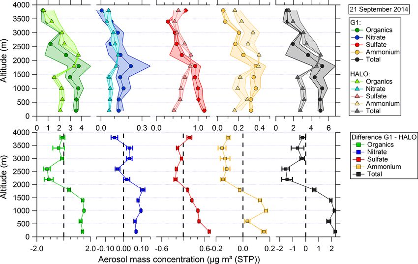
For the 21 September flight, the vertical profiles of aerosol
size distributions are averaged into 100 m altitude intervals
(Fig. 10). Overall, all size distribution measurements cap-
tured the mode near 100 nm between 800 and 1000 m at the
top of the convective boundary layer, as indicated by the
Figure 7. The G1 and HALO comparison for aerosol number con- potential temperature (Fig. 10d), which starts from a maxi-
centration measured by UHSAS (90–500 nm) on 9 September. mum near the ground and then becomes remarkably uniform
across the convective boundary layer. The peak of the aerosol
size distribution shifted from 100 to 150 nm with increasing
(Fig. 8). The data points with an altitude between 2000 and altitude. Note that due to data availability, the aerosol size
3000 m were excluded from the comparisons, because the G1 distribution data from the HALO UHSAS have a reduced
and HALO sampled different air masses, as evidenced from vertical resolution.
trace gas and aerosol chemical composition data (detailed in
Sect. 3.2 and 3.3.3). The UHSAS size range was integrated
from 100 to 700 nm on 21 September. The variation of the 3.3.3 Aerosol particle chemical composition
size range was because the overlap of size distributions from
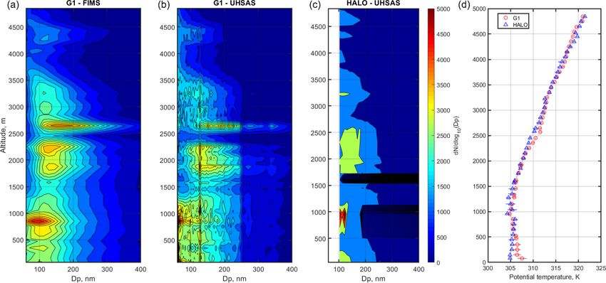
both UHSAS instruments was changed. Both the CPC and Figure 11 shows the vertical profiles of the aerosol mass
UHSAS measurement comparisons show stronger variation concentrations measured by the two AMSs on 21 Septem-
at the low altitude, especially below 2000 m. Above 3500 m, ber. The upper panel shows the medians and interquartile
the variations on the CPC- and UHSAS-measured concen- ranges of the different species (organics, nitrate, sulfate, am-
tration became significantly smaller than the variation at the monium) and the total mass concentration for the G1 (circles)
lower altitude. This result is consistent with the observation and HALO (triangles). The lower panel shows the difference
from the trace gas measurement and confirms that the vari- between the medians of G1 and HALO. The error bars were
ability of aerosol properties changes significantly with time calculated using error propagation from√ the error of the me-
and space. It is noticeable that the discrepancy observed in dian (interquartile range divided by 2 × N). The data were
the UHSAS measurement comparison is larger than that in grouped into 400 m altitude bins. The total mass concentra-
the CPC comparison. That is because the aerosol flow con- tion is the highest in the lower altitudes between 100 and
trol inside the UHSAS cannot respond quickly enough to 2000 m with a median value of 5 µg m−3 (G1-AMS). At alti-
the rapid change of the altitude and caused significant un- tudes between 2000 and 3800 m, the aerosol mass concentra-
certainty in the data. tion decreased to a median value of 1.2 µg m−3 (G1-AMS).
The most significant difference was observed at altitudes
3.3.2 Aerosol particle size distribution below 1800 m. The aerosol mass concentration measured by
HALO-AMS is less than that measured by G1 AMS, likely
For the cloud-free coordinated flight on 9 September, the av- due to particle losses in the constant pressure inlet (CPI) used
eraged aerosol size distributions measured by FIMS, G1 UH- on the HALO AMS. Between 1800 and 3000 m, the mass
SAS, and HALO UHSAS during one flight leg are compared concentrations measured by the HALO AMS exceed those
in Fig. 9. For particle diameter below 90 nm, the G1 UHSAS measured by the G1-AMS. This is most likely because the
overestimated the particle concentration, which is due to the G1 was sampling different air masses from the HALO, as in-
uncertainty in counting efficiency correction. The UHSAS dicated by the differences in CO mixing ratios and the CPC
detection efficiency is close to 100 % for particles larger than concentrations for this altitude region (see Figs. 5 and 8).
100 nm and concentrations below 3000 cm−3 but decreases Above 3000 m altitude, both instruments agree within the un-
considerably for both smaller particles and higher concentra- certainty range.
tions (Cai et al., 2008). The aerosol counting efficiency cor- Among individual species, the largest difference above
rection developed under the lab conditions does not necessar- 2000 m is observed for ammonium. The deployed G1 AMS
ily apply under the conditions during the flight. Between 90 is a high-resolution mass spectrometer (HR-ToF), whereas
and 250 nm, FIMS agreed well with the G1 UHSAS, whereas the HALO AMS has a lower resolution (C-ToF). The higher
HALO UHSAS was about 30 % higher than the two instru- resolution of the G1-AMS allows for a better separation of
ments. For the size range of 250–500 nm, FIMS had good interfering ions at m/z 15, 16, and 17 (NH+ , NH2+ , and
Atmos. Meas. Tech., 13, 661–684, 2020 www.atmos-meas-tech.net/13/661/2020/F. Mei et al.: Comparison of aircraft measurements 673
Figure 8. The G1 and HALO comparison for aerosol number concentration profiling measured by (a) CPC and (b) UHSAS (100–700 nm)
on 21 September.
found for a second comparison flight on 1 October 2014 (see
Sect. S2 and Figs. S7, S8).
3.3.4 CCN number concentration
These measurements provide key information about
aerosols’ ability to form cloud droplets and thereby modify
the microphysical properties of clouds. Numerous labo-
ratory and field studies have improved the understanding
of the connections among aerosol particle size, chemical
composition, mixing states, and CCN activation properties
(Bhattu and Tripathi, 2015; Broekhuizen et al., 2006; Chang
et al., 2010; Duplissy et al., 2008; Lambe et al., 2011; Mei
et al., 2013a, b; Pöhlker et al., 2016; Thalman et al., 2017).
In addition, based on the simplified chemical composition
Figure 9. The G1 and HALO comparison for aerosol size distribu- and internal mixing state assumption, various CCN closure
tion measured by UHSAS (from both aircraft) and FIMS (on the studies have achieved success within ±20 % uncertainty
G1) on 9 September. for ambient aerosols (Broekhuizen et al., 2006; Mei et al.,
2013b; Rissler et al., 2004; Wang et al., 2008).
According to earlier studies (Gunthe et al., 2009; Pöhlker
et al., 2016; Roberts et al., 2001, 2002; Thalman et al., 2017),
the hygroscopicity (κCCN ) of CCN in the Amazon basin is
NH3+ ) and thereby a more reliable calculation of the am- usually dominated by organic components (κOrg ). Long-term
monium mass concentration. ground-based measurements at the Amazon Tall Tower Ob-
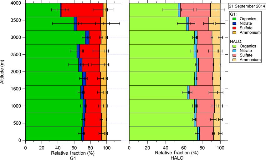
Overall, the aerosol chemical composition is dominated servatory also suggest low temporal variability and lack of
by organics, as is evident from the vertical profiles of the pronounced diurnal cycles in hygroscopicity only under nat-
relative fractions (Fig. 12). Both AMSs show a dominant ural rainforest background conditions (Pöhlker et al., 2016,
contribution of organics to the total mass concentration with 2018).
values around 70 %. This contribution is constant at alti- Using FIMS and CCN data from both the G1 and HALO
tudes between 100 and 3500 m and decreases to 50 % at collected during the coordinated flight leg on 9 September,
3800 m altitude. The inorganic fraction has the highest con- the critical activation dry diameter (D50 ) was determined by
tribution from sulfate (20 %), followed by ammonium (7 %) integrating FIMS size distribution to match the CCN total
and nitrate (2 %–4 %). For organics, ammonium, and sul- number concentration (Sect. S3). Then, the effective particle
fate, both instruments give similar relative fractions, only for hygroscopicity was derived from D50 and the CCN-operated
nitrate where a discrepancy is observed between 1000 and supersaturation using the κ-Köhler theory. The histogram
3000 m. Although the absolute aerosol mass concentration plots based on the density of the estimated hygroscopicity
measured by the HALO-AMS was affected by the constant (κest ) from both aircraft were compared for the flight leg
pressure inlet below 1800 m altitude, the relative fractions of above T3. The κest values derived from the G1 and HALO
both instruments generally agree well. Similar results were measurements during the flight leg above the T3 site are
www.atmos-meas-tech.net/13/661/2020/ Atmos. Meas. Tech., 13, 661–684, 2020You can also read