New in situ aerosol hyperspectral optical measurements over 300-700 nm - Part 2: Extinction, total absorption, water- and methanol-soluble ...
←
→
Page content transcription
If your browser does not render page correctly, please read the page content below
Atmos. Meas. Tech., 14, 715–736, 2021
https://doi.org/10.5194/amt-14-715-2021
© Author(s) 2021. This work is distributed under
the Creative Commons Attribution 4.0 License.

New in situ aerosol hyperspectral optical measurements over
300–700 nm – Part 2: Extinction, total absorption, water-
and methanol-soluble absorption observed during
the KORUS-OC cruise
Carolyn E. Jordan1,2 , Ryan M. Stauffer3 , Brian T. Lamb4 , Michael Novak3,5 , Antonio Mannino3 , Ewan C. Crosbie2,6 ,
Gregory L. Schuster2 , Richard H. Moore2 , Charles H. Hudgins2 , Kenneth L. Thornhill2,6 , Edward L. Winstead2,6 ,
Bruce E. Anderson2 , Robert F. Martin2 , Michael A. Shook2 , Luke D. Ziemba2 , Andreas J. Beyersdorf2,7 ,
Claire E. Robinson2,6 , Chelsea A. Corr2,8 , and Maria A. Tzortziou3,4
1 National Institute of Aerospace, Hampton, Virginia, USA
2 NASA   Langley Research Center, Hampton, Virginia, USA
3 NASA Goddard Space Flight Center, Greenbelt, Maryland, USA
4 Earth and Atmospheric Sciences, City University of New York, New York, New York, USA
5 Science Systems and Applications Inc., Lanham, Maryland, USA
6 Science Systems and Applications Inc., Hampton, Virginia, USA
7 Chemistry and Biochemistry, California State University, San Bernardino, San Bernardino, California, USA
8 Springfield College, Springfield, Massachusetts, USA

Correspondence: Carolyn E. Jordan (carolyn.jordan@nasa.gov)

Received: 7 August 2020 – Discussion started: 19 August 2020
Revised: 20 November 2020 – Accepted: 30 November 2020 – Published: 29 January 2021

Abstract. This two-part study explores hyperspectral (300–          scattering albedo (ω) was calculated. Water-soluble aerosol
700 nm) aerosol optical measurements obtained from in situ          composition from the DI extracts was used to examine re-
sampling methods employed during the May–June 2016                  lationships with the various measured optical properties. In
Korea–United States Ocean Color (KORUS-OC) cruise con-              particular, both σDI-abs (365 nm) and σMeOH-abs (365 nm) were
ducted in concert with the broader air quality campaign             found to be best correlated with oxalate (C2 O42− ), but el-
(KORUS-AQ). Part 1 focused on the hyperspectral measure-            evated soluble absorption was found from two chemically
ment of extinction coefficients (σext ) using the recently devel-   and optically distinct populations of aerosols. The more pho-
oped in situ Spectral Aerosol Extinction (SpEx) instrument          tochemically aged aerosols of those two groups exhibited
and showed that second-order polynomials provided a better          partial spectra (i.e., the longer wavelengths of the spectral
fit to the measured spectra than power law fits. Two dimen-         range were below detection) while the less-aged aerosol of
sional mapping of the second-order polynomial coefficients          the other group exhibited complete spectra across the wave-
(a1 , a2 ) was used to explore the information content of the       length range. The chromophores of these groups may have
spectra. Part 2 expands on that work by applying a similar          derived from different sources and/or atmospheric processes,
analytical approach to filter-based measurements of aerosol         such that photochemical age may have been only one factor
hyperspectral total absorption (σabs ) and soluble absorption       contributing to the differences in the observed spectra. The
from filters extracted with either deionized water (σDI-abs ) or    differences in the spectral properties of these groups was ev-
methanol (σMeOH-abs ). As was found for σext , second-order         ident in (a1 , a2 ) maps. The results of the two-dimensional
polynomials provided a better fit to all three absorption spec-     mapping shown in Parts 1 and 2 suggest that this spec-
tra sets. Averaging the measured σext from Part 1 over the          tral characterization may offer new methods to relate in situ
filter sampling intervals in this work, hyperspectral single-       aerosol optical properties to their chemical and microphysi-

Published by Copernicus Publications on behalf of the European Geosciences Union.
716                                                  C. E. Jordan et al.: In situ aerosol hyperspectral optical measurements

cal characteristics. However, a key finding of this work is that   field of regard of the Geostationary Ocean Color Imager
mathematical functions (whether power laws or second-order         (GOCI), which provided both hourly OC and aerosol op-
polynomials) extrapolated from a few wavelengths or a sub-         tical depth (AOD) observations from South Korea’s Com-
range of wavelengths fail to reproduce the measured spectra        munication, Ocean, and Meteorological Satellite (COMS).
over the full 300–700 nm wavelength range. Further, the σabs       The in situ aerosol measurement suite included both high-
and ω spectra exhibited distinctive spectral features across       temporal-resolution measurements (detailed in Part 1) and
the UV and visible wavelength range that simple functions          longer-duration filter sampling described in this work. Two
and extrapolations cannot reproduce. These results show that       sets of filters were collected for post-cruise analyses. The
in situ hyperspectral measurements provide valuable new            Teflon filters were extracted with water and methanol for
data that can be probed for additional information relating        subsequent composition and soluble absorption spectra mea-
in situ aerosol optical properties to the underlying physico-      surements. The glass fiber filters were placed in the center of
chemical properties of ambient aerosols. It is anticipated that    an integrating sphere to measure total aerosol absorption fol-
future studies examining in situ aerosol hyperspectral prop-       lowing the International Ocean Colour Coordinating Group
erties will not only improve our ability to use optical data       (IOCCG) protocol (IOCCG Protocol Series, 2018).
to characterize aerosol physicochemical properties, but that          Spectral measurements of soluble chromophores have be-
such in situ tools will be needed to validate hyperspectral re-    come routine for the characterization of brown carbon (BrC)
mote sensors planned for space-based observing platforms.          in the ambient atmosphere (e.g., Hecobian et al., 2010; Zhang
                                                                   et al., 2013, 2017); however, spectral measurements of to-
                                                                   tal aerosol absorption have not. Here, the approach devel-
                                                                   oped by the ocean color community (IOCCG Protocol Se-
1   Introduction                                                   ries, 2018) has been adopted to assess its applicability to
                                                                   atmospheric aerosols. This is similar to previously reported
In Part 1 (Jordan et al., 2021) of this two-part work, hyper-      measurements from particulates filtered from the meltwater
spectral aerosol extinction (σext ) measurements from a field      of ice and snow (Grenfell et al., 2011) in that ocean (and
campaign in South Korea were used to examine the useful-           freshwater) samples are filtered through glass fiber filters col-
ness of characterizing the spectra with second-order polyno-       lecting suspended particulates ranging from about 0.7–50 µm
mial rather than traditional linear fits (i.e., power laws with    (Stramski et al., 2015) on the filters. The filter is then placed
negative slopes known as Ångström exponents) to the log-           in the center of an integrating sphere attached to a spectrom-
arithmically transformed spectra. It was found that second-        eter to measure the absorption coefficient (σabs ) spectra of
order polynomials provided better fits to the data and that        the particulates. Here, we report hyperspectral measurements
using the two-coefficient mapping approach introduced by           from 300–700 nm (in common with the range reported in
Schuster et al. (2006) holds promise for providing more de-        Part 1 from the in situ Spectral Aerosol Extinction (SpEx)
tailed information on ambient aerosol size distributions than      instrument) for σabs and the two sets of soluble (deionized
can be obtained from single Ångström exponents alone. Fur-         water, DI; and methanol, MeOH) absorption spectra, σDI-abs
ther, it was demonstrated that extrapolating to wavelengths        and σMeOH-abs .
outside of the measurement range using either fitting ap-             Ocean particulates extend to much larger diameters than
proach can lead to large errors in calculated extinctions, sug-    atmospheric aerosols and exhibit complex absorption spec-
gesting that hyperspectral measurements over broad wave-           tra with features that include those that arise from specific
length ranges are preferable to Ångström-exponent-based ex-        pigments and physiological state of algae, along with the
trapolations. Here, we extend that work to examine the ap-         spectral dependence of non-algal particles such as suspended
plicability of second-order polynomials to represent hyper-        minerals and black carbon (BC) (e.g., Roesler and Perry,
spectral aerosol absorption measurements and whether two-          1995; Stramski et al., 2015; Mouw et al., 2015; IOCCG Pro-
coefficient mapping can provide more detailed information          tocol Series, 2018). The IOCCG (2018) measurement pro-
on aerosol composition derived from optical measurements           tocol is known as the quantitative filter technique (QFT,
compared to that from Ångström exponents.                          Mitchell, 1990; Röttgers and Gehnke, 2012; Stramski et al.,
   The data reported in this study are in situ aerosol mea-        2015) because it obtains quantitative σabs via an empiri-
surements (Table 1) from a suite of instruments deployed           cally derived correction factor. As discussed in Grenfell et al.
aboard the R/V Onnuri during the Korea–United States               (2011), Stramski et al. (2015), and IOCCG (2018) it is im-
Ocean Color (KORUS-OC; US-Korean Steering Group,                   portant that the particulates used to derive the correction are
2015) cruise around the Korean peninsula (20 May to 6 June         representative of the particulates present in the sample popu-
in 2016). In conjunction with the airborne air quality mis-        lation. As will be discussed further in Sect. 2.3, the difference
sion KORUS-AQ (Al Saadi et al., 2015; Crawford et al.,             between the size distribution and composition of atmospheric
2020; Tzortziou et al. 2018; Thompson et al. 2019), these          and oceanic particulates suggests that the IOCCG (2018) cor-
field campaigns were joint South Korean–United States mis-         rection factor may not be applicable to this sample set. How-
sions to investigate ocean color and air quality within the        ever, with a suitably adjusted correction, this method allows

Atmos. Meas. Tech., 14, 715–736, 2021                                                 https://doi.org/10.5194/amt-14-715-2021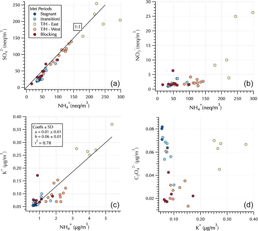
C. E. Jordan et al.: In situ aerosol hyperspectral optical measurements                                                                                                            717

Table 1. Summary of measurements in this study with estimated measurement errors.

    Measurement method                                        Parameter                                                                          Estimated measurement
                                                                                                                                                 error
    In situ Spectral Aerosol                                  Aerosol extinction coefficients (σext )                                            ∼5%
    Extinction instrument (SpEx)                                                                                                                 (300–700 nm)a
    AirPhoton IN101 nephelometer                              Aerosol scattering coefficients (σscat )                                           < 1 Mm−1
                                                              at 450, 532, and 632 nm                                                            (all wavelengths)b
    Brechtel Tricolor Absorption                              Aerosol absorption coefficients (σabs )                                            ∼ 0.2 Mm−1
    Photometer (TAP)                                          at 467, 528, and 652 nm                                                            (based on 60 s means,
                                                                                                                                                 all wavelengths)c
    Glass fiber filter in integrating                         Total aerosol absorption                                                           ∼ 17 %
    sphere attached to dual-                                  coefficients (σabs )                                                               (300–700 nm)d
    beam spectrophotometer
    Teflon filter extracts in liquid waveguide
    capillary cell using two solvents:
       – methanol (MeOH)                                      MeOH-soluble aerosol absorption coefficients (σMeOH-abs )                          ± 30 %e
       – deionized 18 M water (DI)                           DI-soluble aerosol absorption coefficients (σDI-abs )                              ± 30 %e
                                                                                              2−
    Ion chromatography of DI extracts                         NH+     +    2+    2+     +             −   −
                                                                 4 , K , Ca , Mg , Na , SO4 , NO3 , Cl , and                                     ± 30 %e
                                                                  2−
                                                              C2 O4 (mass and equivalents concentrations)

    Aerosol mass spectrometry of                              Organics, sulfate, nitrate, ammonium, and chloride                                 ± 30 %e,f
    DI extracts                                               (relative contributions to a sample)
  a Jordan et al. (2015, 2021). b Operating Manual for Sampling Station and Nephelometer, version 1.1, February 2014 (AirPhoton, Baltimore, MD). c Brechtel TAP Tricolor
  Absorption Photometer Model 2901 System Manual Revision 1, 24 June 2015 (Brechtel, Hayward, CA). d Estimated from propagation of uncertainty as discussed in
  Sect. 2.3. e Uncertainty in the extraction volume was the dominant term in error propagation, leading to somewhat-greater-than-typical estimated errors in the data from
  solvent extracts. f As discussed in Sect. 2.5 it is not possible to derive mass concentrations for the AMS data reported here; hence, the estimated error reflects that of the
  other solvent extract data for consistency.

for quantitative measurements of aerosol σabs spectra that can                                hematite and goethite, exhibit very different wavelength de-
be combined with σext spectra (as described in Part 1) for the                                pendence in their absorption spectra (Schuster et al., 2016).
calculation of hyperspectral single-scattering albedo (ω).                                       Given the importance of composition on the absorption of
   The ability of aerosols to absorb light depends on their                                   aerosols, it is not uncommon to treat σabs as a function of
molecular structure, specifically the presence of conjugated                                  composition, while treating σscat (and by extension σext , since
(or π) bonds, heteroatoms (e.g., N or O), and functional-                                     scattering is the dominant term in extinction) as a function of
group molecular structures (e.g., Jacobson, 1999; Apicella                                    aerosol size distribution. This separation is not strictly true
et al., 2004; Andreae and Gelencsér, 2006; Moosmüller et al.,                                 as mixing state and size distributions have been shown to in-
2009; Chen and Bond, 2010; Desyaterik et al., 2013). The                                      fluence the spectral behavior of σabs (Schuster et al., 2016),
number of such structures determines the wavelength de-                                       while absorption has been shown to influence the spectral
pendence of the absorption spectrum, such that more ab-                                       behavior of σext (Eck et al., 2001). Hence, the ability to si-
sorbing molecular structures allow for absorption across a                                    multaneously measure hyperspectral σabs and σext of in situ
wider range of wavelengths. In the graphitic sheets that com-                                 aerosols along with their chemical composition and size dis-
prise BC there are so many π bonds that light is absorbed                                     tributions is anticipated to improve our understanding of the
throughout the ultraviolet (UV)–visible (Vis)–infrared (IR)                                   interaction of differing spectral dependencies due to various
range (e.g., Yang et al., 2009; Desyaterik et al., 2013; Bond                                 microphysical aspects of ambient aerosols.
et al., 2013). Organic aerosols, however, contain far fewer                                      For KORUS-OC, the in situ aerosol instrument suite did
such structures such that light is absorbed only over a por-                                  not include size distribution measurements or online com-
tion of the UV–Vis–IR range and may not exhibit absorp-                                       position; however, there is extensive information about the
tion in the Vis–IR at all. Non-carbonaceous aerosols, such                                    ambient aerosols observed throughout the KORUS-AQ cam-
as dust, are also known to weakly absorb light as a func-                                     paign that can be used to assess how the ambient aerosol sizes
tion of their composition, principally according to their pro-                                and composition influenced the observed spectral character-
portion of iron oxides (e.g., Sokolik and Toon, 1999; Moos-                                   istics obtained from the instruments aboard the R/V Onnuri.
müller et al., 2012; Shi et al., 2012). Two forms of iron oxide,                              As will be discussed in Sects. 2.1 and 3.2, there were three

https://doi.org/10.5194/amt-14-715-2021                                                                                    Atmos. Meas. Tech., 14, 715–736, 2021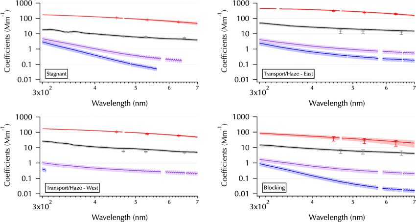
718                                                      C. E. Jordan et al.: In situ aerosol hyperspectral optical measurements

Figure 1. Map of mean sampling locations for the filter data set colored by the Peterson et al. (2019) meteorological regimes with Trans-
port/Haze data split between upwind (west, orange) and downwind (east, yellow) positions around the peninsula. Error bars represent 1 SD
of the mean filter sample latitude and longitude, used to distinguish filters collected on station from those collected underway. See Table S1
for details.

distinct synoptic meteorological periods during the KORUS-               shown in Fig. 1 (see Table S1 in the Supplement for details
OC cruise (Peterson et al., 2019) that gave rise to aerosol              as some filter samples overlap in the figure). The locations
populations that differed in size and composition (Jordan                shown in Fig. 1 are color-coded according to the meteoro-
et al., 2020, 2021). These different ambient populations pro-            logical regimes during the cruise as described by Peterson
vide the framework that will be used here to assess shifts in            et al. (2019): Stagnant (17–22 May, under a persistent anti-
the optical properties related to size distribution (σext , follow-      cyclone), Transport/Haze (25–31 May, dynamic meteorology
ing the discussion in Part 1) and composition (σabs , σDI-abs ,          with four frontal passages, westerly low-level transport from
and σMeOH-abs ).                                                         upwind sources in China, and humid conditions promoting
                                                                         the development of fog and haze under cloudy skies), and
                                                                         Blocking (1–7 June, less persistent stagnation arising from
2     Methods                                                            a Rex block, i.e., adjacent high- and low-pressure systems
                                                                         with the high poleward of the low) with periods nominally
2.1    Ship deployment and high-frequency, ambient
                                                                         defined from midnight (00:00) through midnight (24:00) lo-
       aerosol measurements
                                                                         cal time. Note that in Fig. 1 there is a group of filter samples
A detailed description of the ship deployment and the high-              classified as “transition” collected on 23 and 24 May as the
frequency measurements made as part of the in situ aerosol               Stagnant period meteorological conditions gave way to those
instrument suite deployed on the Korean Institute of Ocean               that defined the Transport/Haze period. Following the dis-
Sciences and Technology (KIOST) R/V Onnuri is provided                   cussion in the companion paper, the Transport/Haze filter set
in the companion paper (Jordan et al., 2021). In brief, the              is divided into two subsets, those downwind of the Korean
KORUS-OC cruise of the R/V Onnuri sailed first along the                 peninsula along the east coast and those upwind to the west
east coast of South Korea and then transited to the west                 of the peninsula with the one sample along the south coast as-
(Fig. 1). The in situ aerosol instrument suite measured fine-            signed to the west group. Details on the specific meteorolog-
mode aerosols with a 50 % cutoff size of 1.3 µm diame-                   ical conditions and aerosol characteristics will be discussed
ter. Filter samples were collected over 3 h daytime intervals,           in Sect. 3.2.
along with a 12 h overnight sample, each day from 22 May                    Means for each filter sampling interval (Table S1) were
to 4 June (local Korea standard time, KST, = UTC + 9) out-               calculated from high-temporal-resolution data sets described
side of the South Korea’s territorial waters (> 12 nautical              in Jordan et al. (2021): three-visible-wavelength scattering
miles, 22.2 km, from the coast) with mean sampling locations             (450, 532, and 632 nm σscat , AirPhoton IN101 nephelome-

Atmos. Meas. Tech., 14, 715–736, 2021                                                        https://doi.org/10.5194/amt-14-715-2021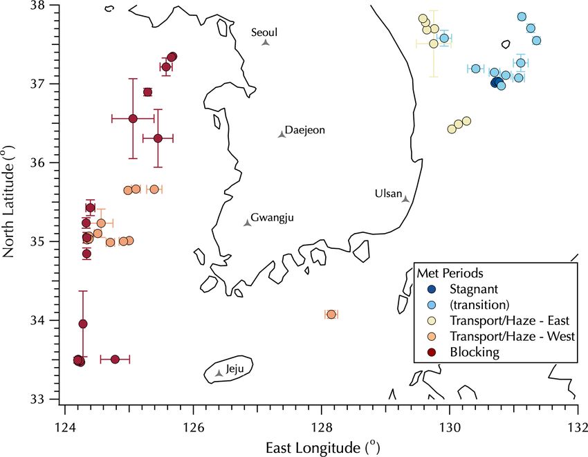
C. E. Jordan et al.: In situ aerosol hyperspectral optical measurements                                                        719

ter, Baltimore, MD) and absorption (467, 528, and 652 nm            sette for sampling aboard ship. The two filter cassettes sam-
σabs , Tricolor Absorption Photometer, TAP, Brechtel, Hay-          pled in parallel off the common inlet used for the measure-
ward, CA), and hyperspectral σext (300–700 nm) from the             ment suite. The flow rates through the Teflon and GF/F fil-
custom-built SpEx instrument. Filter mean σext calculated at        ters were ∼ 24 and ∼ 21 L m−1 , respectively. After sampling,
450, 532, and 632 nm (see Jordan et al., 2021, for details)         filters were individually placed in polystyrene petri dishes,
from the σscat and σabs data is denoted NT σext here, in con-       sealed with Teflon tape, wrapped in aluminum foil to limit
trast to SpEx σext . The high-resolution data set was flagged to    exposure to light, placed in Ziploc bags, and kept frozen un-
identify and remove interceptions of the R/V Onnuri’s own           til they were analyzed in the laboratory.
ship stack emissions (Jordan et al., 2021). Similarly, here it
was also used to assess potential ship plume contamination
of the filter set (see the discussion in the Supplement). Of the    2.3   Total absorption coefficient spectra from GF/F
53 pairs of filters collected, no ship plume interceptions oc-            samples
curred for 15. The degree of contamination depended on the
duration of the interception as well as on the aerosol prop-
erty of interest (e.g., Fig. S1 in the Supplement), such that       Total absorption coefficient (σabs ) spectra from 300–700 nm
in the few instances where the plume contamination (PF1,            at 0.2 nm spectral resolution were obtained from the GF/F
gray plus symbols) values in scattering or absorption were          set by placing each filter in the center of an integrating
relatively large their influence over the filter sampling inter-    sphere (Labsphere DRA-CA-30) attached to a dual-beam
val was small (compare the solid, all data, and open, PF0,          spectrophotometer (Cary 100 Bio UV–visible spectropho-
green symbols in Fig. S1). Here, single-scattering albedo cal-      tometer). This methodology is well established in the ocean
culated from IN101 and TAP data provided the most conser-           color community for obtaining particulate σabs spectra from
vative delineation between ambient and ship plume aerosol           filtered water samples (e.g., Stramski et al., 2015; Neeley
(Figs. S1 and S2), resulting in 13 of the filter pairs being        et al., 2015; IOCCG Protocol Series, 2018). The GF/F set
rejected (Table S2) from most of the analyses presented in          was collected during KORUS-OC to test the applicability of
Sect. 3 (except as noted). Given the generally small differ-        this approach to atmospheric aerosol samples.
ence in absorption resulting from the ship plume intercep-              The absorbance spectra of the GF/F filter set were mea-
tions, all but filter 22 were retained for the assessment of        sured in the laboratory over the course of 4 d with regular air
the correction factor for the spectral absorption measurement       scans (spectra obtained with the filter holder in the integrat-
discussed in Sect. 2.3. Although, filter 22 was rejected from       ing sphere without a filter in place) measured to account for
further analyses on the basis of ship plume contamination           any drift in the spectrophotometer measurement. Absorbance
(Table S2), this particular filter was also so heavily loaded       spectra from field blank filters were consistent with labo-
due to polluted ambient conditions that the measured spec-          ratory blank filters indicating that handling in the field did
trum in the integrating sphere was distorted. Hence, this fil-      not contribute to the measured absorbance of the sample fil-
ter was also excluded from the calculation of the correction        ters. Blank corrections for the sample filters were calculated
factor on the basis of its being overloaded.                        by taking the mean of the air scans and subtracting it from
                                                                    the mean of the field blank spectra. Multiple scans (2–6) for
2.2   Filter preparation and sampling procedures                    each filter sample were performed, rotating the filter position
                                                                    between scans to assess variability in the measurement by
Two sets of filters were collected for subsequent spectral          sampling different parts of the filter with the narrow, colli-
analyses in the laboratory: glass fiber filters (Whatman GF/F       mated beam. The mean spectrum was then blank corrected.
47 mm filters, 0.7 µm pore size) for total absorption spectra       Two lamps are used in the spectrophotometer to cover the
(σabs ) measured in an integrating sphere attached to a spec-       full spectral range. The tungsten (halogen) lamp provides a
trophotometer (see Sect. 2.3 below) and Teflon filters (Flu-        stable signal that spans most of the spectral range. Scanning
oropore PTFE 47 mm filters, 1 µm pore size) for soluble ab-         from longer to shorter wavelengths at 350 nm the instrument
sorption spectra from deionized water (σDI-abs ) and methanol       switches to a much noisier deuterium lamp to cover the re-
(σMeOH-abs ) extracts from the filters (see Sect. 2.4 below). For   mainder of the UV range where the intensity of the tungsten
each filter set, a blank filter was collected each day during the   light source is too low to make a good measurement. To min-
cruise by briefly putting it in the sampling line without any       imize the noise present in the UV, a 10 nm boxcar smooth-
airflow through the system.                                         ing algorithm was applied to the full wavelength range of
   The Teflon filters were taken directly from their pack-          the 0.2 nm scans. The lower limit of detection (LLOD) for
age and placed in a filter cassette for sampling. GF/F filters      the sample data set was calculated from the mean +3 SDs of
were pre-baked at 450 ◦ C for 6 h in the laboratory prior to        the field blank filters. Measurement error for the absorbance
the cruise. They were then individually stored in polystyrene       scans was estimated to be about 15 %.
petri dishes sealed with Teflon tape, wrapped in aluminum               The dimensionless blank-corrected absorbance (Abs, also
foil, and enclosed in Ziploc bags until placed in a filter cas-     known as the spectral optical density of the filter; Stramski

https://doi.org/10.5194/amt-14-715-2021                                                 Atmos. Meas. Tech., 14, 715–736, 2021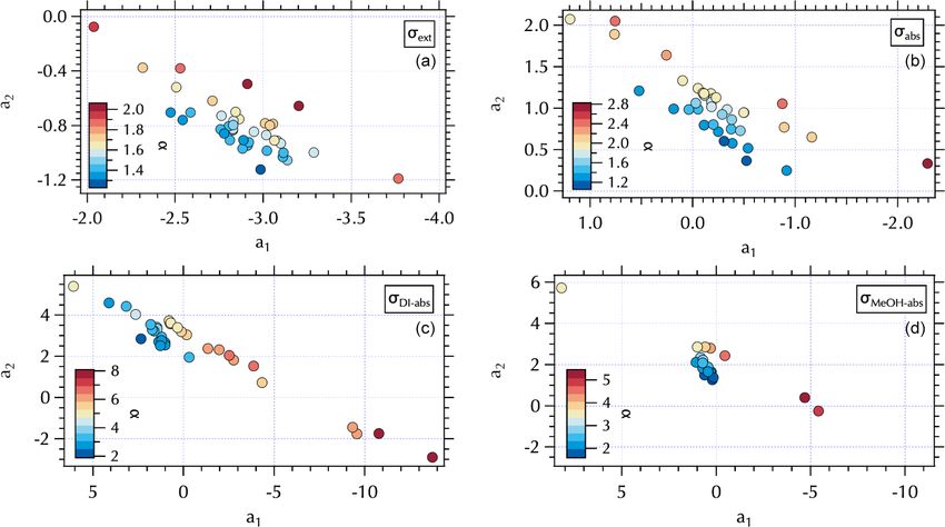
720                                                    C. E. Jordan et al.: In situ aerosol hyperspectral optical measurements

et al., 2015) is then used to calculate the σabs via                 correction (Ogren et al., 2017) suitable for atmospheric BC
                                                                     aerosols, along with the known importance of using a β cor-
             LN(10) · Abs(λ) · fa
σabs (λ) =                        ,                           (1)    rection determined from particles representative of the sam-
                  Vair · β                                           ple data, we have greater confidence in the magnitude of the
                                                                     TAP values than the βs correction for this data set. Empiri-
where fa is the area of the filter (in m2 ), Vair is the volume of
                                                                     cally determining an appropriate β for the samples obtained
air sampled through that filter area (in m3 ), β is a term used to
                                                                     in this study was beyond the scope of this project. However,
correct for pathlength amplification of the signal by the filter
                                                                     taking advantage of the TAP data set, β for the KORUS-OC
and collected particles (Butler, 1962; Kiefer and Soo Hoo,
                                                                     data (βK-OC ) was obtained by scaling βs to fit the TAP data
1982; Kishino et al., 1985), and the LN(10) term converts
                                                                     (βK-OC = 0.593 · βs = 1.836 · Abs−0.0867 ; see Fig. S3) result-
the base 10 logarithm absorbance measurement (= −log10 T ,
                                                                     ing in quantitative σabs spectra. Error propagation (i.e., the
where T is transmittance) to a natural logarithm as used for
                                                                     propagation of the uncertainty of each term in Eq. 1) was
ambient environmental observations. These terms result in
                                                                     used to estimate the uncertainty in the σabs spectra (Eq. 1)
units of m−1 for σabs (λ), which are inconvenient for atmo-
                                                                     from the estimated 15 % error of the absorbance spectra, the
spheric data. Hence, an additional factor of 106 is also used
                                                                     SD of the slope (± 0.034) used to estimate βK-OC , the uncer-
to convert the units to Mm−1 for the data set herein. The
                                                                     tainty in the filter area (based on ± 1 mm in diameter of the
β correction accounts for the scattering enhancement by the
                                                                     estimated filter sampling diameter of 42.6 mm of the 47 mm
fibers within the filter itself, as well as by the particles col-
                                                                     diameter filters), and the SD of the mean volume of air sam-
lected on and within the filter medium, and is defined as the
                                                                     pled for each filter calculated from 1 s flow rate data. Over
ratio of the measured filter absorbance to the true absorbance
                                                                     300–700 nm the estimated error in σabs is ∼ 17 % (Table 1).
of the sample.
                                                                        The spectrometers used to measure σext and σabs had
   β has been determined empirically with the standard pro-
                                                                     different spectral resolutions. Hence, in order to calculate
tocol (IOCCG Protocol Series, 2018) adopting the parame-
                                                                     single-scattering albedo (ω) these spectra sets were averaged
terization determined by Stramski et al. (2015), denoted here
                                                                     into 2 nm bins over 300–700 nm. Then spectral ω was calcu-
as βs ,
                                                                     lated via
βs = 3.096 · Abs−0.0867 .                                     (2)             σext (λ) − σabs (λ)
                                                                     ω(λ) =                       .                             (3)
The ocean optics and biogeochemistry protocol (IOCCG                                σext (λ)
Protocol Series, 2018) notes that “understanding . . . the           2.4   Soluble absorption coefficient spectra from Teflon
types of particle assemblages for which the formulated path-               samples
length amplification correction is representative” is impor-
tant. Here, those assemblages included nearshore mineral-            The Teflon filters were cut in half in order to extract water-
dominated and red tide samples, mixtures of phytoplankton            soluble aerosol components from one half that could be fur-
species, and other coastal and offshore particle assemblages         ther analyzed via ion chromatography and aerosol mass spec-
spanning a size range of about 0.7 to 50 µm (Stramski et al.,        trometry (see Sect. 2.5) and non-water-soluble components
2015). A similar study that used a different instrument con-         from the other half using an organic solvent. Here, methanol
figuration to measure the absorption of particles filtered from      (MeOH) was used for the organic solvent as both water
snow and ice meltwater (Grenfell et al., 2011) noted that the        and MeOH solutions were compatible with the waveguide
calibration standard used for soot was carefully filtered to re-     used to measure the absorbance of the dissolved aerosol
move particles that were too large to be representative of the       components in the extracts. Half of the filter was placed
ambient samples. Figure S3 shows the relationship between            in a clean 15 mL polypropylene centrifuge tube (Corning
σabs calculated using Eqs. (1) and (2) from the filter measure-      430052; triple rinsed, soaked overnight, and triple rinsed
ments in the integrating sphere compared to σabs measured            again with Milli-Q 18 M deionized (DI) water) and ex-
by TAP (values at 467, 528, and 652 nm wavelengths are               tracted in 10 mL of DI water by hand shaking the tube for
all plotted together here). Using no correction at all (β = 1)       60 s. Tests were performed that showed this method extracted
results in values much higher than the TAP values (with a            the soluble chromophores equally well as with 60 min of
slope of 2.361), while the βs correction leads to values that        sonication; hence the faster approach was employed. Ex-
are much lower (slope of 0.593).                                     tracts were filtered to remove any insoluble particles using
   Fresh soot particles from diesel engines are small, typi-         polypropylene Soft-Ject disposable 12 mL syringes (Henke-
cally on the order of tens of nanometers (Bond et al., 2013);        Sass, Wolf) and 0.2 µm pore size PTFE-membrane filters
hence the size range measured by the in situ aerosol instru-         (Cole-Parmer).
ment suite aboard R/V Onnuri (≤ 1.3 µm diameter) likely in-             The other half of the filter was placed in a clean 15 mL
cluded smaller particles (as well as particles with a very dif-      glass vial with a Teflon cap (rinsed with spectrophotometric-
ferent composition) than those used to derive βs . Given that        grade (≥ 99.9 %) MeOH (Sigma Aldrich product number
TAP is a commercial instrument with a well-characterized             154903) and dried in a fume hood) and extracted in 10 mL

Atmos. Meas. Tech., 14, 715–736, 2021                                                    https://doi.org/10.5194/amt-14-715-2021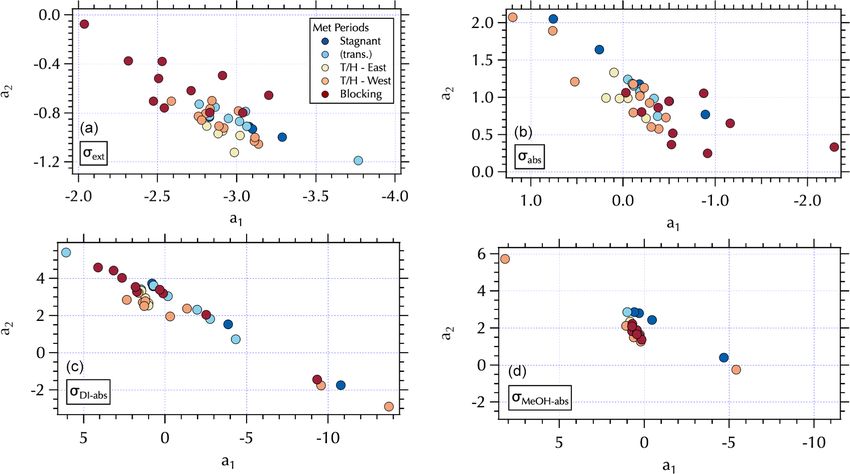
C. E. Jordan et al.: In situ aerosol hyperspectral optical measurements                                                           721

of MeOH by hand shaking the vial for 60 s. Extracts were                 σsol-abs for the soluble aerosol chromophores in the ex-
filtered to remove particles using a glass syringe with a             tracts were then calculated from the blank-corrected Abs
0.2 µm pore size PTFE-membrane filter (Cole-Parmer). Un-              spectra via
fortunately, some of the MeOH extracts vials were contam-
                                                                                                 Vs
inated during handling and are marked as “missing” in Ta-             σsol-abs (λ) = Abs(λ) ·          LN(10),                     (6)
ble S1. As a result, there are fewer MeOH-soluble absorption                                    Va · l
spectra in the data set than DI-soluble absorption spectra. In        where Vs is the volume of solvent used to extract the filter
all cases where there are both spectra, greater absorption was        (in liters), Va is the volume of air sampled by the filter (in
observed from the MeOH extracts.                                      liters), l is the absorbing path length of the capillary cell (in
    A liquid waveguide capillary cell (LWCC; World Preci-             meters), and LN(10) converts the base 10 log used for ab-
sion Instruments LWCC-3100, 100 cm pathlength) attached               sorbance to natural log typically used for atmospheric quan-
to an SM240 spectrometer (Spectral Products, Putnam, CT,              tities (Hecobian et al., 2010). Again, the units were converted
∼ 0.4 nm spectral resolution) with a DH-2000-BAL light                from m−1 to Mm−1 per the convention commonly used for
source (Ocean Optics, Dunedin, FL) operated with a 2 s inte-          atmospheric data sets. σsol-abs spectra are reported for the
gration time was used to measure the absorbance of the sol-           wavelength range of 300–700 nm with problematic wave-
uble aerosol chromophores in each filter extract. Note that           lengths (due to saturation of the detector) removed resulting
absorbance (Abs) is the measured quantity; it is not the same         in evident gaps in the spectra (e.g., Fig. 2). The uncertainty
as the absorption coefficient (σsol-abs , where the notation sol-     in σsol-abs (λ) was assessed using error propagation and found
abs is used to distinguish soluble from total absorption co-          to be about ± 30 %, principally due to the uncertainty in the
efficients). σsol-abs , the relevant atmospheric quantity, is de-     volume of the solvent used to extract the filters.
rived from Abs. The relationship between these values is ex-              Previous authors (e.g., Hecobian et al., 2010; Zhang et al.,
plained below. Each set of measurements in the laboratory             2013) have calculated σsol-abs (λ) at 365 nm (σsol-abs (365 nm))
started with a dark count spectrum followed by an alternat-           by averaging over the 360–370 nm range of the spectrum in
ing sequence of a reference spectrum from the solvent alone,          order to use it as a single value proxy for soluble organic
then a sample spectrum from a filter extract, then another            aerosol chromophores. This avoids contributions from inor-
reference spectrum, etc. Periodically, the LWCC would be              ganic nitrate absorption that occurs at wavelengths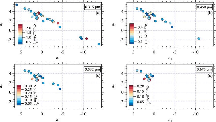
722                                                       C. E. Jordan et al.: In situ aerosol hyperspectral optical measurements

Figure 2. One example from each meteorological regime as shown in Fig. 1 of the spectra set obtained from each filter: mean SpEx σext (red
line, shaded with ± 1 SD), σabs (black line), and σMeOH-abs and σDI-abs (purple and blue lines, respectively). Measurement error for all of
the absorption coefficient spectra estimated using error propagation (shading, on a log scale this is more difficult to discern for σabs than for
σMeOH-abs and σDI-abs ). Mean NT σext (red symbols ± 1 SD) and mean TAP σabs (gray symbols ± 1 SD) are shown for comparison. All in
units of Mm−1 .

centrations of the aerosol components measured here with                   values examined was truncated to the m/z 12–73 range. For
the AMS. The nebulizers used to disperse the DI extracts into              all but six filters this captured ≥ 0.9 of Organics.
aerosols do so with an unknown liquid flow rate such that the
original atmospheric aerosol mass concentrations in ambi-
ent air cannot be calculated. Hence, in order to make com-                 3     Results and discussion
parisons across the data set, the AMS data are presented in
terms of ratios, either the ratio of the major chemical groups             3.1    Filter spectra set overview
(sulfate, ammonium, nitrate, chloride, and organic) to their
summed total mass (Total) or the ratio of individual m/z                   Each panel of Fig. 2 shows one filter from each meteoro-
groups to the total organic mass (Organics). Note that since               logical period as shown in Fig. 1 to illustrate differences ob-
organic sulfate and nitrate compounds can contribute to the                served across the entire data set. For the measured filter spec-
sulfate and nitrate measured by AMS the notation used for                  tra (σabs , black; σMeOH-abs , purple; and σDI-abs , blue, curves
ions is not used here. Throughout this paper the overlapping               in Fig. 2) shading is used to indicate estimated measurement
IC and AMS measurements are distinguished by using the                     errors in absorption coefficients (see Table 1) as described
ionic notation for the former (i.e., SO2−           −                      in Sect. 2. The larger errors for the soluble absorbers make
                                           4 and NO3 ) and the
terms (i.e., sulfate and nitrate) for the latter.                          this shading easier to discern than that for σabs on the log
   The summation over all m/z ≥ 12 used to calculate Organ-                scale needed here to show all of the spectra together. For the
ics included negative values that arise from the subtraction of            higher-temporal-resolution measurements averaged over the
a reference spectrum (filtered airflow to remove the particles)            filter sampling periods, shading (SpEx σext , red curves) and
from the unfiltered airflow containing aerosols in the AMS.                error bars (NT σext , red pluses, and TAP σabs , gray pluses)
Typically, the negative values were a minor contribution.                  indicate 1 SD of the mean. Hence, the SDs reflect the vari-
However, in some cases they were large. Hence, the frac-                   ability of the ambient atmosphere over each filter sampling
tional contributions of each m/z to the sum (denoted here as               period. For three of the examples, little ambient variability in
“f_m/z”) were normalized across only positive values. The                  σext was observed, while the example from the Blocking pe-
normalized value was used to approximate above-detection                   riod indicates rapidly changing conditions that occurred dur-
contributions for each m/z to Organics. Note that in the as-               ing the 12 h overnight sample from 1 to 2 June (see Part 1).
sessment of individual contributions to Organics the range of                  Key features to note in Fig. 2 include the spectral vari-
                                                                           ability in σabs , where sometimes it is smoothly varying (e.g.,
                                                                           Blocking) and sometimes there are spectral features evident

Atmos. Meas. Tech., 14, 715–736, 2021                                                          https://doi.org/10.5194/amt-14-715-2021
C. E. Jordan et al.: In situ aerosol hyperspectral optical measurements 723
(e.g., the UV portion of the Stagnant spectrum). The spectral ulations at the surface across South Korea (Jordan et al.,
features (i.e., enhanced absorption over a limited wavelength 2020) both in terms of composition and size distributions
range compared to the rest of the spectrum) likely arise from of fine-mode aerosols (i.e., particulate matter with diame-
specific molecular structures within the ambient aerosols that ters ≤ 2.5 µm, PM2.5 ). PM2.5 was most elevated during the
absorb light over a limited wavelength range as discussed Transport/Haze period, followed by the Stagnant period (Pe-
in the introduction. Also note the changing relationship be- terson et al., 2019). Stagnant conditions fostered the accu-
tween σMeOH-abs and σDI-abs , where they can be very similar mulation of locally photochemically produced secondary or-
across the spectrum (e.g., Transport/Haze – East) or diverge ganic aerosol (SOA) under clear skies (Kim et al., 2018;
substantially at longer wavelengths (e.g., Blocking). Finally, Nault et al., 2018; Choi et al., 2019; Peterson et al., 2019;
note the partial spectra for σMeOH-abs and σDI-abs , where only Jordan et al., 2020). During the Transport/Haze period trans-
a portion of the spectrum is above detection. These partial port from the west/northwest brought polluted air from China
spectra vary considerably in the above-detection wavelength to S. Korea under cloudy humid conditions that promoted
range with the Transport/Haze – West example showing an rapid local heterogeneous production of secondary inorganic
extreme case where all of the σMeOH-abs is above detection, aerosols (SIAs) within a shallow boundary layer producing
while little of the σDI-abs is above detection. In contrast, for the highest PM2.5 concentrations during KORUS-AQ (Peter-
the Stagnant example both of these spectra are partial but son et al., 2019; Eck et al., 2020; Jordan et al., 2020). During
span most of the wavelength range. The differences between this period PM2.5 was much greater than PM1 (i.e., aerosols
the spectra obtained from the DI and MeOH extracts for any with diameters ≤ 1 µm) at Olympic Park in Seoul, often by
given sample arise from differing solubilities of the chemi- 20–40 µg m−3 . In contrast, at the end of the Stagnant period
cal components of the aerosols in those two solvents. Differ- PM2.5 only exceeded PM1 by margins ≤ 10 µg m−3 (Jordan
ences in the soluble spectra across the sample set arise from et al., 2020). Hence, the size distributions as well as con-
differences in the ambient aerosol population across the me- centrations and compositions differed between these periods.
teorological regimes of the campaign. The Blocking period (limited transport, occasional brief stag-
DI extracts were analyzed for composition, enabling anal- nant periods, and rain to the south; Peterson et al., 2019) be-
yses to relate composition to optical properties as will be gan following a frontal passage that brought clean air from
discussed in Sect. 3.2. Also in that section, previously pub- the north. As discussed in the companion paper (Jordan et al.,
lished work from the KORUS-AQ campaign is used to pro- 2021), the fine-mode aerosols sampled aboard R/V Onnuri
vide greater context for the differences in the aerosol popula- during this period were likely due to small absorbing aerosols
tions sampled during the three meteorological regimes that from ship emissions in the West Sea.
occurred during the cruise. In Sect. 3.3 fits to the spectra The aerosol composition measured via the AMS from the
set from second-order polynomials are compared to those nebulized water-soluble filter extracts (Fig. 3) is consistent
from power laws. This section also includes a preliminary with the previously reported aerosol composition (Kim et al.,
examination of how the different aerosol populations map 2018; Nault et al., 2018, Choi et al., 2019; Peterson et al.,
into the two-parameter space described by the second-order 2019; Jordan et al., 2020). Dramatic shifts in composition
polynomial coefficients providing a potential avenue to relate across the differing meteorological regimes are evident in
aerosol physicochemical properties to spectral optical char- Fig. 3, with organics contributing 85 % to the total AMS
acteristics. In Sect. 3.4, single-scattering albedo (ω) spectra mass during the Stagnant period vs. 33 % and 45 % when the
calculated from σabs and σext are used to illustrate the spec- ship was downwind (25–27 May) and upwind (29–31 May),
tral features in σabs that more clearly manifest in ω. The in respectively, of the peninsula during the Transport/Haze pe-
situ aerosol instrument suite aboard the R/V Onnuri did not riod. There is also a clear shift in the water-soluble organic
include online aerosol composition measurements that could composition between the downwind and upwind sides of the
have been used to interpret the absorption features in the σabs peninsula with m/z 44 dominant downwind and m/z 43 con-
spectra limiting chemical attribution to the various features tributing a larger fraction to the organic mass on the upwind
observed. However, the examples provided show that fu- side (Fig. 3). m/z 44 is predominantly attributed to the CO+ 2
ture studies that combine hyperspectral total absorption with fragment originating from carboxylic acids, to which ox-
composition measurements that capture the total aerosol (not alate is a contributor, and is the basis for positive matrix fac-
just the water-soluble components) may enable such linkages torization (PMF) techniques to quantify secondary organic
to be made. aerosols (SOA; Zhang et al. 2005) and highly oxidized or-
ganic aerosol (i.e., OOA-1 from Ulbrich et al., 2009). m/z 43
3.2 Water-soluble aerosol composition and 365 nm results from both oxidized and aliphatic fragments, C2 H3 O+
optical properties compared across meteorological and C3 H+ 7 , respectively, and is enhanced relative to m/z 44
regimes during KORUS-OC for less-oxygenated organic aerosol (e.g., OOA-2 from Ul-
brich et al., 2009). Likewise, higher ratios of m/z 44 : 43
The synoptic meteorology of the KORUS-AQ campaign de- are indicative of lower volatility, more photochemically aged
scribed by Peterson et al. (2019) led to differing aerosol pop-
https://doi.org/10.5194/amt-14-715-2021 Atmos. Meas. Tech., 14, 715–736, 2021724 C. E. Jordan et al.: In situ aerosol hyperspectral optical measurements
Figure 3. The fraction contributed to the total mass measured by AMS by each of the major aerosol components (a) and the fraction of key
water-soluble organic mass fractions to the total AMS organic mass (b) for the complete filter set (Table S1) are shown within the context
of the Peterson et al. (2019) meteorological regimes. Note that the long gaps between filters during the Transport/Haze period occurred as
the ship transited South Korea’s territorial seas with samples obtained when the ship was outside of those waters. The single filter obtained
along the south coast (Fig. 1) is the isolated data point on 28 May. The Transport/Haze samples collected from 25–26 May were obtained
to the east of the peninsula, and those from 29–31 May were obtained to the west, representing downwind and upwind samples with respect
to South Korean emissions and local atmospheric processing, respectively, under the prevalent atmospheric transport of this meteorological
period.
OOA, while lower ratios are linked to semi-volatile oxy- aerosol mass in the AMS samples (Fig. 3). During the Block-
genated compounds (Ng et al., 2010). ing period organics again dominated the composition (Fig. 3)
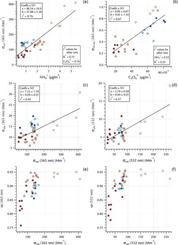
The upwind (Transport/Haze – West) vs. downwind but not to the extent observed during the Stagnant period
(Transport/Haze – East) shift is also evident in the IC anal- (64 % vs. 85 %). For all aerosol components (organics and
yses of these DI extracts (Fig. 4). NO− 3 was up to an order inorganics), concentrations during this period tended to be
of magnitude greater downwind than upwind during Trans- relatively low (Fig. 4).
port/Haze, while peak SO2− 4 nearly doubled, consistent with The measured optical properties exhibited differing rela-
previous reports of local South Korean heterogeneous sec- tionships to the water-soluble aerosol chemical components
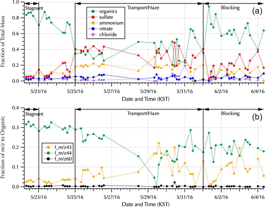
ondary production of these constituents (Jordan et al., 2020). as illustrated in Fig. 5. For example, σext (365 nm) was well
Throughout the cruise, SO2− 4 was generally fully neutral- correlated with the mass concentrations of NH+ 4 and K
+
ized by NH+ 4 , i.e., in the form (NH4 )2 SO4 (Fig. 4). K
+ 2−
but poorly correlated with C2 O4 (0.76, 0.72, and 0.16,
+
was linearly related to NH4 throughout the cruise with an respectively, Fig. 5). The soluble absorption (both DI and
r 2 = 0.78 (Fig. 4). In contrast, C2 O2−
4 measured by IC exhib- MeOH, but only DI shown) was well correlated with C2 O2− 4
ited elevated values both for the Stagnant (and transition) and but poorly correlated NH+ +
4 and K (e.g., σDI-abs (365 nm)
downwind Transport/Haze samples (Fig. 4). Organic aerosol r 2 = 0.67, 0.22, and 0.25, respectively, Fig. 5). This is not
was elevated during the Transport/Haze period (Jordan et al., unexpected as extinction is related to aerosol mass loading
2020), but it did not increase as rapidly or dramatically as and size distributions, while soluble absorption is a func-
SIA, hence the decreased percent contribution to the total tion of soluble aerosol composition. Total aerosol absorp-
Atmos. Meas. Tech., 14, 715–736, 2021 https://doi.org/10.5194/amt-14-715-2021C. E. Jordan et al.: In situ aerosol hyperspectral optical measurements 725
Figure 4. Relationships between SO2− + − + + +
4 and NH4 (a) and NO3 and NH4 (b) in equivalents units and between K and NH4 (c) and C2 O4
2−
+
and K (d) in mass units. Markers are colored by Peterson et al. (2019) meteorological regime with the Transport/Haze – East samples
downwind of South Korea and the Transport/Haze – West samples upwind of South Korea (see Fig. 1) under the prevailing low-level
westerly transport from China during this meteorological regime.
tion was not well correlated with any of the water-soluble tively low during this period, while elevated C2 O2− 4 concen-
aerosol components (as expected, since BC dominates to- trations at this time were independent of K+ (Fig. 4). Both
tal absorption in the atmosphere and is not soluble). How- K+ and C2 O2− 4 have known biomass burning sources and
ever, as shown in the companion paper, peak σabs tended to have been used as tracers for biomass burning (e.g., Park
coincide with peak σext , leading to moderate r 2 values of et al., 2013; Park and Yu, 2016; Szép et al., 2018; Johansen,
∼ 0.5 depending on wavelength (Fig. 5). This is likely a re- et al., 2019). However, they also have other sources that
flection of mass loading, such that when pollutant aerosol can complicate their usage for such a purpose. For exam-
concentrations downwind of South Korea were high, both ple, C2 O2−4 can be formed by aqueous-phase cloud chemi-
scatterers and BC were elevated in the air mass. Single- cal processes (e.g., Huang et al., 2006; Ervens et al., 2011),
scattering albedo clarifies an interesting feature evident in and fine-fraction K+ can arise from fertilizer use (e.g., Szép
σabs ; i.e., the total absorption is sensitive to organic absorbers et al., 2018; Han et al., 2019), fireworks (Hao et al., 2018; ten
at 365 nm (i.e., BrC). There is little difference in ω(365 nm) Brink, et al., 2019), and anthropogenic combustion sources
and ω(532 nm) for the Transport/Haze and Blocking periods; (Jayarathne et al. 2018; Han et al., 2019; Yan et al., 2020)
however, there is a substantial reduction in ω(365 nm) for the such as coal, garbage incineration, and cooking fuels, with
Stagnant (and transition) period samples (Fig. 5). charcoal in particular exhibiting enhanced K+ (Jayarathne
This is a striking observation due to the fact that the Stag- et al. 2018). Levoglucosan has also been used as a biomass
nant period aerosols were dominated by local photochem- burning tracer; however, its relative contribution has been
ically produced SOA. K+ mass concentrations were rela- shown to decrease with smoke plume age (Cubision et al.,
https://doi.org/10.5194/amt-14-715-2021 Atmos. Meas. Tech., 14, 715–736, 2021726 C. E. Jordan et al.: In situ aerosol hyperspectral optical measurements
2−
Figure 5. Relationships between 365 nm σext and NH+ 4 (a), 365 nm σDI-abs and C2 O4 (b), σabs and σext at 365 and 532 nm (c, d, respec-
tively), and ω and σext at 365 and 532 nm (e, f, respectively). Markers are colored by Peterson et al. (2019) meteorological regime (see Figs. 1
and 4).
2011), and recent work indicates that it is short-lived in the 365 nm without any evident indication of biomass burning.
atmosphere such that it is useful for fresh emissions but not However, the Wong et al. (2019) study also reported that ab-
for aged biomass burning aerosol (Wong et al., 2019). Fig- sorbing high-molecular-weight biomass burning aerosol is
ure 3 shows m/z 60 from the nebulized water-soluble ex- relatively stable and much longer lived in the atmosphere
tracts was negligible throughout the campaign. m/z 60 is typ- than low-molecular-weight biomass burning aerosol compo-
ically attributed to the C2 H4 O+
2 fragment from levoglucosan nents such as levoglucosan. The implications of this will be
(Schneider et al., 2006) and is enhanced for the biomass discussed further in Sect. 3.3.
burning organic aerosol PMF factor (Cubison et al., 2011). The differences between ω(365 nm) and ω(532 nm) for
All of these data suggest that during the Stagnant period the absorbing aerosols of the Stagnant period and Trans-
photochemically produced SOA contributed to absorption at port/Haze period show that the elevated C2 O2−
4 and elevated
Atmos. Meas. Tech., 14, 715–736, 2021 https://doi.org/10.5194/amt-14-715-2021C. E. Jordan et al.: In situ aerosol hyperspectral optical measurements 727
σDI-abs do not fully capture differences across these popula- set (e.g., Fig. S4). In Part 1, it was shown that the expanded
tions of absorbing organic aerosols. That is, decreases in ω wavelength range in σext led to smaller values of αext due to
from 532 to 365 nm are small for the Transport/Haze popula- the negative curvature of the spectra. Here, the positive cur-
tion, in contrast to the large decrease for the Stagnant (and vature of the absorption spectra leads to the opposite result,
transition) aerosols. The molecular structures that absorb i.e., larger values of αabs compared to those shown in Part 1
light differ between the two groups such that the photochem- calculated from the visible TAP wavelengths. Hence, when
istry of the Stagnant period appears to have produced molec- comparing Ångström exponents across data sets the role of
ularly different SOA than was produced under the cloudy curvature requires that the wavelength range used to calcu-
hazy conditions of the Transport/Haze period. late α be taken into account. The values may not be directly
It must be emphasized that the chemical contributions dis- comparable as will be discussed further below.
cussed in this section only include aerosol components that The residuals from the second-order polynomial and linear
were soluble in water and hence only represent a portion of fits to each spectra set were binned into 20 bins spanning the
the ambient chemical composition influencing the σext , σabs , full range of differences between each measured spectrum
and σMeOH-abs measurements. σDI-abs contributed only a frac- and fit spectrum (Fig. 6). The range of differences is smaller,
tion to σabs , and σabs values were typically an order of mag- leading to narrower bins for the second-order polynomial fits
nitude smaller than σext . Hence, relationships that may be than the linear fits. The normal distribution around zero of
explored within this data set between chemical composition the second-order polynomial fits shows they provide a better
and optical properties are constrained by these limitations. fit to the data. Following the approach used in the companion
Future work would benefit from concurrent in situ aerosol paper, the additional information that may be gained from the
AMS sampling, as well as size distribution measurements, to coefficients of the second-order fits (a1 and a2 , Eq. 7) than
more fully relate aerosol composition to optical properties. from the Ångström exponent, α (= −b, Eq. 8), provided by
Even so, chromophores may constitute only a small fraction linear fits is examined here.
of the aerosol mass (e.g., Bones et al., 2010). Hence, changes As discussed in detail in Part 1, the coefficients between
in σabs may or may not be tightly coupled to aerosol compo- the two fits are related to each other by the derivatives of
sition measurements. The development of in situ hyperspec- Eqs. (7) and (8), where
tral techniques to measure the optical properties of in situ
d(LN(p(λ))
aerosols, along with the chemical and microphysical proper- α=− = −b = −(a1 + 2a2 (LN(λch )). (9)
ties of those aerosols, is expected to reduce some of the un- dLN(λ)
certainties in assessing the relationships among the full suite Here, the notation λch is used to denote that there is one
of ambient aerosol characteristics. wavelength for which α and (a1 , a2 ) yield equivalent results
for any given spectrum. −2LN(λch ) can be thought of as
3.3 Characterizing spectral shapes with second-order the slope of a line that describes that relationship in (a1 , a2 )
polynomial coefficients space. This is illustrated in Fig. S5, where for each spectra
set λch was calculated from the pair of fits to each spectrum.
While isolating individual wavelengths from the spectral data In the case of σabs , only a very narrow range of values was
can be informative as illustrated in Sect. 3.2, the anticipated found such that λch = 0.47. Using this value in Eq. (9), one
value of these hyperspectral measurements comes from ex- can map the set of parallel α lines into (a1 , a2 ) space using
amining the full spectra. In Part 1 (Jordan et al., 2021) it was the range of values obtained for these coefficients from the
shown that the logarithmically transformed extinction spec- two sets of fits. For any given α, spectra with differing cur-
tra were better fit with a second-order polynomial than a line, vature will map into different pairs of (a1 , a2 ) along that line
due to curvature of the spectra in log space. Similarly, for the (Fig. S5). A plot of the individual α values obtained from
filter spectra sets second-order polynomials, the σabs set (Fig. 7) shows those points are aligned accord-
ing to the map in Fig. S5. Note that the color bars for α used
LN(p(λ)) = a0 + a1 LN(λ) + a2 (LN(λ))2 (7)
in Fig. 7 match those in Fig. S5 (right panels). For σabs , the
yielded better fits to the measured spectra than linear fits (i.e., range of α is 1.08 to 2.80. These are larger values than the
representing a power law), range shown in Part 1 from the visible wavelength TAP data
where αabs ∼ 0.5–1 (Jordan et al., 2021). As noted above,
LN(p(λ)) = a + bLN(λ), (8) positive curvature and a wavelength range extending further
into the UV leads to the higher αabs values here. Previous
of the spectra as shown by the improvement in the fit residu- studies have used αabs to distinguish absorbing aerosol com-
als (Fig. 6). An example set of spectra (Fig. S4) is provided position (e.g., αabs = 1, fresh urban-industrial BC, ≥ 2, desert
in the Supplement to illustrate the difference in the residu- dust, with intermediate values indicative of biomass burn-
als from these two fits. Note that all three absorption spec- ing aerosols; Russell et al., 2010). However, Schuster et al.
tra tended to exhibit positive curvature in contrast to extinc- (2016) caution that mixing state and size distribution play a
tion spectra that are all negative for the filter mean spectra role in αabs along with composition.
https://doi.org/10.5194/amt-14-715-2021 Atmos. Meas. Tech., 14, 715–736, 2021You can also read