WHO 2016 subtyping and automated segmentation of glioma using multi-task deep learning
←
→
Page content transcription
If your browser does not render page correctly, please read the page content below
WHO 2016 subtyping and automated
                                          segmentation of glioma using multi-task
                                                      deep learning
arXiv:2010.04425v1 [eess.IV] 9 Oct 2020

                                            Sebastian R. van der Voort1,† , Fatih Incekara2,3,† , Maarten MJ
                                             Wijnenga4 , Georgios Kapsas2 , Renske Gahrmann2 , Joost W
                                          Schouten3 , Rishi Nandoe Tewarie5 , Geert J Lycklama6 , Philip C
                                          De Witt Hamer7 , Roelant S Eijgelaar7 , Pim J French4 , Hendrikus
                                           J Dubbink8 , Arnaud JPE Vincent3 , Wiro J Niessen1,9 , Martin J
                                               van den Bent4 , Marion Smits2,†† , and Stefan Klein1,††,*
                                          1
                                            Biomedical Imaging Group Rotterdam, Department of Radiology
                                             and Nuclear Medicine, Erasmus MC University Medical Centre
                                                         Rotterdam, Rotterdam, the Netherlands
                                             2
                                               Department of Radiology and Nuclear Medicine, Erasmus MC
                                          University Medical Centre Rotterdam, Rotterdam, the Netherlands
                                          3
                                            Department of Neurosurgery, Brain Tumor Center, Erasmus MC
                                          University Medical Centre Rotterdam, Rotterdam, the Netherlands
                                             4
                                               Department of Neurology, Brain Tumor Center, Erasmus MC
                                                      Cancer Institute, Rotterdam, the Netherlands
                                             5
                                               Department of Neurosurgery, Haaglanden Medical Center, the
                                                                  Hague, the Netherlands
                                               6
                                                 Department of Radiology, Haaglanden Medical Center, the
                                                                  Hague, the Netherlands
                                           8
                                             Department of Pathology, Brain Tumor Center at Erasmus MC
                                                      Cancer Institute, Rotterdam, the Netherlands
                                          9
                                            Imaging Physics, Faculty of Applied Sciences, Delft University of
                                                            Technology, Delft, the Netherlands
                                           7
                                             Department of Neurosurgery, Cancer Center Amsterdam, Brain
                                               Tumor Center, Amsterdam UMC, Amsterdam, Netherlands
                                                            †
                                                              These authors contributed equally
                                                           ††
                                                              These authors contributed equally
                                                      *
                                                        Corresponding author; s.klein@erasmusmc.nl

                                                                           1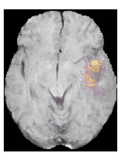
Abstract
          Accurate characterization of glioma is crucial for clinical decision mak-
      ing. A delineation of the tumor is also desirable in the initial decision
      stages but is a time-consuming task. Leveraging the latest GPU capabil-
      ities, we developed a single multi-task convolutional neural network that
      uses the full 3D, structural, pre-operative MRI scans to can predict the
      IDH mutation status, the 1p/19q co-deletion status, and the grade of a tu-
      mor, while simultaneously segmenting the tumor. We trained our method
      using the largest, most diverse patient cohort to date containing 1508
      glioma patients from 16 institutes. We tested our method on an indepen-
      dent dataset of 240 patients from 13 different institutes, and achieved an
      IDH-AUC of 0.90, 1p/19q-AUC of 0.85, grade-AUC of 0.81, and a mean
      whole tumor DICE score of 0.84. Thus, our method non-invasively pre-
      dicts multiple, clinically relevant parameters and generalizes well to the
      broader clinical population.

1    Introduction
Glioma is the most common primary brain tumor and is one of the deadliest
forms of cancer [1]. Differences in survival and treatment response of glioma are
attributed to their genetic and histological features, specifically the isocitrate
dehydrogenase (IDH) mutation status, the 1p/19q co-deletion status and the
tumor grade [2, 3]. Therefore, in 2016 the World Health Organization (WHO)
updated its brain tumor classification, categorizing glioma based on these ge-
netic and histological features [4]. In current clinical practice, these features are
determined from tumor tissue. While this is not an issue in patients in whom
the tumor can be resected, this is problematic when resection can not safely
be performed. In these instances, surgical biopsy is performed with the sole
purpose of obtaining tissue for diagnosis, which, although relatively safe, is not
without risk [5, 6]. Therefore, there has been an increasing interest in comple-
mentary non-invasive alternatives that can provide the genetic and histological
information used in the WHO 2016 categorization [7, 8].
    Magnetic resonance imaging (MRI) has been proposed as a possible candi-
date because of its non-invasive nature and its current place in routine clinical
care [9]. Research has shown that certain MRI features, such as the tumor het-
erogeneity, correlate with the genetic and histological features of glioma [10, 11].
This notion has popularized, in addition to already popular applications such
as tumor segmentation, the use of machine learning methods for the prediction
of genetic and histological features, known as radiomics [12, 13, 14]. Although
a plethora of such methods now exist, they have found little translation to the
clinic [12].
    An often discussed challenge for the adoption of machine learning methods
in clinical practice is the lack of standardization, resulting in heterogeneity of
patient populations, imaging protocols, and scan quality [15, 16]. Since machine
learning methods are prone to overfitting, this heterogeneity questions the va-
lidity of such methods in a broader patient population [16]. Furthermore, it has

                                           2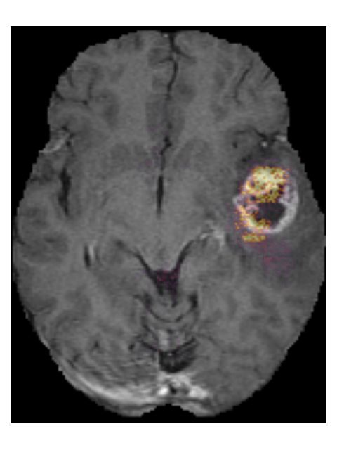
been noted that most current research concerns narrow task-specific methods
that lack the context between different related tasks, which might restrict the
performance of these methods [17].
    An important technical limitation when using deep learning methods is the
limited GPU memory, which restricts the size of models that can be trained
[18]. This is a problem especially for clinical data, which is often 3D, requiring
even more memory than the commonly used 2D networks. This further limits
the size of these models resulting in shallower models, and the use of patches of
a scan instead of using the full 3D scan as an input, which limits the amount of
context these methods can extract from the scans.
    Here, we present a new method that addresses the above problems. Our
method consists of a single, multi-task convolutional neural network (CNN)
that can predict the IDH mutation status, the 1p/19q co-deletion status, and
the grade (grade II/III/IV) of a tumor, while also simultaneously segmenting the
tumor, see Figure 1. To the best of our knowledge, this is the first method that
provides all of this information at the same time, allowing clinical experts to de-
rive the WHO category from the individually predicted genetic and histological
features, while also allowing them to consider or disregard specific predictions
as they deem fit. Exploiting the capabilities of the latest GPUs, optimizing our
implementation to reduce the memory footprint, and using distributed multi-
GPU training, we were able to train a model that uses the full 3D scan as an
input. We trained our method using the largest, most diverse patient cohort
to date, with 1508 patients included from 16 different institutes. To ensure
the broad applicability of our method, we used minimal inclusion criteria, only
requiring the four most commonly used MRI sequences: pre- and post-contrast
T1-weighted (T1w), T2-weighted (T2w), and T2-weighted fluid attenuated in-
version recovery (T2w-FLAIR) [19, 20]. No constraints were placed on the
patients’ clinical characteristics, such as the tumor grade, or the radiological
characteristics of scans, such as the scan quality. In this way, our method could
capture the heterogeneity that is naturally present in clinical data. We tested
our method on an independent dataset of 240 patients from 13 different insti-
tutes, to evaluate the true generalizability of our method. Our results show that
we can predict multiple clinical features of glioma from MRI scans in a diverse
patient population.

                                        3
Preprocessed      Convolutional
     MRI scans                                               Segmentation
                        scans          neural network

                                                              WHO 2016
                                                             categorization
                                                                IDH status
                                                           Wildtype         Mutated

                                                              1p/19q status

                                                             Intact    Co-deleted

                                                                    Grade
                                                               II     III     IV

Figure 1: Overview of our method. Pre-, and post-contrast T1w, T2w and T2w-
FLAIR scans are used as an input. The scans are registered to an atlas, bias
field corrected, skull stripped, and normalized before being passed through our
convolutional neural network. One branch of the network segments the tumor,
while at the same time the features are combined to predict the IDH status,
1p/19q status, and grade of the tumor.

                                      4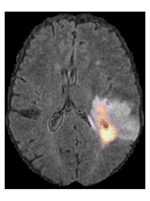
2     Results
2.1    Patient characteristics
We included a total of 1748 patients in our study, 1508 as a train set and
240 as an independent test set. The patients in the train set originated from
nine different data collections and 16 different institutes, and the test set was
collected from two different data collections and 13 different institutes. Table 1
provides a full overview of the patient characteristics in the train and test set,
and Figure 2 shows the inclusion flowchart and the distribution of the patients
over the different data collections in the train set and test set.

         Table 1: Patient characteristics for the train set and test set.

                                            Train set           Test set
                                              N     %            N     %
        Patients                            1508               240
        IDH status
          Mutated                            226   15.0         88   36.7
          Wildtype                           440   29.2        129   53.7
          Unknown                            842   55.8         23    9.6
        1p/19q co-deletion status
          Co-deleted                         103    6.8         26   10.8
          Intact                             337   22.4        207   86.3
          Unknown                           1068   70.8          7    2.9
        Grade
          II                                230    15.3         47   19.6
          III                               114     7.6         59   24.6
          IV                                830    55.0        132   55.0
          Unknown                           334    22.1          2    0.8
        WHO 2016 categorization
          Oligodendroglioma                  96     6.4         26   10.8
          Astrocytoma, IDH wildtype          31     2.1         22    9.2
          Astrocytoma, IDH mutated           98     6.4         57   23.7
          GBM, IDH wildtype                 331    21.9        106   44.2
          GBM, IDH mutated                   16     1.1          5    2.1
          Unknown                           936    62.1         24   10.0
        Segmentation
          Manual                             716   47.5        240    100
          Automatic                          792   52.5          0      0
IDH: isocitrate dehydrogenase, WHO: World Health Organization, GBM:
glioblastoma

                                        5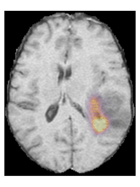
Patient screening
Train set
2181 Glioma patients

1241   Erasmus MC
 491   Haaglanden Medical Center
 168   BraTS
 130   REMBRANDT
  66   CPTAC-GBM
  39   Ivy GAP
  20   Amsterdam UMC                           Patient exclusion
  20   Brain-Tumor-Progression
   6   University Medical Center Utrecht       Train set
                                               673 No pre-operative
Test set                                            pre-, or post-contrast T1w,
 461 Glioma patients                                T2w or T2w-FLAIR

 199 TCGA-LGG                                  425   Erasmus MC
 262 TCGA-GBM                                  212   Haaglanden Medical Center
                                                 0   BraTS
                                                21   REMBRANDT
                                                15   CPTAC-GBM
                                                 0   Ivy GAP
                                                 0   Amsterdam UMC
                                                 0   Brain-Tumor-Progression
                                                 0   University Medical Center Utrecht
Patient inclusion
                                               Test set
Train set                                      221 No pre-operative
1508 Patients in train set                           pre-, or post-contrast T1w,
                                                     T2w or T2w-FLAIR
 816   Erasmus MC
 279   Haaglanden Medical Center               92  TCGA-LGG
 168   BraTS                                   129 TCGA-GBM
 109   REMBRANDT
  51   CPTAC-GBM
  39   Ivy GAP
  20   Amsterdam UMC
  20   Brain-Tumor-Progression
   6   University Medical Center Utrecht

Test set
 240 Patients in test set

 107 TCGA-LGG
 133 TCGA-GBM

            Figure 2: Inclusion flowchart of the train set and test set.

                                           6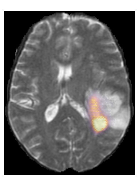
2.2 Algorithm performance
We used 15% of the train set as a validation set and selected the model pa-
rameters that achieved the best performance on this validation set, where the
model achieved an area under receiver operating characteristic curve (AUC) of
0.88 for the IDH mutation status prediction, an AUC of 0.76 for the 1p/19q
co-deletion prediction, an AUC of 0.75 for the grade prediction, and a mean
segmentation DICE score of 0.81. The selected model parameters are shown in
Appendix F. We then trained a model using these parameters and the full train
set, and evaluated it on the independent test set.
For the genetic and histological feature predictions, we achieved an AUC of
0.90 for the IDH mutation status prediction, an AUC of 0.85 for the 1p/19q
co-deletion prediction, and an AUC of 0.81 for the grade prediction, in the
test set. The full results are shown in Table 2, with the corresponding receiver
operating characteristic (ROC)-curves in Figure 3. Table 2 also shows the results
in (clinically relevant) subgroups of patients. This shows that we achieved an
IDH-AUC of 0.81 in low grade glioma (LGG) (grade II/III), an IDH-AUC of
0.64 in high grade glioma (HGG) (grade IV), and a 1p/19q-AUC of 0.73 in LGG.
When only predicting LGG vs. HGG instead of predicting the individual grades,
we achieved an AUC of 0.91. In Appendix A we provide confusion matrices for
the IDH, 1p/19q, and grade predictions, as well as a confusion matrix for the
final WHO 2016 subtype, which shows that only one patient was predicted as
a non-existing WHO 2016 subtype. In Appendix C we provide the individual
predictions and ground truth labels for all patients in the test set to allow for
the calculation of additional metrics.
For the automatic segmentation, we achieved a mean DICE score of 0.84, a
mean Hausdorff distance of 18.9 mm, and a mean volumetric similarity coeffi-
cient of 0.90. Figure 4 shows boxplots of the DICE scores, Hausdorff distances,
and volumetric similarity coefficients for the different patients in the test set. In
Appendix B we show five patients that were randomly selected from both the
TCGA-LGG and TCGA-GBM data collections, to demonstrate the automatic
segmentations made by our method.
2.3 Model interpretability
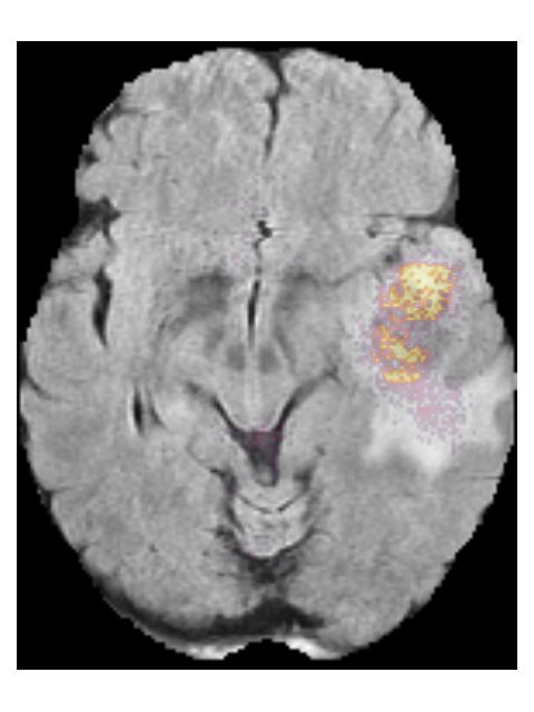
To provide insight into the behavior of our model we created saliency maps,
which show which parts of the scans contributed the most to the prediction.
These saliency maps are shown in Figure 5 for two example patients from the
test set. It can be seen that for the LGG the network focused on a bright rim in
the T2w-FLAIR scan, whereas for the HGG it focused on the enhancement in the
post-contrast T1w scan. To aid further interpretation, we provide visualizations
of selected filter outputs in the network in Appendix D, which also show that
the network focuses on the tumor, and these filters seem to recognize specific
imaging features such as the contrast enhancement and T2w-FLAIR brightness.
7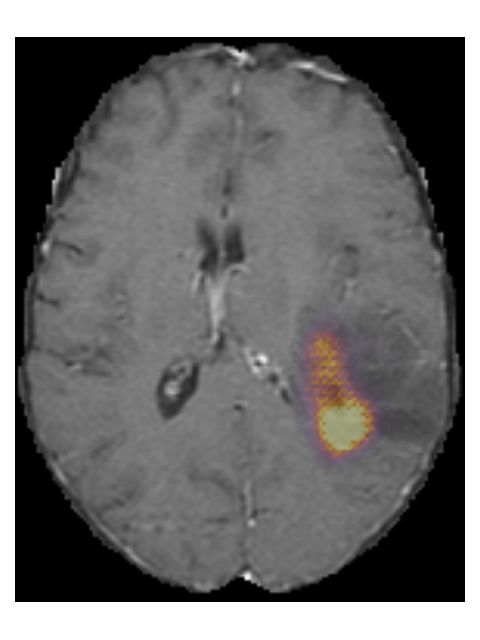
Table 2: Evaluation results of the final model on the test set.

 Patient
             Task                    AUC         Accuracy      Sensitivity     Specificity
  group

 All         IDH                      0.90          0.84          0.72            0.93
             1p/19q                   0.85          0.89          0.39            0.95
             Grade (II/III/IV)        0.81          0.71          N/A             N/A
             Grade II                 0.91          0.86          0.75            0.89
             Grade III                0.69          0.75          0.17            0.94
             Grade IV                 0.91          0.82          0.95            0.66
             LGG vs HGG               0.91          0.84          0.72            0.93

 LGG         IDH                      0.81          0.74          0.73            0.77
             1p/19q                   0.73          0.76          0.39            0.89

 HGG         IDH                      0.64          0.94          0.40            0.96
Abbreviations: AUC: area under receiver operating characteristic curve, IDH:
isocitrate dehydrogenase, LGG: low grade glioma, HGG: high grade glioma

Figure 3: Receiver operating characteristic (ROC)-curves of the genetic and
histological features, evaluated on the test set. The crosses indicate the location
of the decision threshold for the reported accuracy, sensitivity, and specificity.

                                         8
Figure 4: DICE scores, Hausdorff distances, and volumetric similarity coeffi-
cients for all patients in the test set. The DICE score is a measure of the
overlap between the ground truth and predicted segmentation (where 1 indi-
cates perfect overlap). The Hausdorff distance is a measure of the agreement
between the boundaries of the ground truth and predicted segmentation (lower
is better). The volumetric similarity coefficient is a measure of the agreement
in volume (where 1 indicates perfect agreement).
9Pre-contrast T1w Post-contrast T1w T2w T2w-FLAIR
(a) Saliency maps of a low grade glioma patient (TCGA-DU-6400). This is an IDH mu-
tated, 1p/19q co-deleted, grade II tumor. The network focuses on a rim of brightness
in the T2w-FLAIR scan.
Pre-contrast T1w Post-contrast T1w T2w T2w-FLAIR
(b) Saliency maps of a high grade glioma patient (TCGA-06-0238). This is an IDH
wildtype, grade IV tumor. The network focuses on enhancing spots around the necrosis
on the post-contrast T1w scan.
Figure 5: Saliency maps of two patients from the test set, showing areas that
are relevant for the prediction.
102.4 Model robustness
By not excluding scans from our train set based on radiological characteristics,
we were able to make our model robust to low scan quality, as can be seen in an
example from the test set in Figure 6. Even though this example scan contained
imaging artifacts, our method was able to properly segment the tumor (DICE
score of 0.87), and correctly predict the tumor as an IDH wildtype, grade IV
tumor.
Figure 6: Example of a T2w-FLAIR scan containing imaging artifacts, and the
automatic segmentation (red overlay) made by our method. It was correctly
predicted as an IDH wildtype, grade IV glioma. This is patient TCGA-06-5408
from the TCGA-GBM collection.
Finally, we considered two examples of scans that were incorrectly predicted
by our method, see Figure 7. These two examples were chosen because our
network assigned high prediction scores to the wrong classes for these cases.
Figure 7a shows an example of a grade II, IDH mutated, 1p/19q co-deleted
glioma that was predicted as grade IV, IDH wildtype by our method. Our
method’s prediction was most likely caused by the hyperintensities in the post-
contrast T1w scan being interpreted as contrast enhancement. Since these hy-
perintensities are also present in the pre-contrast T1w scan they are most likely
calcifications, and the radiological appearance of this tumor is indicative of an
oligodendroglioma. Figure 7b shows an example of a grade IV, IDH wildtype
glioma that was predicted as a grade III, IDH mutated glioma by our method.
11Pre-contrast T1w Post-contrast T1w T2w T2w-FLAIR
(a) TCGA-DU-6410 from the TCGA-LGG collection. The ground truth histopatho-
logical analysis indicated this glioma was grade II, IDH mutated, 1p/19q co-deleted,
but our method predicted it as a grade IV, IDH wildtype.
Pre-contrast T1w Post-contrast T1w T2w T2w-FLAIR
(b) TCGA-76-7664 from the TCGA-HGG collection. Histopathologically this glioma
was grade IV, IDH wildtype, but our method predicted it as grade III, IDH mutated.
Figure 7: Examples of scans that were incorrectly predicted by our method.
123 Discussion
We have developed a method that can predict the IDH mutation status, 1p/19q
co-deletion status, and grade of glioma, while simultaneously providing the tu-
mor segmentation, based on pre-operative MRI scans. For the genetic and
histological feature predictions, we achieved an AUC of 0.90 for the IDH mu-
tation status prediction, an AUC of 0.85 for the 1p/19q co-deletion prediction,
and an AUC of 0.81 for the grade prediction, in the test set.
In an independent test set, which contained data from 13 different institutes,
we demonstrated that our method predicts these features with good overall per-
formance; we achieved an AUC of 0.90 for the IDH mutation status prediction,
an AUC of 0.85 for the 1p/19q co-deletion prediction, and an AUC of 0.81 for
the grade prediction, and a mean whole tumor DICE score of 0.84. This per-
formance on unseen data that was only used during the final evaluation of the
algorithm, and that was purposefully not used to guide any decisions regarding
the method design, shows the true generalizability of our method. Using the
latest GPU capabilities we were able to train a large model, which uses the
full 3D scan as input. Furthermore, by using the largest, most diverse patient
cohort to date we were able to make our method robust to the heterogeneity
that is naturally present in clinical imaging data, such that it generalizes for
broad application in clinical practice.
By using a multi-task network, our method could learn the context between
different features. For example, IDH wildtype and 1p/19q co-deletion are mu-
tually exclusive [21]. If two separate methods had been used, one to predict the
IDH status and one to predict the 1p/19q co-deletion status, an IDH wildtype
glioma might be predicted to be 1p/19q co-deleted, which does not stroke with
the clinical reality. Since our method learns both of these genetic features si-
multaneously, it correctly learned not to predict 1p/19q co-deletion in tumors
that were IDH wildtype; there was only one patient in which our algorithm pre-
dicted a tumor to be both IDH wildtype and 1p/19q co-deleted. Furthermore,
by predicting the genetic and histological features individually, instead of only
predicting the WHO 2016 category, it is possible to adopt updated guidelines
such as cIMPACT-NOW, future-proofing our method [22].
Some previous studies also used multi-task networks to predict the genetic
and histological features of glioma [23, 24, 25]. Tang et al. [23] used a multi-task
network that predicts multiple genetic features, as well as the overall survival
of glioblastoma. Since their method only works for glioblastoma patients, the
tumor grade must be known in advance, complicating the use of their method
in the pre-operative setting when tumor grade is not yet known. Furthermore,
their method requires a tumor segmentation prior to application of their method,
which is a time-consuming, expert task. In a study by Xue et al. [24], a multi-
task network was used, with a structure similar to the one proposed in this
paper, to segment the tumor and predict the grade (LGG or HGG) and IDH
mutation status. However, they do not predict the 1p/19q co-deletion status
needed for the WHO 2016 categorization. Lastly, Decuyper et al. [25] used
a multi-task network that predicts the IDH mutation and 1p/19q co-deletion
13status, and the tumor grade (LGG or HGG). Their method requires a tumor
segmentation as input, which they obtain from a U-Net that is applied earlier
in their pipeline; thus, their method requires two networks instead of the single
network we use in our method. These differences aside, the most important
limitation of each of these studies is the lack of an independent test set for
evaluating their results. It is now considered essential that an independent test
set is used, to prevent an overly optimistic estimate of a method’s performance
[15, 26, 27, 28]. Thus, our study improves on this previous work by providing
a single network that combines the different tasks, being trained on a more
extensive and diverse dataset, not requiring a tumor segmentation as an in-
put, providing all information needed for the WHO 2016 categorization, and,
crucially, by being evaluated in an independent test set.
An important genetic feature that is not predicted by our method is the
O6 -methylguanine-methyltransferase (MGMT) methylation status. Although
the MGMT methylation status is not part of the WHO 2016 categorization,
it is part of clinical management guidelines and is an important prognostic
marker in glioblastoma [4]. In the initial stages of this study, we attempted
to predict the MGMT methylation status; however, the performance of this
prediction was poor. Furthermore, the methylation cutoff level, which is used
to determine whether a tumor is MGMT methylated, shows a wide variety
between institutes, leading to inconsistent results [29]. We therefore opted not to
include the MGMT prediction at all, rather than to provide a poor prediction of
an unsharply defined parameter. Although some methods attempted to predict
the MGMT status, with varying degrees of success, there is still an ongoing
discussion on the validity of MR imaging features of the MGMT status [23, 30,
31, 32, 33].
Our method shows good overall performance, but there are noticeable per-
formance differences between tumor categories. For example, when our method
predicts a tumor as an IDH wildtype glioblastoma, it is correct almost all of the
time. On the other hand, it has some difficulty differentiating IDH mutated,
1p/19q co-deleted low-grade glioma from other low-grade glioma. The sensitiv-
ity for the prediction of grade III glioma was low, which might be caused by
the lack of a central pathology review. Because of this, there were differences in
molecular testing and histological analysis, and it is known that distinguishing
between grade II and grade III has a poor observer reliability [34]. Although
our method can be relevant for certain subgroups, our method’s performance
still needs to be improved to ensure relevancy for the full patient population.
In future work, we aim to increase the performance of our method by includ-
ing perfusion-weighted imaging (PWI) and diffusion-weighted imaging (DWI)
since there has been an increasing amount of evidence that these physiologi-
cal imaging modalities contain additional information that correlates with the
tumor’s genetic status and aggressiveness [35, 36]. They were not included in
this study since PWI and, to a lesser extent, DWI are not as ingrained in the
clinical imaging routine as the structural scans used in this work [19, 20]. Thus,
including these modalities would limit our method’s clinical applicability and
substantially reduce the number of patients in the train and test set. However,
14PWI and DWI are increasingly becoming more commonplace, which will allow
including these in future research and which might improve performance.
In conclusion, we have developed a non-invasive method that can predict the
IDH mutation status, 1p/19q co-deletion status, and grade of glioma, while at
the same time segmenting the tumor, based on pre-operative MRI scans with
high overall performance. Although the performance of our method might need
to be improved before it will find widespread clinical acceptance, we believe that
this research is an important step forward in the field of radiomics. Predict-
ing multiple clinical features simultaneously steps away from the conventional
single-task methods and is more in line with the clinical practice where multiple
clinical features are considered simultaneously and may even be related. Fur-
thermore, by not limiting the patient population used to develop our method to
a selection based on clinical or radiological characteristics, we alleviate the need
for a priori (expert) knowledge, which may not always be available. Although
steps still have to be taken before radiomics will find its way into the clinic,
especially in terms of performance, our work provides a crucial step forward by
resolving some of the hurdles of clinical implementation now, and paving the
way for a full transition in the future.
4 Methods
4.1 Patient population
The train set was collected from four in-house datasets and five publicly avail-
able datasets. In-house datasets were collected from four different institutes:
Erasmus MC (EMC), Haaglanden Medical Center (HMC), Amsterdam UMC
(AUMC) [37], and University Medical Center Utrecht (UMCU). Four of the five
public datasets were collected from The Cancer Imaging Archive (TCIA) [38]:
the Repository of Molecular Brain Neoplasia Data (REMBRANDT) collection
[39], the Clinical Proteomic Tumor Analysis Consortium Glioblastoma Multi-
forme (CPTAC-GBM) collection [40], the Ivy Glioblastoma Atlas Project (Ivy
GAP) collection [41, 42], and the Brain-Tumor-Progression collection [43]. The
fifth dataset was the 2019 Brain Tumor Segmentation challenge (BraTS) chal-
lenge dataset [44, 45, 46], from which we excluded the patients that were also
available in the TCGA-LGG and TCGA-GBM collections [47, 48].
For the internal datasets from the EMC and the HMC, manual segmentations
were available, which were made by four different clinical experts. For patients
where segmentations from more than one observer were available, we randomly
picked one of the segmentations to use in the train set. The segmentations
from the AUMC data were made by a single observer of the study by Visser
et al. [37]. From the public datasets, only the BraTS dataset and the Brain-
Tumor-Progression dataset provided manual segmentations. Segmentations of
the BraTS dataset, as provided in the 2019 training and validation set were
used. For the Brain-Tumor-Progression dataset, the segmentations as provided
in the TCIA data collection were used.
15Patients were included if pre-operative pre- and post-contrast T1w, T2w,
and T2w-FLAIR scans were available; no further inclusion criteria were set.
For example, patients were not excluded based on the radiological characteristics
of the scan, such as low imaging quality or imaging artifacts, or the glioma’s
clinical characteristics such as the grade. If multiple scans of the same contrast
type were available in a single scan session (e.g., multiple T2w scans), the scan
upon which the segmentation was made was selected. If no segmentation was
available, or the segmentation was not made based on that scan contrast, the
scan with the highest axial resolution was used, where a 3D acquisition was
preferred over a 2D acquisition.
For the in-house data, genetic and histological data were available for the
EMC, HMC, and UMCU dataset, which were obtained from analysis of tumor
tissue after biopsy or resection. Genetic and histological data of the public
datasets were also available for the REMBRANDT, CPTAC-GBM, and Ivy
GAP collections. Data for the REMBRANDT and CPTAC-GBM collections
was collected from the clinical data available at the TCIA [40, 39]. For the
Ivy GAP collection, the genetic and histological data were obtained from the
Swedish Institute at https://ivygap.swedish.org/home.
As a test set we used the TCGA-LGG and TCGA-GBM collections from the
TCIA [47, 48]. Genetic and histological labels were obtained from the clinical
data available at the TCIA. Segmentations were used as available from the
TCIA, based on the 2018 BraTS challenge [45, 49, 50]. The inclusion criteria
for the patients included in the BraTS challenge were the same as our inclusion
criteria: the presence of a pre-operative pre- and post-contrast T1w, T2w, and
T2w-FLAIR scan. Thus, patients from the TCGA-LGG and TCGA-GBM were
included if a segmentation from the BraTS challenge was available. However,
for three patients, we found that although they did have manual segmentations,
they did not meet our inclusion requirements: TCGA-08-0509 and TCGA-08-
0510 from TCGA-GBM because they did not have a pre-contrast T1w scan and
TCGA-FG-7634 from TCGA-LGG because there was no post-contrast T1w
scan.
4.2 Automatic segmentation in the train set
To present our method with a large diversity in scans, we wanted to include as
many patients in the train set as possible from the different datasets. Therefore,
we performed automatic segmentation in patients that did not have manual
segmentations. To this end, we used an initial version of our network (presented
in Section 4.4), without the additional layers that were needed for the prediction
of the genetic and histological features. This network was initially trained using
all patients in the train set for whom a manual segmentation was available,
and this trained network was then applied to all patients for which a manual
segmentation was not available. The resulting automatic segmentations were
inspected, and if their quality was acceptable, they were added to the train
set. The network was then trained again, using this increased dataset, and was
applied to scans that did not yet have a segmentation of acceptable quality.
16This process was repeated until an acceptable segmentation was available for
all patients, which constituted our final, complete train set.
4.3 Pre-processing
For all datasets, except for the BraTS dataset for which the scans were already
provided in NIfTI format, the scans were converted from DICOM format to
NIfTI format using dcm2niix version v1.0.20190410 [51]. We then registered
all scans to the MNI152 T1w and T2w atlases, version ICBM 2009a, which
had a resolution of 1x1x1 mm3 and a size of 197x233x189 voxels [52, 53]. The
scans were affinely registered using Elastix 5.0 [54, 55]. The pre- and post-
contrast T1w scans were registered to the T1w atlas; the T2w and T2w-FLAIR
scans were registered to the T2w atlas. When a manual segmentation was
available for patients from the in-house datasets, the registration parameters
that resulted from registering the scan used during the segmentation were used
to transform the segmentation to the atlas. In the case of the public datasets,
we used the registration parameters of the T2w-FLAIR scans to transform the
segmentations.
After the registration, all scans were N4 bias field corrected using SimpleITK
version 1.2.4 [56]. A brain mask was made for the atlas using HD-BET, both for
the T1w atlas and the T2w atlas [57]. This brain mask was used to skull strip
all registered scans and crop them to a bounding box around the brain mask,
reducing the amount of background present in the scans, resulting in a scan size
of 152x182x145 voxels. Subsequently, the scans were normalized such that for
each scan, the average image intensity was 0, and the standard deviation of the
image intensity was 1 within the brain mask. Finally, the background outside
the brain mask was set to the minimum intensity value within the brain mask.
Since the segmentation could sometimes be rugged at the edges after regis-
tration, especially when the segmentations were initially made on low-resolution
scans, we smoothed the segmentation using a 3x3x3 median filter (this was only
done in the train set). For segmentations that contained more than one la-
bel, e.g., when the tumor necrosis and enhancement were separately segmented,
all labels were collapsed into a single label to obtain a single segmentation of
the whole tumor. The genetic and histological labels and the segmentations of
each patient were one-hot encoded. The four scans, ground truth labels, and
segmentation of each patient were then used as the input to the network.
4.4 Model
We based the architecture of our model on the U-Net architecture, with some
adaptations made to allow for a full 3D input and the auxiliary tasks [58]. Our
network architecture, which we have named PrognosAIs Structure-Net, or PS-
Net for short, can be seen in Figure 8.
To use the full 3D scan as an input to the network, we replaced the first
pooling layer that is usually present in the U-Net with a strided convolution,
with a kernel size of 9x9x9 and a stride of 3x3x3. In the upsampling branch of
17145x182x152
Segmentation
32 32 2
49x61x51
32 64 64 32
25x31x26
128 128 64
13x16x13
256 256 128
7x8x7
512 256
IDH
512 2
1p/19q
1472 512 2
Grade
512 3
Batch normalization Concatenation Convolution & ReLU Convolution & Softmax
3x3x3 1x1x1
(De)convolution & ReLU Dense & ReLU Dense & Softmax Dropout
9x9x9
stride 3x3x3
Max pooling Up-convolution & ReLU Global max
2x2x2 2x2x2 pooling
Figure 8: Overview of the PrognosAIs Structure-Net (PS-Net) architecture used
for our model. The numbers below the different layers indicate the number of
filters, dense units or features at that layer. We have also indicated the feature
map size at the different depths of the network.
the network, the last up-convolution is replaced by a deconvolution, with the
same kernel size and stride.
At each depth of the network, we have added global max-pooling layers
directly after the dropout layer, to obtain imaging features that can be used to
predict the genetic and histological features. We chose global pooling layers as
they do not introduce any additional parameters that need to be trained, thus
keeping the memory required by our model manageable. The features from the
different depths of the network were concatenated and fed into three different
dense layers, one for each of the genetic and histological outputs.
l2 kernel regularization was used in all convolutional layers, except for the
last convolutional layer used for the output of the segmentation. In total this
model contained 27,042,473 trainable an 2,944 non-trainable parameters.
184.5 Model training
Training of the model was done on eight NVidia RTX2080Ti’s with 11GB of
memory, using TensorFlow 2.2.0 [59]. To be able to use the full 3D scan as
input to the network, without running into memory issues, we had to optimize
the memory efficiency of the model training. Most importantly, we used mixed-
precision training, which means that most of the variables of the model (such as
the weights) were stored in float16, which requires half the memory of float32,
which is typically used to store these variables [60]. Only the last softmax
activation layers of each output were stored as float32. We also stored our
pre-processed scans as float16 to further reduce memory usage.
However, even with these settings, we could not use a batch size larger than
1. It is known that a larger batch size is preferable, as it increases the stability
of the gradient updates and allows for a better estimation of the normalization
parameters in batch normalization layers [61]. Therefore, we distributed the
training over the eight GPUs, using the NCCL AllReduce algorithm, which
combines the gradients calculated on each GPU before calculating the update
to the model parameters [62]. We also used synchronized batch normalization
layers, which synchronize the updates of their parameters over the distributed
models. In this way, our model had a virtual batch size of eight for the gradient
updates and the batch normalization layers parameters.
To provide more samples to the algorithm and prevent potential overtrain-
ing, we applied four types of data augmentation during training: cropping,
rotation, brightness shifts, and contrast shifts. Each augmentation was applied
with a certain augmentation probability, which determined the probability of
that augmentation type being applied to a specific sample. When an image was
cropped, a random number of voxels between 0 and 20 was cropped from each
dimension, and filled with zeros. For the random rotation, an angle between
−30◦ and 30◦ degrees was selected from a uniform distribution for each dimen-
sion. The brightness shift was applied with a delta uniformly drawn between
0 and 0.2, and the contrast shift factor was randomly drawn between 0.85 and
1.15. We also introduced an augmentation factor, which determines how often
each sample was parsed as an input sample during a single epoch, where each
time it could be augmented differently.
For the IDH, 1p/19q, and grade output, we used a masked categorical cross-
entropy loss, and for the segmentation we used a DICE loss, see Appendix E for
details. We used AdamW as an optimizer, which has shown improved general-
ization performance over Adam by introducing the weight decay parameter as a
separate parameter from the learning rate [63]. The learning rate was automat-
ically reduced by a factor of 0.25 if the loss did not improve during the last five
epochs, with a minimum learning rate of 1 · 10−11 . The model could train for a
maximum of 150 epochs, and training was stopped early if the average loss over
the last five epochs did not improve. Once the model was finished training, the
weights from the epoch with the lowest loss were restored.
194.6 Hyperparameter tuning
Hyperparameters involved in the training of the model needed to be tuned to
achieve the best performance. We tuned a total of six hyper parameters: the l2-
norm, the dropout rate, the augmentation factor, the augmentation probability,
the optimizer’s initial learning rate and the optimizer’s weight decay. A full
overview of the trained parameters and the values tested for the different settings
is presented in Appendix F.
To tune these hyperparameters, we split the train set into a hyperparameter
training set (85%/1282 patients of the full train data) and a hyperparameter
validation set (15%/226 patients of the full train data). Models were trained for
different hyperparameter settings via an exhaustive search using the hyperpa-
rameter train set, and then evaluated on the hyperparameter validation set. No
data augmentation was applied to the hyperparameter validation to ensure that
results between trained models were comparable. The hyperparameters that led
to the lowest overall loss in the hyperparameter validation set were chosen as
the optimal hyperparameters. We trained the final model using these optimal
hyperparameters and the full train set.
4.7 Post-processing
The predictions of the network were post-processed to obtain the final predicted
labels and segmentations for the samples. Since softmax activations were used
for the genetic and histological outputs, a prediction between 0 and 1 was out-
putted for each class, where the individual predictions summed to 1. The final
predicted label was then considered as the class with the highest prediction score.
For the prediction of LGG (grade II/III) vs. HGG (grade IV), the prediction
scores of grade II and grade III were combined to obtain the prediction score
for LGG, the prediction score of grade IV was used as the prediction score for
HGG. If a segmentation contained multiple unconnected components, we only
retained the largest component to obtain a single whole tumor segmentation.
4.8 Model evaluation
The performance of the final trained model was evaluated on the independent
test set, comparing the predicted labels with the ground truth labels. For the
genetic and histological features, we evaluated the AUC, the accuracy, the sen-
sitivity, and the specificity using scikit-learn version 0.23.1, for details see Ap-
pendix G [64]. We evaluated these metrics on the full test set and in subcate-
gories relevant to the WHO 2016 guidelines. We evaluated the IDH performance
separately in the LGG (grade II/III) and HGG (grade IV) subgroups, the 1p/19q
performance in LGG, and we also evaluated the performance of distinguishing
between LGG and HGG instead of predicting the individual grades.
To evaluate the performance of the segmentation, we calculated the DICE
scores, Hausdorff distances, and volumetric similarity coefficient comparing the
automatic segmentation of our method and the manual ground truth segmen-
20tations for all patients in the test set. These metrics were calculated using
the EvaluateSegmentation toolbox, version 2017.04.25 [65], for details see Ap-
pendix G.
To prevent an overly optimistic estimation of our model’s predictive value,
we only evaluated our model on the test set once all hyperparameters were
chosen, and the final model was trained. In this way, the performance in the
test set did not influence decisions made during the development of the model,
preventing possible overfitting by fine-tuning to the test set.
To gain insight into the model, we made saliency maps that show which
parts of the scan contribute the most to the prediction of the CNN [66]. Saliency
maps were made using tf-keras-vis 0.5.2, changing the activation function of all
output layers from softmax to linear activations, using SmoothGrad to reduce
the noisiness of the saliency maps [66].
Another way to gain insight into the network’s behavior is to visualize the
filter outputs of the convolutional layers, as they can give some idea as to what
operations the network applies to the scans. We visualized the filter outputs of
the last convolutional layers in the downsample and upsample path at the first
depth (at an image size of 49x61x51) of our network. These filter outputs were
visualized by passing a sample through the network and showing the convolu-
tional layers’ outputs, replacing the ReLU activation with linear activations.
4.9 Data availability
An overview of the patients included from the public datasets used in the train-
ing and testing of the algorithm, and their ground truth label is available in
Appendix H. The data from the public datasets are available in TCIA un-
der DOIs: 10.7937/K9/TCIA.2015.588OZUZB, 10.7937/k9/tcia.2018.3rje41q1,
10.7937/K9/TCIA.2016.XLwaN6nL, and 10.7937/K9/TCIA.2018.15quzvnb. Data
from the BraTS are available at http://braintumorsegmentation.org/. Data
from the in-house datasets are not publicly available due to participant privacy
and consent.
4.10 Code availability
The code used in this paper is available on GitHub under an Apache 2 license at
https://github.com/Svdvoort/PrognosAIs_glioma. This code includes the
full pipeline from registration of the patients to the final post-processing of the
predictions. The trained model is also available on GitHub, along with code to
apply it to new patients.
21Appendices
A Confusion matrices
Tables 3, 4 and 5 show the confusion matrices for the IDH, 1p/19q, and grade
predictions, and Table 6 shows the confusion matrix for the WHO 2016 subtypes.
Table 4 shows that the algorithm mainly has difficulty recognizing 1p/19q
co-deleted tumors, which are mostly predicted as 1p/19q intact. Table 5 shows
that most of the incorrectly predicted grade III tumors are predicted as grade
IV tumors.
Table 6 shows that our algorithm often incorrectly predicts IDH-wildtype
astrocytoma as IDH-wildtype glioblastoma. The latest cIMPACT-NOW guide-
lines propose a new categorization, in which IDH-wildtype astrocytoma that
show either TERT promoter methylation, or EFGR gene amplification, or chro-
mosome 7 gain/chromsome 10 loss are classified as IDH-wildtype glioblastoma
[22]. This new categorization is proposed since the survival of patients with
those IDH-wildtype astrocytoma is similar to the survival of patients with IDH-
wildtype glioblastoma [22]. From the 13 IDH-wildtype astrocytoma that were
wrongly predicted as IDH-wildtype glioblastoma, 12 would actually be cate-
gorized as IDH-wildtype glioblastoma under this new categorization. Thus,
although our method wrongly predicted the WHO 2016 subtype, it might ac-
tually have picked up on imaging features related to the aggressiveness of the
tumor, which might lead to a better categorization.
Table 3: Confusion matrix of the IDH predictions.
Predicted
Wildtype Mutated
Actual
Wildtype 120 9
Mutated 25 63
Table 4: Confusion matrix of the 1p/19q predictions.
Predicted
Intact Co-deleted
Actual
Intact 197 10
Co-deleted 16 10
22Table 5: Confusion matrix of the grade predictions.
Predicted
Grade II Grade III Grade IV
Actual
Grade II 35 6 6
Grade III 19 10 30
Grade IV 2 5 125
Table 6: Confusion matrix of the WHO 2016 predictions. The ’other’ category
indicates patients that were predicted as a non-existing WHO 2016 subtype, for
example IDH wildtype, 1p/19q co-deleted tumors. Only one patient (TCGA-
HT-A5RC) was predicted as a non-existing category. It was predicted as an
IDH wildtype, 1p/19q co-deleted, grade IV tumor.
Predicted
ID liob
ID str
ID lio
IDastr
H la
O
O
H o cy
H bla
g
H oc
g
a
-w st
-w t
lig
th
-m st
-m yt
er
ild om
ild om
od
ut om
ut om
ty a
en
ty a
at a
at a
pe
pe
ed
dr
ed
og
l
io
m
a
Oligodendroglioma 10 8 1 0 7 0
IDH-mutated
Actual
astrocytoma 6 34 4 3 10 0
IDH-wildtype
astrocytoma 1 2 3 2 13 1
IDH-mutated
glioblastoma 0 1 0 0 3 0
IDH-wildtype
glioblastoma 0 3 3 1 96 0
Oligodendroglioma are IDH-mutated, 1p/19q co-deleted, grade II/III gioma.
IDH-mutated astrocytoma are IDH-mutated, 1p/19q intact, grade II/III glioma.
IDH-wildtype astrocytoma are IDH-wildtype, 1p/19q intact, grade II/III glioma.
IDH-mutated glioblastoma are IDH-mutated, grade IV glioma.
IDH-wildtype glioblastoma are IDH-wildtype, grade IV glioma.
23B Segmentation examples
To demonstrate the automatic segmentations made by our method, we randomly
selected five patients from both the TCGA-LGG and the TCGA-GBM dataset.
The scans and segmentations of the five patients from the TCGA-LGG dataset
and the TCGA-GBM dataset are shown in Figures 9 and 10, respectively. The
DICE score, Hausdorff distance, and volumetric similarity coefficient for these
patients are given in Table 7. The method seems to mostly focus on the hyper-
intensities of the T2w-FLAIR scan. Despite the registrations issues that can be
seen for the T2w scan in Figure 10d the tumor was still properly segmented,
demonstrating the robustness of our method.
Patient DICE HD (mm) VSC
TCGA-LGG
TCGA-DU-7301 0.89 10.3 0.95
TCGA-FG-5964 0.80 5.8 0.82
TCGA-FG-A713 0.73 7.8 0.88
TCGA-HT-7475 0.87 14.9 0.90
TCGA-HT-8106 0.88 11.2 0.99
TCGA-GBM
TCGA-02-0037 0.82 22.6 0.99
TCGA-08-0353 0.91 13.0 0.98
TCGA-12-1094 0.90 7.3 0.93
TCGA-14-3477 0.90 16.5 0.99
TCGA-19-5951 0.73 19.7 0.73
Table 7: The DICE score, Hausdorff distance (HD), and volumetric similarity
coefficient (VSC) for the randomly selected patients from the TCGA-LGG and
TCGA-GBM data collections.
24Pre-contrast T1w Post-contrast T1w T2w T2w-FLAIR
(a) Patient TCGA-DU-7301 from the TCGA-LGG data collection.
(b) Patient TCGA-FG-5964 from the TCGA-LGG data collection.
(c) Patient TCGA-FG-A713 from the TCGA-LGG data collection.
(d) Patient TCGA-HT-7475 from the TCGA-LGG data collection.
(e) Patient TCGA-HT-8106 from the TCGA-LGG data collection.
Figure 9: Examples of scans and automatic segmentations of five patients that
25
were randomly selected from the TCGA-LGG data collection.Pre-contrast T1w Post-contrast T1w T2w T2w-FLAIR
(a) Patient TCGA-02-0037 from the TCGA-GBM data collection.
(b) Patient TCGA-08-0353 from the TCGA-GBM data collection.
(c) Patient TCGA-12-1094 from the TCGA-GBM data collection.
(d) Patient TCGA-14-3477 from the TCGA-GBM data collection.
(e) Patient TCGA-19-5951 from the TCGA-GBM data collection.
Figure 10: Examples of scans and automatic segmentations of five patients that
26
were randomly selected from the TCGA-GBM data collection.C Prediction results in the test set
Supplementary file
27D Filter output visualizations
Figures 11 and 12 show the output of the convolution filters for the same LGG
patient as shown in Figure 5a, and Figures 13 and 14 show the output of the
convolution filters for the same HGG patient as shown in Figure 5b. Figures 11
and 13 show the outputs of the last convolution layer in the downsample path
at the feature size of 49x61x51 (the fourth convolutional layer in the network).
Figures 12 and 14 show the outputs of the last convolution layer in the upsample
path at the feature size of 49x61x51 (the nineteenth convolutional layer in the
network).
Comparing Figure 11 to Figure 12 and Figure 13 to Figure 14 we can see
that the convolutional layers in the upsample path do not keep a lot of detail
for the healthy part of the brain, as this region seems blurred. However, within
the tumor different regions can still be distinguished. The different parts of
the tumor from the scans can also be seen, such as the contrast-enhancing part
and the high signal intensity on the T2w-FLAIR. For the grade IV glioma in
Figure 14, some filters, such as filter 26, also seem to focus on the necrotic part
of the tumor.
28Pre-contrast T1w Post-contrast T1w T2w T2w-FLAIR
(a) Scans used to derive the convolutional layer filter output visualizations.
Filter 1 Filter 2 Filter 3 Filter 4 Filter 5 Filter 6 Filter 7 Filter 8
Filter 9 Filter 10 Filter 11 Filter 12 Filter 13 Filter 14 Filter 15 Filter 16
Filter 17 Filter 18 Filter 19 Filter 20 Filter 21 Filter 22 Filter 23 Filter 24
Filter 25 Filter 26 Filter 27 Filter 28 Filter 29 Filter 30 Filter 31 Filter 32
Filter 33 Filter 34 Filter 35 Filter 36 Filter 37 Filter 38 Filter 39 Filter 40
Filter 41 Filter 42 Filter 43 Filter 44 Filter 45 Filter 46 Filter 47 Filter 48
Filter 49 Filter 50 Filter 51 Filter 52 Filter 53 Filter 54 Filter 55 Filter 56
Filter 57 Filter 58 Filter 59 Filter 60 Filter 61 Filter 62 Filter 63 Filter 64
(b) Filter output visualizations.
Figure 11: Filter output visualizations of the last convolutional layer in the
downsample path of the network at feature map size 49x61x51 for patient
TCGA-DU-6400. This is an IDH mutated, 1p/19q co-deleted, grade II glioma.
29Pre-contrast T1w Post-contrast T1w T2w T2w-FLAIR
(a) Scans used to derive the convolutional layer filter output visualizations.
Filter 1 Filter 2 Filter 3 Filter 4 Filter 5 Filter 6 Filter 7 Filter 8
Filter 9 Filter 10 Filter 11 Filter 12 Filter 13 Filter 14 Filter 15 Filter 16
Filter 17 Filter 18 Filter 19 Filter 20 Filter 21 Filter 22 Filter 23 Filter 24
Filter 25 Filter 26 Filter 27 Filter 28 Filter 29 Filter 30 Filter 31 Filter 32
Filter 33 Filter 34 Filter 35 Filter 36 Filter 37 Filter 38 Filter 39 Filter 40
Filter 41 Filter 42 Filter 43 Filter 44 Filter 45 Filter 46 Filter 47 Filter 48
Filter 49 Filter 50 Filter 51 Filter 52 Filter 53 Filter 54 Filter 55 Filter 56
Filter 57 Filter 58 Filter 59 Filter 60 Filter 61 Filter 62 Filter 63 Filter 64
(b) Filter output visualizations.
Figure 12: Filter output visualizations of the last convolutional layer in the
upsample path of the network at feature map size 49x61x51 for patient TCGA-
DU-6400. This is an IDH mutated, 1p/19q co-deleted, grade II glioma.
30Pre-contrast T1w Post-contrast T1w T2w T2w-FLAIR
(a) Scans used to derive the convolutional layer filter output visualizations.
Filter 1 Filter 2 Filter 3 Filter 4 Filter 5 Filter 6 Filter 7 Filter 8
Filter 9 Filter 10 Filter 11 Filter 12 Filter 13 Filter 14 Filter 15 Filter 16
Filter 17 Filter 18 Filter 19 Filter 20 Filter 21 Filter 22 Filter 23 Filter 24
Filter 25 Filter 26 Filter 27 Filter 28 Filter 29 Filter 30 Filter 31 Filter 32
Filter 33 Filter 34 Filter 35 Filter 36 Filter 37 Filter 38 Filter 39 Filter 40
Filter 41 Filter 42 Filter 43 Filter 44 Filter 45 Filter 46 Filter 47 Filter 48
Filter 49 Filter 50 Filter 51 Filter 52 Filter 53 Filter 54 Filter 55 Filter 56
Filter 57 Filter 58 Filter 59 Filter 60 Filter 61 Filter 62 Filter 63 Filter 64
(b) Filter output visualizations.
Figure 13: Filter output visualizations of the last convolutional layer in the
downsample path of the network at feature map size 49x61x51 for patient
TCGA-06-0238. This is an IDH wildtype, grade IV glioma.
31Pre-contrast T1w Post-contrast T1w T2w T2w-FLAIR
(a) Scans used to derive the convolutional layer filter output visualizations.
Filter 1 Filter 2 Filter 3 Filter 4 Filter 5 Filter 6 Filter 7 Filter 8
Filter 9 Filter 10 Filter 11 Filter 12 Filter 13 Filter 14 Filter 15 Filter 16
Filter 17 Filter 18 Filter 19 Filter 20 Filter 21 Filter 22 Filter 23 Filter 24
Filter 25 Filter 26 Filter 27 Filter 28 Filter 29 Filter 30 Filter 31 Filter 32
Filter 33 Filter 34 Filter 35 Filter 36 Filter 37 Filter 38 Filter 39 Filter 40
Filter 41 Filter 42 Filter 43 Filter 44 Filter 45 Filter 46 Filter 47 Filter 48
Filter 49 Filter 50 Filter 51 Filter 52 Filter 53 Filter 54 Filter 55 Filter 56
Filter 57 Filter 58 Filter 59 Filter 60 Filter 61 Filter 62 Filter 63 Filter 64
(b) Filter output visualizations.
Figure 14: Filter output visualizations of the last convolutional layer in the
upsample path of the network at feature map size 49x61x51 for patient TCGA-
06-0238. This is an IDH wildtype, grade IV glioma.
32E Training losses
During the training of the network we used masked categorical cross-entropy loss
for the IDH, 1p/19q, and grade outputs. The normal categorical cross-entropy
loss is defined as:
1 XX
LCE
batch = − yi,j log (ŷi,j ) , (1)
Nbatch j i∈C
where LCEbatch is the total cross-entropy loss over a batch, yi,j is the ground truth
label of sample j for class i, ŷi,j is the prediction score for sample j for class i,
C is the set of classes, and Nbatch is the number of samples in the batch. Here it
is assumed that the ground truth labels are one-hot-encoded, thus yi,j is either
0 or 1 for each class. In our case, the ground truth is not known for all samples,
which can be incorporated in Equation (1) by setting yi,j to 0 for all classes
for a sample for which the ground truth is not known. That sample would
then not contribute to the overall loss, and would not contribute to the gradient
update. However, this can skew the total loss over a batch, since the loss is still
averaged over the total number of samples in a batch, regardless of whether the
ground truth is known, resulting in a lower loss for batches that contained more
samples with unknown ground truth. Therefore, we used a masked categorical
cross-entropy loss:
1 X X
LCE
batch = − µbatch
j yi,j log (ŷi,j ) , (2)
Nbatch j i∈C
where
Nbatch X
µbatch
j =P yi,j (3)
i,j yi,j i
is the batch weight for sample j. In this way, the total batch loss is only averaged
over the samples that actually have a ground truth.
Since there was an imbalance between the number of ground truth samples
for each class, we used class weights to compensate for this imbalance. Thus,
the loss becomes:
1 X X
LCE
batch = − µbatch
j µclass
i yi,j log (ŷi,j ) , (4)
Nbatch j i∈C
where
N
µclass
i = (5)
Ni |C|
is the class weight for class i, N is the total number of samples with known
ground truth, Ni is the number of samples of class i, and |C| is the number of
classes. By determining the class weight in this way, we ensured that:
N
µclass
i Ni = = constant. (6)
|C|
33Thus, each class would have the same contribution to the overall loss. These
class weights were (individually) determined for the IDH output, the 1p/19q
output, and the grade output.
For the segmentation output we used the DICE loss:
Pvoxels
X yj,k · ŷj,k
LDICE
batch = k
1 − 2 · Pvoxels , (7)
j k yj,k + ŷj,k
where yj,k is the ground truth label in voxel k of sample j, and ŷj,k is the
prediction score outputted for voxel k of sample j.
The total loss that was optimized for the model was a weighted sum of the
four individual losses:
X
Ltotal = µm Lm , (8)
m
with
1
µm = , (9)
Xm
where Lm is the loss for output m, µm is the loss weight for loss m (either the
IDH, 1p/19q, grade or segmentation loss), and Xm is the number of samples
with known ground truth for output m. In this way, we could counteract the
effect of certain outputs having more known labels than other outputs.
34F Parameter tuning
Table 8: Hyperparameters that were tuned, and the values that were tested.
Values in bold show the selected values used in the final model.
Tuning parameter Tested values
Dropout rate 0.15, 0.2, 0.25, 0.30, 0.35, 0.40
l2-norm 0.0001, 0.00001, 0.000001
Learning rate 0.01, 0.001, 0.0001, 0.00001, 0.0000001
Weight decay 0.001, 0.0001, 0.00001
Augmentation factor 1, 2, 3
Augmentation probability 0.25, 0.30, 0.35, 0.40, 0.45
35G Evaluation metrics
We calculated the AUC, accuracy, sensitivity, and specificity metrics for the
genetic and histological features; for the definitions of these metrics see [67].
For the IDH and 1p/19q co-deletion outputs, the IDH mutated and the
1p/19q co-deleted samples were regarded as the positive class respectively. Since
the grade was a multi-class problem, no single positive class could be determined.
For the prediction of the individual grades, that grade was seen as the positive
class and all other grades as the negative class (e.g., in the case of the grade
III prediction, grade III was regarded as the positive class, and grade II and IV
were regarded as the negative class). For the LGG vs. HGG prediction, LGG
was considered as the positive class and HGG as the negative class. For the
evaluation of these metrics for the genetic and histological features, only the
subjects with known ground truth were taken into account.
The overall AUC for the grade was a multi-class AUC determined in a one-
vs-one approach, comparing each class against the others; in this way, this
metric was insensitive to class imbalance [68]. A multi-class accuracy was used
to determine the overall accuracy for the grade predictions [67].
To evaluate the performance of the automated segmentation, we evaluated
the DICE score, the Hausdorff distance and the volumetric similarity coefficient.
The DICE score is a measure of overlap between two segmentations, where a
value of 1 indicates perfect overlap, and the Hausdorff distance is a measure
of the closeness of the borders of the segmentations. The volumetric similarity
coefficient is a measure of the agreement between the volumes of two segmen-
tations, without taking account the actual location of the tumor, where a value
of 1 indicates perfect agreement. See [65] for the definitions of these metrics.
36You can also read