TempestExtremes v2.1: a community framework for feature detection, tracking, and analysis in large datasets
←
→
Page content transcription
If your browser does not render page correctly, please read the page content below
Geosci. Model Dev., 14, 5023–5048, 2021
https://doi.org/10.5194/gmd-14-5023-2021
© Author(s) 2021. This work is distributed under
the Creative Commons Attribution 4.0 License.

TempestExtremes v2.1: a community framework for feature
detection, tracking, and analysis in large datasets
Paul A. Ullrich1 , Colin M. Zarzycki2 , Elizabeth E. McClenny1 , Marielle C. Pinheiro1 , Alyssa M. Stansfield3 , and
Kevin A. Reed3
1 Department of Land, Air and Water Resources, University of California, Davis, CA, USA
2 Department of Meteorology and Atmospheric Science, Pennsylvania State University, University Park, PA, USA
3 School of Marine and Atmospheric Sciences, State University of New York at Stony Brook, Stony Brook, NY, USA

Correspondence: Paul A. Ullrich (paullrich@ucdavis.edu)

Received: 8 September 2020 – Discussion started: 20 January 2021
Revised: 22 June 2021 – Accepted: 11 July 2021 – Published: 13 August 2021

Abstract. TempestExtremes (TE) is a multifaceted frame-            1   Introduction
work for feature detection, tracking, and scientific analysis of
regional or global Earth system datasets on either rectilinear
or unstructured/native grids. Version 2.1 of the TE frame-         For many atmospheric and oceanic features, automated ob-
work now provides extensive support for examining both             ject identification and tracking in large datasets has en-
nodal (i.e., pointwise) and areal features, including tropical     abled the targeted scientific exploration of feature-specific
and extratropical cyclones, monsoonal lows and depressions,        processes. Software tools for feature tracking, colloqui-
atmospheric rivers, atmospheric blocking, precipitation clus-      ally referred to as “trackers”, are valuable for evaluating
ters, and heat waves. Available operations include nodal and       model performance (Davini and D’Andrea, 2016; Stansfield
areal thresholding, calculations of quantities related to nodal    et al., 2020), understanding upstream process drivers, such
features such as accumulated cyclone energy and azimuthal          as large-scale meteorological patterns (e.g., Grotjahn et al.,
wind profiles, filtering data based on the characteristics of      2016), and projecting future changes in feature character-
nodal features, and stereographic compositing. This paper          istics and climatology (Roberts et al., 2020a). When well-
describes the core algorithms (kernels) that have been added       engineered, these automated tools provide a means for an-
to the TE framework since version 1.0, including algorithms        alyzing the multiple petabytes of climate data now available
for editing pointwise trajectory files, composition of fields      and anticipated in the next decade (Schnase et al., 2016; Has-
around nodal features, generation of areal masks via thresh-       sani et al., 2019). Since its introduction, TempestExtremes
olding and nodal features, and tracking of areal features in       (TE; Ullrich and Zarzycki, 2017) has been continuously aug-
time. Several examples are provided of how these kernels           mented with new kernels – that is, basic data operators that
can be combined to produce composite algorithms for eval-          can act as building-blocks for more complicated tracking al-
uating and understanding common atmospheric features and           gorithms – designed to streamline data analysis and general-
their underlying processes. These examples include analyz-         ize capabilities present in other trackers. These kernels thus
ing the fraction of precipitation from tropical cyclones, com-     provide more options and flexibility in exploring the space
positing meteorological fields around extratropical cyclones,      of trackers for each feature and enable a deeper understand-
calculating fractional contribution to poleward vapor trans-       ing of how robust a given scientific conclusion is with re-
port from atmospheric rivers, and building a climatology of        spect to the choice of tracker. We describe the most signifi-
atmospheric blocks.                                                cant of these updates and provide a number of use cases to
                                                                   demonstrate TE’s functionality for real scientifically driven
                                                                   case studies.
                                                                      Numerous publications over the past several decades have
                                                                   presented automated algorithms for the identification of both

Published by Copernicus Publications on behalf of the European Geosciences Union.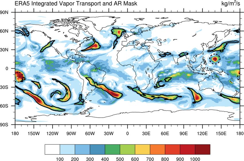
5024                                                                                P. A. Ullrich et al.: TempestExtremes v2.1

nodal (i.e., pointwise) and areal atmospheric features. Ap-            – It is designed to work with “big data”, enabling signif-
pendices A–C of Ullrich and Zarzycki (2017) summarized                   icant data volume reduction by isolating characteristics
dozens of such automated algorithms for extratropical cy-                of individual features rather than full fields.
clones, tropical cyclones, and tropical easterly waves. Even
so, work to identify optimal tracking criteria continues (Mu-          – Kernels are designed for arbitrarily grids, recognizing
rata et al., 2019). Beyond these traditionally tracked fea-              that climate models have largely moved away from
tures, many recent papers have focused on defining region-               latitude–longitude grids and towards quasi-uniform
ally relevant features such as monsoonal lows and depres-                grids (Ullrich et al., 2017).
sions associated with heavy precipitation in monsoonal re-             – All TE code is open-source, publicly developed, and
gions (Hurley and Boos, 2015; Vishnu et al., 2020). Areal                distributed via GitHub with permissive open-source li-
feature tracking algorithms have also been developed for                 censing.
clouds (Heikenfeld et al., 2019), atmospheric rivers (Shields
et al., 2018; Rutz et al., 2019), atmospheric blocking (Scher-     These principles complement the underlying foci motivating
rer et al., 2006), mesoscale convective systems (Prein et al.,     TE’s development: robustness, usability, maintainability, and
2017; Feng et al., 2018), precipitation clusters (Clark et al.,    extensibility. To the best of the authors’ knowledge, no other
2014; Pendergrass et al., 2016), convectively generated out-       comprehensive toolkit exists for general nodal and areal fea-
flow boundaries (Chipilski et al., 2018), gust fronts (Delanoy     ture tracking in Earth system datasets.
and Troxel, 1993), and frontal systems (Hope et al., 2014;            The remainder of this paper follows an analogous struc-
Schemm et al., 2015; Parfitt et al., 2017). Both nodal and         ture to Ullrich and Zarzycki (2017). Section 2 describes the
areal algorithms generally feature a similar set of kernels,       core algorithms and kernels now available in TE v2.1. Sec-
motivating the development of a single package encompass-          tion 3 presents several examples of how these kernels can
ing relevant capabilities. For example, the majority of de-        be combined to form recipes for tracking tropical cyclones
tection algorithms are built upon an algorithmic paradigm          (TCs), for calculating fractional contribution of precipitation
known as MapReduce (Dean and Ghemawat, 2008), in which             from TCs, for tracking and compositing extratropical cyclone
individual time slices are independently assessed (an em-          fields, for tracking atmospheric rivers, and for tracking at-
barrassingly parallel “map” operation) then combined via a         mospheric blocks. A summary of results and future work is
serial “reduce” operation. By building a single framework          given in Sect. 4.
for distributing time slices to different feature identification
algorithms, then combining multiple features into a single
                                                                   2     TempestExtremes algorithms and kernels
dataset, we can avoid duplication of this infrastructure across
multiple trackers. Leveraging commonalities such as these          In this section we describe the kernels available in the TE
enables improvements in algorithmic efficiency to be simul-        software package, organized by executable, with an emphasis
taneously administered to multiple trackers and reduces re-        on additions since TE v1.0. Technical details on the operation
dundancies from algorithmic validation and testing.                of TempestExtremes can be found in the user guide (Ullrich,
   TE has been engineered with the goal of providing a com-        2020).
prehensive and user-friendly toolbox for feature tracking in
model, reanalysis, or observational data products. It features     2.1    DetectNodes and StitchNodes
a set of core design principles to enable its easy application
in scientific analyses:                                            DetectNodes (formerly DetectCyclonesUnstructured) is used
                                                                   for the detection of nodal feature candidates and corresponds
  – Kernels are encapsulated in a variety of executables that      to the parallel “map” step in the “MapReduce” framework
    are fully configurable from the command line (i.e., con-       – that is, candidate points are selected based on informa-
    taining no hard-coded thresholds). Thus the process-           tion at a single time slice. DetectNodes is typically followed
    ing operations performed by TE can be easily conveyed          by StitchNodes, which represents the serial “reduce” oper-
    simply by communicating the relevant command(s).               ation in the processing chain. StitchNodes connects nodal
  – Many of the finer details about the structure of climate       features in time and produces paths associated with singular
    datasets are abstracted through the use of physically mo-      features. Both of these executables and their algorithmic ker-
    tivated kernels (such as the closed contour operator),         nels are described in Ullrich and Zarzycki (2017), although
    physically based units, and internal indexing with cli-        version 2.1 now supports the use of physical time units for
    mate and forecast (CF) compliant time variables.               thresholds and time subsetting. For example, mintime may
                                                                   be specified as a minimum number of time slices (e.g., “5”)
  – The data analysis capabilities are designed to be high-        or as the minimum number of hours between the first and last
    throughput, readily usable, and standardized. All TE           candidate in a path (e.g., “24h”).
    functionality is implemented in optimized and (where              DetectNodes and StitchNodes output trajectories in a for-
    appropriate) parallelized C++.                                 mat originally defined by the Geophysical Fluid Dynamics

Geosci. Model Dev., 14, 5023–5048, 2021                                             https://doi.org/10.5194/gmd-14-5023-2021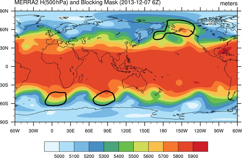
P. A. Ullrich et al.: TempestExtremes v2.1                                                                                               5025

Table 1. Functions implemented in NodeFileEditor as of TempestExtremes v2.1.

  Operator               Description
  eval_ace               Calculate the instantaneous accumulated cyclone energy (ACE; Bell et al., 2000), equal to 10−4 u2kt,max , where
                         ukt,max is the maximum wind speed within a prescribed radius of the nodal feature in knots. We use a value of
                         1.94384 kn (m s−1 )−1 to convert meters per second (m s−1 ) to knots (kn).
  eval_acepsl            Approximate ACE using sea level pressure (SLP) to predict surface wind speed (ACEPSL). Currently, ACEPSL
                         is calculated as ACE but using ukt,max = 1.94384 kn (m s−1 )−1 ×3.92× (1016.0 hPa − slpmin )0.644 (Holland,
                         2008), where slpmin is the minimum SLP within a prescribed radius.

                         Calculate the instantaneous integrated kinetic energy (Powell and Reinhold, 2007), defined as i 21 u2i Ai , where
                                                                                                                         P
  eval_ike
                         ui is the magnitude of the wind speed at that grid cell (in m s−1 ), Ai is the area of that grid cell (in m2 ), and
                         the sum is taken over all grid cells within a prescribed radius.
  eval_pdi               Calculate the power dissipation index (Emanuel, 2005), defined as u3max , where umax is the maximum wind
                         speed within a prescribed radius (in m s−1 ).
  radial_profile         Develop a radial profile of the specified variable at each time slice around the nodal feature point by binning by
                         radial distance and averaging grid point values. The output is expressed using Python array syntax.
  radial_wind_profile    This is like radial_profile but for the radial and azimuthal wind speed. The radial and azimuthal components are
                         computed by projecting the 2D velocity at each grid point onto the radial and azimuthal vector fields around
                         each nodal feature prior to binning.
  last where             Given an array as input, such as the output of radial_profile, identify the distance or index of the array that
                         satisfies a given threshold. For example, this operator is used for determining the radius at which azimuthal
                         wind speed is greater than 8 m s−1 .
  value                  Given an array, extract the value at the specified index using linear interpolation where needed.
  max_closed_contour     For a given field, determine the largest value that satisfies the closed contour criteria (see Ullrich and Zarzycki,
                         2017, Sect. 2.6) around each nodal feature (see Algorithm 1).
  region_name            Given the names and coordinates of polygons in longitude–latitude space, identify the name of the region for a
                         given pointwise feature. Each point is identified as being in a given region using a straight-line test along lines
                         of constant latitude. If the number of intersections with edges of the polygon is odd (even), then the point is
                         inside (outside).

Laboratory (GFDL) tropical cyclone tracker (TSTORMS;                     provided in Algorithm 1. Intuitively, this algorithm can be
Vitart et al., 1997; Zhao et al., 2009). These files are gen-            thought of as filling up a 3D extruded surface representative
erally referred to as nodefiles.                                         of the contours of the field until fluid spills farther out than
                                                                         the prescribed maximum distance. The last height difference
2.2   NodeFileEditor                                                     is then recorded as the maximum delta for the closed contour.

                                                                         2.3   NodeFileFilter
NodeFileEditor is a new addition to TE for editing nodefiles.
It includes options for (1) appending new details to trajecto-           NodeFileFilter encapsulates algorithms for masking spatial
ries, such as radial wind profiles or accumulated cyclone en-            data using nodefile information, i.e., effectively converting
ergy, (2) removing certain columns from nodefiles, or (3) fil-           nodefiles into binary raster masks at each time slice and (op-
tering trajectories or points along a trajectory, e.g., when out-        tionally) applying them to available data. Filtering can be
side of a specific time interval. A list of functions currently          performed using the distance from each feature, based on the
available in NodeFileEditor is given in Table 1. These func-             closed contour of each feature (as described by Algorithm 2),
tions may be chained to perform multiple related operations,             or by thresholding of areal regions that are within a given
such as computing a radial wind profile of a tropical cyclone            distance of each nodal feature (as described by Algorithm 3).
and then extracting the radius where a particular wind thresh-           The latter is useful for identifying, for instance, precipitation
old is exceeded. An example of such chaining of commands                 clusters associated with tropical cyclones.
is given in Sect. 3.3.
   Most of the implemented algorithms are straightforward,
except for max_closed_contour, whose pseudo-code is

https://doi.org/10.5194/gmd-14-5023-2021                                                     Geosci. Model Dev., 14, 5023–5048, 2021
5026                                                                               P. A. Ullrich et al.: TempestExtremes v2.1

2.4    NodeFileCompose                                            at a single time slice, typically simple thresholds such as “all
                                                                  points where precipitation is greater than 1 mm d−1 ”. Fea-
NodeFileCompose includes functionality for snapshotting           tures are marked using a binary mask and output stored in
fields around nodal features (i.e., at each time slice project-   NetCDF format. Contiguous regions may then be excluded
ing fields onto the stereographic plane centered on a nodal       based on either geometric thresholds or criteria derived from
feature) or compositing fields (i.e., averaging snapshots). In    other variables. DetectBlobs supports MPI-based (message
the same vein, it also includes functionality for snapshotting    passing interface) parallelism over input files.
or compositing a particular geographic region when a fea-
ture is present. Stereographic composites are computed using
                                                                  2.6   StitchBlobs
Algorithm 4. The mathematical operators used for the local
stereographic projection are given in Appendix A.
                                                                  StitchBlobs is used for tracking areal features (blobs) in time,
2.5    DetectBlobs                                                assigning connected features a unique global ID and/or ap-
                                                                  plying time-dependent criteria to each contiguous region.
DetectBlobs is used for identifying areal features (blobs),       Given input as a time-dependent binary mask variable, blobs
such as atmospheric blocks, atmospheric rivers, or precip-        that overlap at sequential time steps will be assigned the same
itation clusters. As with DetectNodes, this executable rep-       global identifier. The algorithm implemented in TE for con-
resents the parallel “map” step in the “MapReduce” frame-         necting blobs in time uses a forward–backward search that
work. Candidate regions are selected based on information         can treat the “2D space + 1D time” object as a single 3D ob-

Geosci. Model Dev., 14, 5023–5048, 2021                                           https://doi.org/10.5194/gmd-14-5023-2021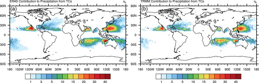
P. A. Ullrich et al.: TempestExtremes v2.1                                                                                    5027

                                                                       The pseudo-code for this search protocol is provided in al-
                                                                   gorithms 5 and 6, and its operation is illustrated in Fig. 1.
                                                                   Put briefly, contiguous regions at each time slice are iden-
                                                                   tified using a flood fill algorithm and assigned a unique tag
                                                                   of the form (time ID, blob ID). An additional “merge dis-
                                                                   tance” argument can be specified that merges nearby blobs
                                                                   at each time slice if their perimeters are within this speci-
                                                                   fied distance. A graph is then constructed with each of these
Figure 1. A depiction of algorithms 5 and 6 for forward–backward   tags corresponding to the nodes of the graph. Edges are then
areal feature search used by StitchBlobs, simplified to show one   added to the graph where a pair of areal features are deemed
space dimension (e.g., longitude) and the time dimension.          to be connected in time. Since multiple edges could be gener-
                                                                   ated to or from a feature on a given time slice, multiple merg-
                                                                   ers or splits may occur simultaneously. Finally, the compo-
                                                                   nents of the graph are each assigned a unique global ID, with
                                                                   lower global IDs corresponding to blobs that first appear at
ject, allowing for both splitting and merging of features in       earlier times. In Fig. 1, features at time index 1, denoted (1,1)
time.

https://doi.org/10.5194/gmd-14-5023-2021                                             Geosci. Model Dev., 14, 5023–5048, 2021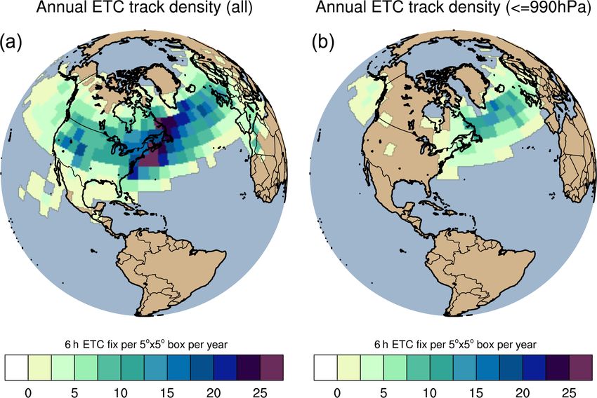
5028                                                                                P. A. Ullrich et al.: TempestExtremes v2.1

and (1,2), will both be assigned the same global ID since they     produce composite tracking and analysis algorithms. In all
are connected at a later time. Similarly, features at time index   examples, the corresponding TE commands are provided to
3, denoted (3,1) and (3,2), are assigned the same global ID        both demonstrate that they are effective at conveying the op-
since they were connected at an earlier time. Note that global     eration in a human-readable manner and to enable repro-
IDs start at 1 and are consecutive thereafter; they are assigned   ducibility of our results. Past examples from the literature
only after connected components of the graph are identified        using TE are provided in Sect. 3.1. This is then followed
and as such are unrelated to the blob ID on each time slice.       by several examples from TE of feature-based tracking and
   By default, areal features are deemed to be connected in        subsequent analysis. These examples include TC tracking in
time if they share at least one grid point at subsequent time      ERA5, fractional contribution of precipitation from TCs in
steps (regardless of the area of that grid point). For example,    ERA5 and Tropical Rainfall Measuring Mission (TRMM),
in Fig. 1, areal regions (1,1) and (2,1) overlap in space and      atmospheric river tracking in ERA5, extratropical cyclone
so are deemed to be connected. If a stricter threshold on the      tracking in CMIP6 data, and finally generation of an atmo-
overlap area is needed for blobs at sequential time slices to      spheric blocking climatology using MERRA2 data.
be deemed part of the same cluster, StitchBlobs provides ar-
guments for minimum overlap between the current blob and           3.1   Examples from the existing literature
blobs at the previous and/or next time step. In this exam-
ple, blob tag (2,2) overlaps only 25 % of the area of blob tag     Since version 1.0, TE has been employed for feature tracking
(1,2), meaning that (2,2) and (1,2) are deemed unconnected         in a number of scientific studies. Here we catalogue known
if the “minimum previous overlap” is greater than 25 %. On         publications emerging from those studies, organized by fea-
the other hand blob tag (1,2) covers 50 % of the area of blob      ture type.
tag (2,2), so these two would be deemed unconnected if the            Tropical Cyclones (TCs). More than any other feature, TE
“minimum next overlap” is greater than 50 %.                       has been employed for the study of TCs. TE was first em-
                                                                   ployed as a TC tracker to understand intensity errors associ-
2.7    Other utilities                                             ated with one-way coupling between ocean and atmosphere
                                                                   in Zarzycki (2016). It was subsequently used to investigate
In addition to the core functionality described in previous        the TC wind–pressure relationship in Chavas et al. (2017), a
sections, TE also provides a number of other utilities to man-     relationship later revisited in Moon et al. (2020) in which TE
age nodefiles, binary masks, and other climatological data         was used to assess its sensitivity to model resolution. In Wing
relevant to feature tracking. These are briefly mentioned here     et al. (2019), TE was applied to native grid data produced
as this functionality is employed in the composite tracking        using the Community Atmosphere Model Spectral Element
algorithms and analysis of Sect. 3.                                (CAM-SE) dynamical core to track TCs; outputs were then
    – Climatology is used for constructing climatological time     used to investigate the processes underlying moist intensifi-
      series, including long-term daily, monthly, seasonal, and    cation of TCs. A related study by Camargo et al. (2020) used
      annual means. It supports parallel execution over files      this dataset to investigate the large-scale environment around
      via MPI, as well as arguments that can be used to limit      TCs. In Roberts et al. (2020a) and Roberts et al. (2020b), TE-
      the amount of memory used by each thread.                    derived TC tracks were used to understand resolution sensi-
                                                                   tivity and future change in both historical and future High-
    – FourierFilter is used for Fourier filtering/smoothing of     ResMIP experiments (Haarsma et al., 2016) across several
      input data series. Although it provides a general imple-     models. Along these lines, Balaguru et al. (2020) used TE
      mentation that could be used for any dataset, it has pri-    to characterize TC climatology in the Energy Exascale Earth
      marily been used for smoothing long-term daily means         System Model (E3SM). Reed et al. (2020, 2021) used TE
      produced from Climatology.                                   to extract tracks of hurricanes Florence (2018) and Dorian
                                                                   (2019) and attribute human influence on these storms. TE
    – VariableProcessor provides direct access to TE’s inter-
                                                                   has also been used for tracking storms in aquaplanet simula-
      nal variable processing capability, allowing arithmetic
                                                                   tions (Chavas and Reed, 2019) so as to better understand how
      and grid-based operations to be applied to gridded data
                                                                   dynamic forcing impacts TC genesis and size. Recent work
      files. The operation of this utility is roughly analogous
                                                                   by Stansfield et al. (2020) has also leveraged some of the
      to that of the NetCDF Operator ncap2 (NCO; Zender,
                                                                   more advanced capabilities in TE to filter fields (e.g., precip-
      2008).
                                                                   itation) in the vicinity of tracked features to evaluate model
                                                                   performance. TE has also been used for the tracking of TCs
3     Selected examples                                            in extremely high-resolution regional simulations (Steptoe
                                                                   et al., 2021) and investigating TCs in paleoclimate simula-
In this section we present several examples of tracking and        tions (Kiehl et al., 2021).
analysis of different features; that is, different recipes for        Extratropical Cyclones (ETCs). In order to better under-
combining the algorithmic kernels described in Sect. 2 to          stand cyclonic storms and their impacts, Zarzycki et al.

Geosci. Model Dev., 14, 5023–5048, 2021                                            https://doi.org/10.5194/gmd-14-5023-2021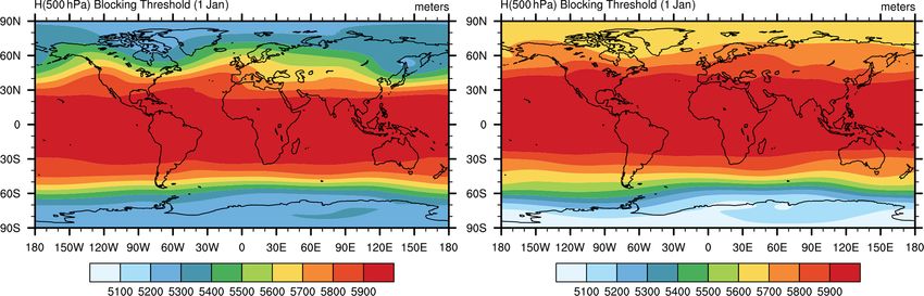
P. A. Ullrich et al.: TempestExtremes v2.1                                                                              5029

(2017) developed the ExTraTrack software framework atop         compared with trackers based on sea level pressure, vortic-
TE to track TCs and ETCs through their entire life cycle.       ity, and geopotential. A weighted critical success index (CSI)
This module enabled cyclonic storms to be examined us-          (Di Luca et al., 2015) was used to determine tracker perfor-
ing the thermal wind and thermal asymmetry phase space of       mance. However, acknowledging the possibility of errors in
Hart (2003). ExTraTrack was later applied to a suite of high-   the reference dataset (here the Sikka archive), the weighted
resolution global simulations in Michaelis and Lackmann         CSI index used in this analysis also considered the degree to
(2019) and Michaelis and Lackmann (2021). ETCs were also        which a track is represented similarly across all reanalyses.
tracked in the Community Earth System Model Large En-           A related study by Zhang et al. (2019) also tracked tropical
semble (CESM-LENS) in Zarzycki (2018) to understand the         depressions in the North Indian Ocean in 2018 to investigate
drivers responsible for snowstorms in the US northeast. Then    the anthropogenic impact on this storm season, and a recent
in Small et al. (2019), extratropical storms tracked using TE   study by You and Ting (2021) used TE to assess trends in
were used to determine if resolving ocean fronts improves       South Asian Monsoon low-pressure systems.
the representation of simulated storm tracks. In Zhang et al.      Atmospheric blocking. In Pinheiro et al. (2019), a suite
(2021) the vertical symmetry criterion from ExTraTrack was      of atmospheric blocking methods from TE were applied to
also adapted for the tracking of Mediterranean hurricanes       ERA-Interim data to better understand sensitivities of atmo-
(medicanes). Finally, TE was also used to track ETCs as part    spheric blocks to the detection algorithm and the meteoro-
of an effort to evaluate severe local storm environments in     logical environment around blocking features.
climate models and reanalysis (Li et al., 2020).                   Atmospheric rivers (ARs). Atmospheric river tracking with
   Monsoonal lows and depressions. Analogous to the study       TE was first documented as part of the Atmospheric River
of Zarzycki and Ullrich (2017), Vishnu et al. (2020) opti-      Transport Method Intercomparison Project (ARTMIP) in
mized DetectNodes for the tracking of monsoon lows and          Shields et al. (2018) and later in Rutz et al. (2019). The
depressions. A comprehensive analysis of input fields found     proposed algorithm used the Laplacian of the integrated va-
that 850 hPa streamfunction tended to produce better results    por transport (IVT) field rather than the IVT field itself,

https://doi.org/10.5194/gmd-14-5023-2021                                          Geosci. Model Dev., 14, 5023–5048, 2021
5030                                                                              P. A. Ullrich et al.: TempestExtremes v2.1

thus flagging IVT “ridges” rather than IVT over a thresh-         ucts. In this section we apply the same configuration that
old; this choice addressed issues of stationarity generally       provided maximal agreement between earlier-generation re-
present in trackers using an IVT threshold. TE’s algorithm        analyses and IBTrACS to ERA5 input (Hersbach et al., 2020)
has since been used both for AR detection and tracking (with      so as to identify ERA5 TC tracks.
DetectBlobs and StitchBlobs) in several subsequent studies
(Rhoades et al., 2020b, a; Patricola et al., 2020; McClenny       3.2.1   Step 1: identify candidate storms
et al., 2020; Huang et al., 2021; Zhou et al., 2021).
                                                                  Tropical cyclone tracking is an exemplar of the MapReduce
                                                                  paradigm discussed earlier in this paper. Essentially all pub-
3.2    Tropical cyclone tracking in ERA5                          lished algorithms for TC tracking (e.g., Ullrich and Zarzy-
                                                                  cki, 2017, their Appendix B) make use of a two-step process
In Zarzycki and Ullrich (2017), a sensitivity analysis was car-   consisting of first detecting TC candidates, then stitching to-
ried out to optimize TE for the detection of tropical cyclones    gether candidates in time. Both steps of this process include
by benchmarking hit rate (HR) and false alarm rate (FAR)          hard thresholds that separate TCs from related features. Al-
from reanalysis products against the International Best Track     though TE allows users to vary the values of these thresholds,
Archive for Climate Stewardship (IBTrACS; Knapp et al.,           here we only consider one such variation of these parameters.
2010). The resulting configuration, which tracked storms             In the TC detection algorithm described in Zarzycki and
based on sea level pressure minimum, produced the high-           Ullrich (2017), candidates are defined as points that have
est HR minus FAR differential in the literature across a          both a sea level pressure minimum and an upper-level warm
wide range of reanalysis products. An interesting result that     core. These conditions are codified via the following com-
emerged from this analysis was that upper-level geopotential      mand:
layer thickness (typically Z300 minus Z500) was the most
robust indicator of an upper-level warm core across prod-

Geosci. Model Dev., 14, 5023–5048, 2021                                           https://doi.org/10.5194/gmd-14-5023-2021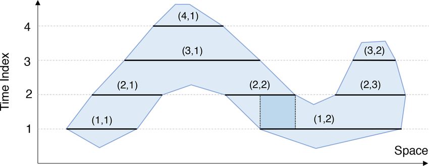
P. A. Ullrich et al.: TempestExtremes v2.1                                                                                 5031

DetectNodes                                                        protocol are eliminated if a stronger minimum exists within
--in_data_list ERA5_TC_files.txt                                   6◦ GCD.
--timefilter "6hr"                                                     The remaining argument outputcmd indicates three
--out_file_list ERA5_DN_files.txt                                  additional outputs that are calculated and written as ad-
--searchbymin MSL                                                  ditional columns in each nodefile. Here “MSL,min,0”
--closedcontourcmd "MSL,200.0,5.5,0;                               outputs the value of MSL at the candidate point,
             _DIFF(Z(300hPa),Z(500hPa)),                           “_VECMAG(VAR_10U,VAR_10V),max,2” outputs the
             -58.8,6.5,1.0"                                        maximum magnitude of the vector wind at 10 m altitude
--mergedist 6.0                                                    within 2◦ GCD of the candidate, and “ZS,min,0” outputs
--outputcmd "MSL,min,0;                                            the surface height at the candidate point. These variables are
      _VECMAG(VAR_10U,VAR_10V),                                    needed in the subsequent StitchNodes step to construct and
       max,2;ZS,min,0"                                             filter TC trajectories.

   For this example, our ERA5 data come from the National          3.2.2   Step 2: connect candidate storms in time
Center for Atmospheric Research (NCAR) Research Data
Archive (European Centre for Medium-Range Weather Fore-            Once TC candidates have been identified on each time slice,
casts, 2019), with 3D time-series data provided at hourly          the “stitching” step in the algorithm ties these candidates
resolution in daily chunks, 2D time-series data provided at        together in time to form TC trajectories (the “Reduce” op-
hourly resolution in monthly chunks, and 2D invariant data         eration in the MapReduce paradigm). Some features that
provided in a single file. The timefilter argument here            are too weak, too short-lived, or too disorganized are elim-
indicates that data should be downselected to 6-hourly, which      inated from contention at this stage. Also, features that are
is typical for analyses of TCs. As different variables are dis-    more likely related to topographic anomalies rather than real
tributed across multiple files, the first two lines of the input   storms are also removed.
data consist of several files containing 3D geopotential height       To build these trajectories with TE, we apply the
on pressure surfaces (Z), 2D mean sea level pressure (MSL),        StitchNodes command to the output from step 1:
2D 10 m zonal and meridional wind speeds (VAR_10U and
VAR_10V), and surface elevation (ZS), separated by semi-           StitchNodes
colons. Note that TE supports different agglomerations of          --in_list ERA5_DN_files.txt
time slices as it uses the CF-compliant time to match time         --out ERA5_TC_tracks.txt
slices across files.                                               --in_fmt "lon,lat,slp,wind,zs"
   To first limit the search space of possible TCs, we iden-       --range 8.0 --mintime "54h"
tify candidates as local minima in the sea level pressure          --maxgap "24h"
field. Two closed contour criteria are used to eliminate can-      --threshold "wind,>=,10.0,10;
didates. As argued in Ullrich and Zarzycki (2017), closed                         lat,=,-50.0,10;
defining features since they can be employed for both dis-                        zs,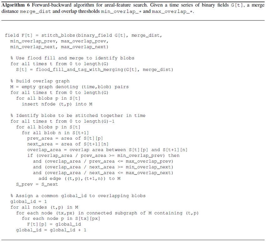
5032                                                                                     P. A. Ullrich et al.: TempestExtremes v2.1

Figure 2. Tropical cyclone trajectories from ERA5 (a) and IBTrACS (b) over the period 1980–2019, inclusive. TempestExtremes is used to
track TCs in ERA5, while pointwise observations are used for IBTrACS. Coloring denotes the instantaneous Saffir–Simpson category of the
tropical cyclone. The categories are computed from sea level pressure and applying the pressure–wind relationship of Atkinson and Holliday
(1977) with updated coefficients from Knaff and Zehr (2007). The discontinuity at 180◦ longitude in the bottom panel is due to historical
forecast center responsibilities.

   Four field-dependent thresholds are then specified                  datasets (Chavas et al., 2017). With that said, this proce-
for a trajectory to be accepted. The first threshold                   dure may overestimate storm intensity at higher latitudes
“wind,>=,10.0,10” indicates that the wind magni-                       where storms are beginning to undergo extratropical transi-
tude (derived from the “wind” column in the nodefile)                  tion. While tracked storms in ERA5 are generally too weak
must be greater than 10 m s−1 for at least 10 time slices;             in aggregate (lower density of orange and red trajectories in
this ensures that these features are sufficiently intense to           top panel), a common problem amongst reanalyses (Schenkel
be classified as tropical storms. The next two thresholds              and Hart, 2012; Murakami, 2014; Hodges et al., 2017), the
“lat,=,-50.0,10” indicate that                         method shows a high spatial and temporal correlation of
the latitude of the feature must be between 50◦ S and 50◦ N            storm climatology when compared to pointwise observa-
for at least 10 time slices, so as to eliminate any extratrop-         tions, and it produces superior hit rates (78 % for all TCs and
ical features that could not have existed as tropical storms.          95 % for those with wind speeds exceeding 33 m s−1 ) and
The final threshold “zs,
P. A. Ullrich et al.: TempestExtremes v2.1                                                                                   5033

3.3     Fractional contribution of precipitation from TCs               The calculations requested from NodeFileEdi-
                                                                     tor are specified by the calculate argument,
For the examples here, we calculate the fractional contri-           executed from left to right. First the radial pro-
bution of precipitation from TCs for one reanalysis dataset,         file is computed with radial_wind_profile
ERA5, and one observational dataset, the Tropical Rainfall           (VAR_10U,VAR_10V,159,0.125) and stored in
Measuring Mission (TRMM3B42; Huffman et al., 2007).                  variable rprof. These arguments indicate which variables
For ERA5, the TC track files are created as described in             should be used for the calculation and that the radial profile
Sect. 3.2. For TRMM, the IBTrACS dataset is used for TC              should consist of 159 bins of width 0.125◦ GCD. After the
track observations. Because there are limited comprehensive          radial profile is calculated, the last value where the radial
and long-term observational datasets of complete TC wind             wind profile is greater than 8 m s−1 is located and written
fields, ERA5 wind field data are combined with IBTrACS to            to the nodefile. The last value in the array is taken because
calculate the outer radius at every time step for all historical     we want to avoid recording the radius of the 8 m s−1 wind
TC tracks for the TRMM analysis.                                     within the TC inner core. The number of bins and the bin
                                                                     width were chosen based on the horizontal grid spacing of
3.3.1    Step 1: compute the outer radius of each tracked            the ERA5 wind data, which is approximately 31 km. The
         TC                                                          bin width of 0.125◦ adequately samples points at this grid
                                                                     spacing to create the radial wind profiles. The number of
As argued by Schenkel et al. (2017), the largest radius outside
                                                                     bins ensures the radial averaging extended out far enough
of the eyewall where the azimuthally averaged wind speed
                                                                     from the TC center points to capture the storms’ complete
exceeds 8 m s−1 (r8) tends to be a good measure of the size
                                                                     wind circulations.
of a TC. In Stansfield et al. (2020), TE was used to examine
the distribution of r8 among TCs in reanalysis data in ERA5          3.3.2   Step 2: build a mask using the outer radius of the
and a series of runs with the Community Earth System Model                   storm
(CESM). They further compared and contrasted TC-related
precipitation within r8 against precipitation within a fixed         With the r8 value for each TC now in hand, we define “TC-
distance of 500 km. We thus follow Stansfield et al. (2020)          related precipitation” as any precipitation which occurs at
and use r8 as our criterion for grid points to be part of the        grid points that are considered part of a TC. Employing TE’s
TC.                                                                  NodeFileFilter command, precipitation outside of the circle
   To begin, radial profiles and radius of 8 m s−1 wind are          with radius r8 centered on each TC is set to zero:
added to the nodefile generated in Sect. 3.2.2 and the IB-
TrACS nodefile (not shown):                                          NodeFileFilter
                                                                     --in_nodefile ERA5_TC_radprofs.txt
NodeFileEditor                                                       --in_fmt "lon,lat,rsize,rprof"
--in_data_list ERA5_TC_files.txt                                     --in_data_list ERA5_precip_files.txt
--in_nodefile ERA5_TC_tracks.txt                                     --out_data_list ERA5_filtered_
--in_fmt "lon,lat,slp,wind,zs"                                                        precip_files.txt
--out_nodefile ERA5_TC_radprofs.txt                                  --var "PRECT"
--out_fmt "lon,lat,rsize,rprof"                                      --bydist "rsize"
--time_filter "6hr"
--calculate "rprof=radial_wind_profile                                  The input nodefile is the output nodefile from Node-
         (VAR_10U,VAR_10V,159,0.125);                                FileEditor, now augmented with the radius of 8 m s−1 winds.
          rsize=lastwhere(rprof,>,8)"                                The input data contain 6-hourly ERA5 precipitation data
                                                                     from the NCAR Research Data Archive (European Cen-
   The input to this operation includes the files contain-           tre for Medium-Range Weather Forecasts, 2019) under vari-
ing the 2D ERA5 10 m zonal and meridional wind speeds                able name PRECT. Precipitation in ERA5 is calculated from
(VAR_10U and VAR_10V) and the nodefile generated in                  hourly forecasts initialized from the analysis at 06:00 and
Sect. 3.2.2. As part of this analysis we also augment an IB-         18:00 UTC. Precipitation is converted from hourly to 6-
TrACS nodefile in a similar manner, using the IBTrACS TC             hourly by adding up the accumulated precipitation 3 h be-
tracks but ERA5 winds to estimate TC size (command not               fore and 3 h after the desired time steps of 00:00, 06:00,
shown here). As in Sect. 3.2.1, a time filter is used to only        12:00, and 18:00 UTC. For example, to calculate 6-hourly
analyze 6-hourly time slices of data. Internal to the execution      precipitation at 06:00 UTC, the precipitation from 03:00 to
of this command is the construction of a date object for each        09:00 UTC is added up. For the TRMM analysis, the TRMM
entry of the nodefile which is then cross-referenced against         precipitation data are originally 3-hourly, so before analy-
every time slice in the list of data files to find the correspond-   sis the TRMM data are summed into 6-hourly data. This is
ing field – in this way indexing is abstracted from the user.        done using a centered averaging method; so, for example,
                                                                     to calculate 6-hourly precipitation at 06:00 UTC, half of the

https://doi.org/10.5194/gmd-14-5023-2021                                               Geosci. Model Dev., 14, 5023–5048, 2021
5034 P. A. Ullrich et al.: TempestExtremes v2.1
03:00 UTC precipitation, all of the 06:00 UTC precipitation, 3.4.1 Step 1: generate extratropical cyclone trajectories
and half of the 09:00 UTC precipitation are added up. Output
consists of a sequence of NetCDF files, one for each input The algorithm applied here identifies cyclonic storms as sea
file, containing filtered precipitation. level pressure minima. To avoid topographic lows and fea-
The final argument specifies how the filtering is per- tures that are not meteorological in character, additional cri-
formed, in this case by distance using rsize. This proce- teria are imposed on the minimum lifetime and propaga-
dure only keeps precipitation grid point values that are within tion distance. Note that while the algorithm is highly sim-
this distance of each detected TC. Internally to NodeFile- ilar to that published in Zarzycki (2018), other ETC detec-
Filter, the mask is computed by employing a k-d tree (see tion algorithms analogous to those published in the Inter-
discussion in Ullrich and Zarzycki, 2017). comparison of Mid-Latitude Storm Diagnostics (IMILAST;
Neu et al., 2013) can be configured using TE’s command line
3.3.3 Results from the generated tropical cyclone options. These alternative approaches include tracking on
precipitation climatology low-level geopotential height minima or vorticity maxima,
filtering based on spatial gradients, and removing candidate
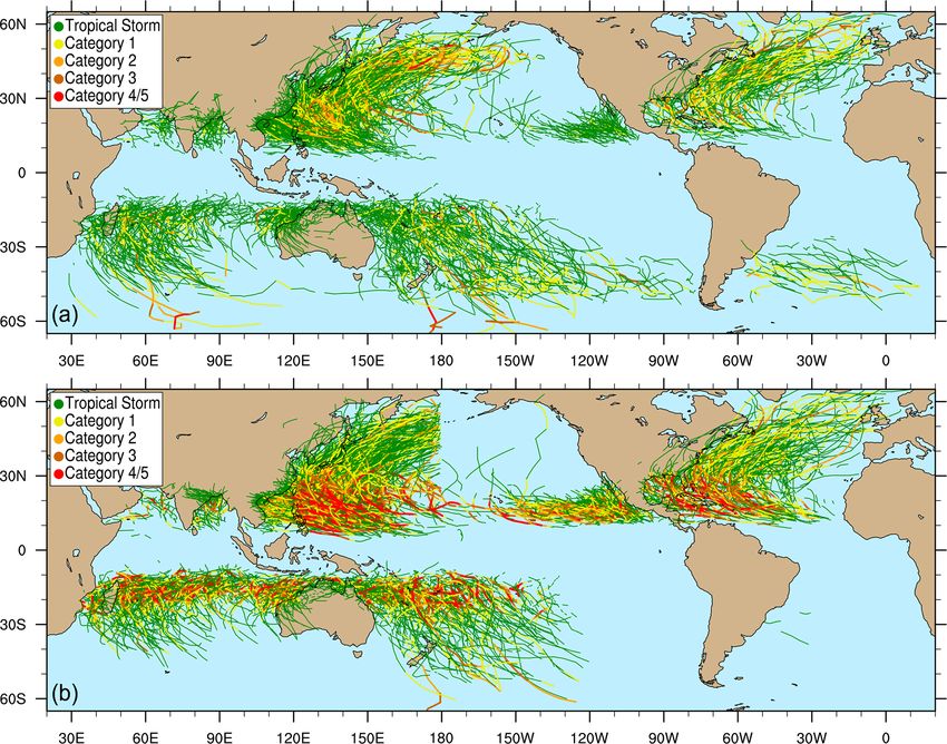
Figure 3 shows the relative contribution to global precipita- storms over higher terrain (see Table 1 in Neu et al., 2013).
tion from TCs for ERA5 and TRMM, calculated by using Also, while a more complex algorithm could help elimi-
NCO’s (NetCDF Operator) ncra to sum up the TC precip- nate cyclones that are tropical in nature (e.g., by using the
itation within r8 filtered by NodeFileFilter and dividing it no_closed_contour argument to eliminate candidates
by the sum of the total precipitation over the entire length with an upper-level warm core), none is applied here due to
of the datasets (1985–2019 for ERA5 and 1998–2014 for the relatively low resolution of CESM LENS. These coarser
TRMM). The areas of largest TC contribution align with the grid spacings are generally insufficient to resolve TCs (Walsh
areas of the highest TC activity shown in Fig. 2 and typi- et al., 2015), although higher-resolution evaluations of ETCs
cally occur over the ocean, in broad agreement with Prat and may require additional exclusionary thresholds to minimize
Nelson (2013). Khouakhi et al. (2017) (their Fig. 3b) made their inclusion in storm track datasets if desired.
a similar plot, except using land-based gauge data and for a To begin, cyclonic storms are identified using DetectN-
slightly different time period, and showed similar locations odes by following sea level pressure (here, PSL) minima in
of maximum contributions of 40 %–50 % over northwestern 6-hourly data:
Australia and eastern Asia.
DetectNodes
3.4 Extratropical cyclones --in_data_list B20TRC5CNBDRD.
001.PS_list.txt
Extratropical cyclones are midlatitude, synoptic-scale --out cyclone_candidates
weather features responsible for a host of impacts, including --closedcontourcmd "PSL,200.0,6.0,0"
high winds, coastal surge, and heavy precipitation, which --mergedist 6.0
can fall as rain, snow, sleet, or freezing rain (Schultz et al., --searchbymin "PSL"
2019; Dacre, 2020). Even though these features occur at --outputcmd "PSL,min,0"
relatively large spatial scales, models still have difficulty
in capturing hazards related to ETCs (e.g., Colle et al., Our criterion for cyclonic storms is that the minimum pres-
2015; Catalano et al., 2019), emphasizing the importance of sure must be enclosed by a closed contour of 200 Pa within
evaluating them at a process level in weather and climate 6.0◦ of cyclone center. This minimum pressure location also
datasets. defines the cyclone center. Candidates within 6.0◦ of one an-
Here we produce 2D composites of several fields asso- other are merged, with the lower pressure taking precedence.
ciated with ETCs tracked in the first historical member of Outputs from DetectNodes are then concatenated into a sin-
the Community Earth System Large Ensemble (Kay et al., gle candidate list, and StitchNodes is run to track these fea-
2015). ETCs over the northeastern United States were origi- tures in time:
nally analyzed in this dataset in Zarzycki (2018). The years
available for analysis in the historical simulations range from StitchNodes
1990 to 2015, inclusive. We also apply a pre-defined inten- --in_fmt "lon,lat,slp"
sity threshold and spatially constrain ETCs to pass over the --in_list candidate_list.txt
continental United States (CONUS) in order to demonstrate --out etc-all-traj.txt
a regional analysis and highlight both the filtering and com- --range 6.0
positing capabilities of TE. --mintime 60h
--maxgap 18h
--min_endpoint_dist 12.0
--threshold "lat,>,24,1;lon,>,234,1;
lat,P. A. Ullrich et al.: TempestExtremes v2.1 5035
Figure 3. Percent contribution to precipitation from tropical cyclones using precipitation field from (a) ERA5 and (b) TRMM.
moderate/weak ETCs as in Zhang and Colle (2017). To do
so, all ETCs tracked in step 1 are passed into NodeFileEd-
itor, in which a new trajectory file specified by argument
out_nodefile is generated with storms only possessing
intensities of 990 hPa or lower:
NodeFileEditor
--in_nodefile etc-all-traj.txt
--in_data_list B20TRC5CNBDRD.
001.PRECT_list.txt
--in_fmt "lon,lat,slp"
--out_fmt "lon,lat,slp"
--out_nodefile etc-strong-traj.txt
--colfilter "slp,5036 P. A. Ullrich et al.: TempestExtremes v2.1
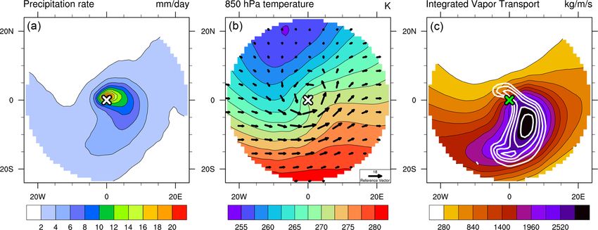
Figure 5. Composites of meteorological quantities centered on ETC storm center of all filtered storms with SLP less than or equal to 990 hPa
in the first CESM-LENS historical member. Shown from left to right are precipitation rate (mm d−1 ), 850 hPa temperature (K) with overlain
850 hPa wind vectors (m s−1 ), and integrated vapor transport (g kg−1 ) with overlain 600 hPa pressure velocity (omega) contours (every
hPa h−1 starting at −2 hPa h−1 ) . Each composite includes 11 164 data points.
--out_data_list B20TRC5CNBDRD. 3.4.4 Results from compositing extratropical cyclone
001.PRECT_FILT_list.txt fields
--var "PRECT"
--bydist 25.0 Figure 5 shows the composited precipitation rate field
--maskvar "mask" (PRECT), along with analogously calculated composites of
850 hPa temperature (T850) and integrated vapor transport
A binary variable named “mask” (as specified by argument (IVT). Total precipitation is largest near the storm center.
maskvar) is also included in the filtered files for reference Further, advection of warm, moist air wrapping cyclonically
and can be used for offline masking and visualization. around the eastern side of the storm center is seen in the
As a last step, storm-centered composites are generated 850 hPa temperature field (composite wind vectors shown in
using the following command: black). Lastly, the collocation of high values of IVT and ris-
NodeFileCompose ing motion in the mid-troposphere (600 hPa omega contours
--in_nodefile etc-strong-traj.txt shown in white) shows strong upward and poleward moisture
--in_fmt "lon,lat,slp" advection associated with the warm conveyor belt, as pre-
--in_data_list B20TRC5CNBDRD.001. viously shown in hand-compositing studies (e.g., Browning,
PRECT_FILT_list.txt 1986; Field and Wood, 2007).
--out_data "composite_PRECT.nc"
--var "PRECT" 3.5 Atmospheric rivers
--max_time_delta "2h"
--op "mean" Atmospheric rivers (ARs) are thin and long filamentary
--dx 1.0 structures characterized by high integrated vapor transport
--resx 80 (IVT; Payne et al., 2020). As found by Zhu and Newell
(1998), ARs are responsible for approximately 90 % of pole-
Here, only ETCs filtered above to have central SLP val- ward vapor transport. Our goal in this section is to reproduce
ues below 990 hPa are composited. Although we can com- this result in 20 years of ERA5 reanalysis using the Tempest
posite any 2D field, here we apply the compositing tool AR detection algorithm (Shields et al., 2018; Rhoades et al.,
to precipitation filtered by NodeFileFilter. The argument 2020b, a; McClenny et al., 2020).
max_time_delta indicates that the data slice nearest in
time to the tracked feature (within 2 h) should be compos- 3.5.1 Step 1: detect ridges in the IVT field
ited – this is useful when the discrete times from data and
features are not exactly aligned. The arithmetic mean is cal- As described in McClenny et al. (2020), the Tempest AR
culated centered on the storm location (see Sect. 2.4). The detection algorithm detects ARs as ridges in the IVT field,
resulting stereographic composite has a grid spacing of 1◦ where IVT is defined pointwise as
and a resolution of 80 × 80 grid points.
p
IVT = VIWVE2 + VIWVN2 . (1)
Geosci. Model Dev., 14, 5023–5048, 2021 https://doi.org/10.5194/gmd-14-5023-2021P. A. Ullrich et al.: TempestExtremes v2.1 5037
Here we have adopted the nomenclature of ERA5 for ver- --in_fmt "lon,lat,slp,wind,zs"
tically integrated eastward vapor transport (VIWVE) and --in_data_list ERA5_AR_files.txt
northward vapor transport (VIWVN). Ridge points are asso- --out_data_list ERA5_AR_NFF_files.txt
ciated with high downward curvature and identified as those --var "binary_tag"
points where the Laplacian of the IVT field is below a fixed --bydist 8.0
threshold (here chosen to be −2 × 10⁴ kg m−2 s−1 rad−2 ). --invert
These points are useful indicators of the presence of ARs
because this threshold identifies either long and narrow fea- Here the nodefile from ERA5 is specified by
tures or localized maxima (which are subsequently filtered in_nodefile and in_fmt. The input list of files contain-
using a minimum area criterion). Here the Laplacian is cal- ing the AR binary masks, specified with in_data_list, is
culated using eight radial points at a 10◦ GCD (as described the same as the output from DetectBlobs. The filtered output
in Appendix B); this large stencil on the Laplacian provides files are written to the file specified by out_data_list.
some smoothing of the field. Note that all field manipulation The last two arguments here are key to the filtering pro-
routines are handled by TE internally. The command for this cedure, specifying that the mask should include all points
operation is as follows: except those within 8◦ GCD of each nodal feature.
Figure 6 shows the ERA5 IVT field on 25 September 2019
DetectBlobs at 18:00 UTC, along with the outlines of AR objects detected
--in_data_list ERA5_IVT_files.txt using TE. On this date, an AR event was responsible for
--out_list ERA5_AR_files.txt flooding in California’s Russian River basin (seen here inter-
--timefilter "6hr" secting the US west coast). Dashed lines in this plot show the
--thresholdcmd "_LAPLACIAN{8,10} footprint of Super Typhoon Wutip at 15◦ N, 139.75◦ E and
(_VECMAG(VIWVE,VIWVN)),=,4e5km2" pear in IBTrACS until 26 February 2019 at 06:00:00 UTC.
The first three arguments refer to the list of input files and 3.5.3 Step 3: apply AR mask to northward vapor
output files and specify that data should be downsampled transport field
to 6-hourly time steps. The grid-point-level filtering opera-
tion is specified via the thresholdcmd argument, which To now investigate AR and non-AR poleward moisture
uses the gridded data processor kernel built into TE to in- transport, we apply the mask generated in step 2 to the
ternally process the eastward and northward components of VIWVN field (northward vapor transport). Here we lever-
the integrated vapor transport (VIWVE and VIWVN, respec- age the VariableProcessor executable, which allows us to
tively) during the tagging operation. Specifically, the oper- apply TE’s built-in operations on a set of input files.
ation specified here identifies candidate grid points using a Here the input file ERA5_VPIN.txt is the same as
threshold on the Laplacian of the IVT. This command first ERA5_AR_NFF_files.txt, except with the correspond-
calculates IVT using the vector magnitude operator and then ing ERA5 VIWVN file appended to each line. To perform
calculates the Laplacian of the resulting field. Only points the processing we apply the following command:
whose Laplacian is less than the threshold are retained. The
last two arguments are then used to remove features too near VariableProcessor
the Equator and those that are deemed too small: the latitude --in_data_list ERA5_VPIN.txt
of each tagged grid point must be at least 15◦ , and each blob --out_data_list ERA5_VPOUT.txt
must have a minimum area of 4×10⁵ km2 . Such filtering cri- --timefilter "6hr"
teria are typical for AR trackers (Shields et al., 2018). --var "_PROD(binary_tag,VIWVN);
_PROD(_DIFF(1,binary_tag),VIWVN)"
3.5.2 Step 2: filter out tropical cyclones --varout "VIWVN_PW_AR,VIWVN_PW_NONAR"
As noted in McClenny et al. (2020), tropical cyclones, which The var argument here is specified to leverage TE’s in-
also tend to exhibit large values of IVT, are sometimes picked ternal gridded variable processor. Since binary_tag only
up as part of the detection procedure. Although their contri- has value 0 or 1, the product of VIWVN and binary_tag
bution to poleward IVT is small, it is nonetheless desirable will capture points within ARs, whereas the product of
to exclude TCs from this calculation. This can be done using VIWVN and _DIFF(1,binary_tag) will capture points
the ERA5 TC tracks produced in Sect. 3.2 to filter out points not within ARs. These two variables are then written as
within a prescribed distance of each detected TC: VIWVN_AR and VIWVN_NONAR in the output file.
Once AR and non-AR northward IVT have been calcu-
NodeFileFilter lated on a grid point level, the final processing step is han-
--in_nodefile ERA5_TC_tracks.txt dled outside of TE. To do so we take the time average and
https://doi.org/10.5194/gmd-14-5023-2021 Geosci. Model Dev., 14, 5023–5048, 20215038 P. A. Ullrich et al.: TempestExtremes v2.1
Figure 6. ERA5 integrated vapor transport (IVT) field with AR mask (black outlines) from 25 September 2019 18:00 UTC. Tropical cyclones
that have been filtered from the AR mask are indicated with dashed black lines (8◦ radius GCD).
zonal average of the fields produced by VariableProcessor proximately 13 % of the total run time is spent applying the
using NCO’s robust record averaging (ncra) and weighted Laplacian operator, while 6 % (2 min and 10 s) is spent con-
averaging (ncwa) operators. structing the Laplacian. Again using 64 threads, NodeFile-
Filter required 50 s, while VariableProcessor required 14 min
3.5.4 Results from calculation of northward vapor and 14 s.
transport from AR and non-AR points
3.6 Atmospheric blocking
Figure 7 shows zonal mean northward IVT for AR and non- Our final example addresses the development of a climatol-
AR points (top row), along with the relative contribution ogy of atmospheric blocking frequency. Atmospheric block-
to northward IVT from ARs (bottom row). Note that be- ing events are synoptic-scale weather phenomena character-
cause it is a fractional quantity, the bottom row equivalently ized by persistent obstruction of the normal westerly flow
shows fractional contribution to poleward IVT. The top row and are associated with heat waves, cold spells, flooding, and
here is complementary to Fig. 14 (middle) in Rutz et al. drought (Glickman, 2012). In Pinheiro et al. (2019) (here-
(2019), which was computed with 6-hourly MERRA2 data. after PUG19), several 2D algorithms were compared for the
The agreement between these two results is reassuring and detection and characterization of blocking features. It was
confirms that the AR tracker employed in this section is con- found that the identification algorithm of Dole and Gordon
sistent with other trackers. In the lower figure we see that (1983) (hereafter DG83), which identifies blocks as anoma-
the AR contribution to poleward transport around 45◦ N and lously high values of geopotential height at 500 hPa (Z500),
45◦ S is indeed close to the 90 % value reported by Zhu and was a robust method for global block detection and charac-
Newell (1998), although this contribution then decays pre- terization. In this section we will employ TE to generate a
cipitously at more poleward latitudes. Note, however, that climatology of blocking events using the modified DG83 al-
this is in part because AR moisture transport is almost al- gorithm of PUG19 as applied to MERRA2 reanalysis data
ways poleward, whereas non-AR transport is a mix of both (Gelaro et al., 2017).
poleward and equatorward contributions.
The AR detector described in this section was run on 3.6.1 Step 1: generate the blocking threshold
the NERSC Cori supercomputer on two nodes with 32
threads per node (64 threads total). When run over the ERA5 Following PUG19, a grid point is defined as a candidate for
monthly data from January 1979 through February 2020 at being blocked if the Z500 field exceeds a threshold Z500
6-hourly temporal resolution with 494 monthly files, Detect- value. This threshold value must be specified as a function
Blobs required 34 min and 42 s. Again this run was largely of latitude, longitude, and time, given the geographical and
I/O bound, with 66 % of the total run time from file input. Ap- seasonal variations in Z500 climatology. PUG19 suggest a
Geosci. Model Dev., 14, 5023–5048, 2021 https://doi.org/10.5194/gmd-14-5023-2021P. A. Ullrich et al.: TempestExtremes v2.1 5039
Figure 7. (a, b) Northward IVT (IVTn) from AR and non-AR grid points. (c, d) Fractional contribution to IVTn from AR points by latitude.
threshold value equal to the daily mean Z500 plus the maxi- Here the missingdata argument is needed since the
mum of 100 m or 1.5 times the daily standard deviation of the 500 hPa pressure surface sometimes falls below the ground in
Z500 field. Given that only 40 years of MERRA2 reanalysis the vicinity of the Himalayas, which is indicated in MERRA2
are available, daily averaged data tends to be quite noisy, and with missing values. Note that, relevant to subsequent com-
so Fourier smoothing is employed in time and space. mands, Climatology automatically prepends the descriptor
MERRA2 stores the 3D geopotential height variable in “dailymean_” to the variable, so the final climatology is writ-
the inst3_3d_asm_Np dataset using variable name “H”. ten to variable “dailymean_H”.
For simplicity we assume that the input files contain a We now calculate the standard deviation of the
list of all files from this dataset from 1 January 1980 to H(500hPa) field using the VariableProcessor:
30 June 2020 (40.5 years). Within this dataset the 500 hPa
VariableProcessor
geopotential height variable can be specified by variable
--in_data "MERRA2_H_LTDM.nc;
name H(500hPa), in which the vertical index is determined
MERRA2_H2_LTDM.nc"
automatically by TE. The first step described in Pinheiro
--out_data "MERRA2_H_mean_stddev.nc"
et al. (2019) is the construction of a Fourier-filtered long-
--var "dailymean_H,
term daily mean (LTDM) climatology of the Z500 field and
_SQRT(_DIFF(dailymeansq_H,
its square. The Climatology executable is used in this step
_POW(dailymean_H,2)))"
and can be executed in parallel:
--varout "dailymean_H,stddev_H"
Climatology
We then apply a 4-mode Fourier filter to both the
--in_data_list MERRA2_H_files.txt
dailymean_H and stddev_H fields across the time di-
--out_data MERRA2_H_LTDM.nc
mension and a 2-mode Fourier filter to the stddev_H field
--var "H(500hPa)"
in the zonal direction:
--period "daily"
--type "mean" FourierFilter
--missingdata --in_data MERRA2_H_mean_stddev.nc
Climatology --out_data MERRA2_H_mean_stddev
--in_data_list MERRA2_H_files.txt _timesmoothed.nc
--out_data MERRA2_H2_LTDM.nc --var "dailymean_H,stddev_H"
--var "H(500hPa)" --dim "time"
--period "daily" --modes 4
--type "meansq" FourierFilter
--missingdata --in_data MERRA2_H_mean_stddev
https://doi.org/10.5194/gmd-14-5023-2021 Geosci. Model Dev., 14, 5023–5048, 2021You can also read