Gaia Data Release 2: first stellar parameters from Apsis - Max-Planck ...
←
→
Page content transcription
If your browser does not render page correctly, please read the page content below
Astronomy & Astrophysics manuscript no. GDR2_Apsis                                                                                      c ESO 2018
3 April 2018

              Gaia Data Release 2: first stellar parameters from Apsis
 René Andrae1 , Morgan Fouesneau1 , Orlagh Creevey2 , Christophe Ordenovic2 , Nicolas Mary3 , Alexandru Burlacu4 ,
 Laurence Chaoul5 , Anne Jean-Antoine-Piccolo5 , Georges Kordopatis2 , Andreas Korn6 , Yveline Lebreton7, 8 , Chantal
           Panem5 , Bernard Pichon2 , Frederic Thévenin2 , Gavin Walmsley5 , Coryn A.L. Bailer-Jones1?

       1
           Max Planck Institute for Astronomy, Königstuhl 17, 69117 Heidelberg, Germany
       2
           Université Côte d’Azur, Observatoire de la Côte d’Azur, CNRS, Laboratoire Lagrange, Bd de l’Observatoire, CS 34229, 06304
           Nice cedex 4, France
       3
           Thales Services, 290 Allée du Lac, 31670 Labège, France
       4
           Telespazio France, 26 Avenue Jean-François Champollion, 31100 Toulouse, France
       5
           Centre National d’Etudes Spatiales, 18 av Edouard Belin, 31401 Toulouse, France
       6
           Division of Astronomy and Space Physics, Department of Physics and Astronomy, Uppsala University, Box 516, 75120 Uppsala,
           Sweden
       7
           LESIA, Observatoire de Paris, PSL Research University, CNRS UMR 8109, Université Pierre et Marie Curie, Université Paris
           Diderot, 5 place Jules Janssen, 92190 Meudon
       8
           Institut de Physique de Rennes, Université de Rennes 1, CNRS UMR 6251, F-35042 Rennes, France

       Submitted to A&A 21 December 2017. Resubmitted 3 March 2018 and 3 April 2018. Accepted 3 April 2018

                                                                     ABSTRACT

       The second Gaia data release (Gaia DR2) contains, beyond the astrometry, three-band photometry for 1.38 billion sources. One band
       is the G band, the other two were obtained by integrating the Gaia prism spectra (BP and RP). We have used these three broad
       photometric bands to infer stellar effective temperatures, T eff , for all sources brighter than G = 17 mag with T eff in the range 3 000–
       10 000 K (some 161 million sources). Using in addition the parallaxes, we infer the line-of-sight extinction, AG , and the reddening,
       E(BP−RP), for 88 million sources. Together with a bolometric correction we derive luminosity and radius for 77 million sources. These
       quantities as well as their estimated uncertainties are part of Gaia DR2. Here we describe the procedures by which these quantities
       were obtained, including the underlying assumptions, comparison with literature estimates, and the limitations of our results. Typical
       accuracies are of order 324 K (T eff ), 0.46 mag (AG ), 0.23 mag (E(BP−RP)), 15% (luminosity), and 10% (radius). Being based on only
       a small number of observable quantities and limited training data, our results are necessarily subject to some extreme assumptions that
       can lead to strong systematics in some cases (not included in the aforementioned accuracy estimates). One aspect is the non-negativity
       contraint of our estimates, in particular extinction, which we discuss. Yet in several regions of parameter space our results show very
       good performance, for example for red clump stars and solar analogues. Large uncertainties render the extinctions less useful at the
       individual star level, but they show good performance for ensemble estimates. We identify regimes in which our parameters should
       and should not be used and we define a “clean” sample. Despite the limitations, this is the largest catalogue of uniformly-inferred
       stellar parameters to date. More precise and detailed astrophysical parameters based on the full BP/RP spectrophotometry are planned
       as part of the third Gaia data release.
       Key words. methods: data analysis – methods: statistical – stars: fundamental parameters – surveys: Gaia

1. Introduction                                                              tions and G-band photometry based on 22 months of mission
                                                                             observations. Of these, 1.33 billion sources also have parallaxes
The main objective of ESA’s Gaia satellite is to understand the              and proper motions (Lindegren et al. 2018). Unlike in the first
structure, formation, and evolution of our Galaxy from a detailed            release, Gaia DR2 also includes the integrated fluxes from the
study of its constituent stars. Gaia’s main technological advance            BP and RP spectrophotometers. These prism-based instruments
is the accurate determination of parallaxes and proper motions               produce low resolution optical spectrophotometry in the blue
for over one billion stars. Yet the resulting three-dimensional              and red parts of the spectra which will be used to estimate as-
maps and velocity distributions which can be derived from these              trophysical parameters for stars, quasars, and unresolved galax-
are of limited value if the physical properties of the stars remain          ies using the Apsis data processing pipeline (see Bailer-Jones
unknown. For this reason Gaia is equipped with both a low-                   et al. 2013). They are also used in the chromatic calibration of
resolution prism spectrophotometer (BP/RP) operating over the                the astrometry. The processing and calibration of the full spectra
entire optical range, and a high-resolution spectrograph (RVS)               is ongoing, and for this reason only their integrated fluxes, ex-
observing from 845–872 nm (the payload is described in Gaia                  pressed as the two magnitudes GBP and GRP , are released as part
Collaboration et al. 2016).                                                  of Gaia DR2 (see Fig. 1). The production and calibration of these
    The second Gaia data release (Gaia DR2, Gaia Collaboration               data are described in Riello et al. (2018). 1.38 billion sources in
et al. 2018b) contains a total of 1.69 billion sources with posi-            Gaia DR2 have integrated photometry in all three bands, G, GBP ,
 ?
     corresponding author, calj@mpia.de

                                                                                                                 Article number, page 1 of 29page.29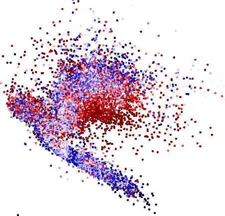
A&A proofs: manuscript no. GDR2_Apsis

and GRP (Evans et al. 2018), and 1.23 billion sources have both
five-parameter astrometry and three-band photometry.                                                  BP     G       RP

                                                                         transmission
    In this paper we describe how we use the Gaia three-band
photometry and parallaxes, together with various training data
sets, to estimate the effective temperature T eff , line-of-sight ex-
tinction AG and reddening E(BP−RP), luminosity L, and radius
R, of up to 162 million stars brighter than G=17 mag (some of
these results are subsequently filtered out of the catalogue). We
only process sources for which all three photometric bands are
available. This therefore excludes the so-called bronze sources                                            G2V                     M5III

                                                                         photon flux
(Riello et al. 2018). Although photometry for fainter sources is
available in Gaia DR2, we chose to limit our analysis to brighter                       Vega
sources on the grounds that, at this stage in the mission and
processing, only these give sufficient photometric and parallax
precision to obtain reliable astrophysical parameters. The choice
of G=17 mag was somewhat arbitrary, however.1 The work de-
                                                                                    2    3      4     5     6    7    8 9   103               2
scribed here was carried out under the auspices of the Gaia Data
Processing and Analysis Consortium (DPAC) within Coordina-                                          wavelength [nm]
tion Unit 8 (CU8) (see Gaia Collaboration et al. 2016 for an
                                                                          Fig. 1. The nominal transmissions of the three Gaia passbands (Jordi
overview of the DPAC). We realise that more precise, and pos-
                                                                          et al. 2010; de Bruijne 2012) compared with spectra of typical stars:
sibly more accurate, estimates of the stellar parameters could be         Vega (A0V), a G2V star (Sun-like star), and an M5III star. Spectral
made by cross-matching Gaia with other survey data, such as               templates from Pickles (1998). All curves are normalized to have the
GALEX (Morrissey et al. 2007), PanSTARRS (Chambers et al.                 same maximum.
2016), and WISE (Cutri et al. 2014). However, the remit of the
Gaia-DPAC is to process the Gaia data. Further exploitation, by
including data from other catalogues, for example, is left to the
community at large. We nonetheless hope that the provision of             arise from a mistake in our estimate, in the literature value, or in
these “Gaia-only” stellar parameters will assist the exploitation         both.
of Gaia DR2 and the validation of such extended analyses.
    We continue this article in section 2 with an overview of
our approach and its underlying assumptions. This is followed             2. Approach and assumptions
by a description of the algorithm – called Priam – used to in-            2.1. Overview of procedure
fer T eff , AG , and E(BP − RP) in section 3, and a description of
the derivation of L and R – with the algorithm FLAME – in                 We estimate stellar parameters source-by-source, using only the
section 4. The results and the content of the catalogue are pre-          three Gaia photometric bands (for T eff ) and additionally the par-
sented in section 5. More details on the catalogue itself (data           allax (for the other four parameters). We do not use any non-Gaia
fields etc.) can be found in the online documentation accompa-            data on the individual sources, and we do not make use of any
nying the data release. In section 6 we validate our results, in          global Galactic information, such as an extinction map or kine-
particular via comparison with other determinations in the liter-         matics.
ature. In section 7 we discuss the use of the data, focusing on                The three broad photometric bands – one of which is near
some selections which can be used to identify certain types of            degenerate with the sum of the other two (see Fig. 1) – provide
stars, as well as the limitations of our results. This is mandatory       relatively little information for deriving the intrinsic properties
reading for anyone using the catalogue. Priam and FLAME are               of the observed Gaia targets. They are not sufficient to deter-
part of a larger astrophysical parameter inference system in the          mine whether the target is really a star as opposed to a quasar or
Gaia data processing (Apsis). Most of the algorithms in Apsis             an unresolved galaxy, for example. According to our earlier sim-
have not been activated for Gaia DR2. (Priam itself is part of            ulations, this will ultimately be possible using the full BP/RP
the GSP-Phot software package, which uses several algorithms              spectra (using the Discrete Source Classifier in Apsis). As we
to estimate stellar parameters.) We look ahead in section 8 to            are only working with sources down to G=17, it is reasonable to
the improvements and extensions of our results which can be ex-           suppose that most of them are Galactic. Some will, inevitably,
pected in Gaia DR3. We summarize our work in section 9. We                be physical binaries in which the secondary is bright enough to
draw attention to appendix B, where we define a “clean” sub-              affect the observed signal. We nonetheless proceed as though all
sample of our T eff results.                                              targets were single stars. Some binarity can be identified in the
    In this article we will present both the estimates of a quantity      future using the composite spectrum (e.g. with the Multiple Star
and the estimates of its uncertainty, and we will also compare the        Classifier in Apsis) or the astrometry, both of which are planned
estimated quantity with values in the literature. The term uncer-         for Gaia DR3.
tainty refers to our computed estimate of how precise our esti-                Unsurprisingly, T eff is heavily degenerate with AG in the Gaia
mated quantity is. This is colloquially (and misleadingly) called         colours (see Fig. 2), so it seems near impossible that both quan-
an “error bar”. We provide asymmetric uncertainties in the form           tities could be estimated from only colours. Our experiments
of two percentiles from a distribution (upper and lower). We use          confirm this. We work around this by estimating T eff from the
the term error to refer to the difference between an estimated            colours on the assumption that the star has (ideally) zero extinc-
quantity and its literature estimate, whereby this difference could       tion. For this we use an empirically-trained machine learning
                                                                          algorithm (nowadays sometimes referred to as “data driven”).
 1
   The original selection was G ≤ 17 mag, but due to a later change in    That is, the training data are observed Gaia photometry of targets
the zeropoint, our final selection is actually G ≤ 17.068766 mag.         which have had their T eff estimated from other sources (generally
Article number, page 2 of 29page.29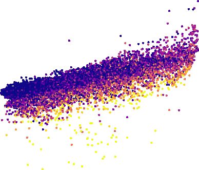
Andrae, Fouesneau, Creevey et al.: Gaia DR2: first stellar parameters from Apsis
1.50 (a) 9000 1.50 (b) 2.5
This is converted to a stellar luminosity using a bolometric cor-
rection (see section 4). The distance r to the target is taken sim-
G GRP [mag]
G GRP [mag]
1.25 8000 1.25
2.0
AG [mag]
1.00 1.00 ply to be the inverse of the parallax. Although this generally
Teff [K]
7000
0.75 0.75 1.5 gives a biased estimate of the distance (Bailer-Jones 2015; Luri
6000
0.50 0.50 1.0 et al. 2018), the impact of this is mitigated by the fact that we
5000
0.25 4000 0.25 0.5 only report luminosities when the fractional parallax uncertainty
0.00
3000
0.00
0.0
σ$ /$ is less than 0.2. Thus, of the 161 million stars with T eff
0 1 2 3 4 0 1 2 3 4 estimates, only 77 million have luminosity estimates included in
GBP G [mag] GBP G [mag] Gaia DR2.
Fig. 2. Colour–colour diagrams for stars from the PARSEC 1.2S models Having inferred the luminosity and temperature, the stellar
with an extinction law from Cardelli et al. (1989) and [Fe/H] = 0. Both radius is then obtained by applying the Stefan–Boltzmann law
panels use the same data, spanning A0 = 0–4 mag. We see that while T eff
is the dominant factor (panel a), it is strongly degenerate with extinction L = 4πR2 σT eff
4
. (3)
(panel b).
Because our individual extinction estimates are rather poor
for most stars (discussed later), we chose not to use them in the
Table 1. The photometric zeropoints used to convert fluxes to magni- derivation of luminosities, i.e. we set AG to zero in equation 2.
tudes via Eq. 1 (Evans et al. 2018). Consequently, while our temperature, luminosity, and radius es-
timates are self-consistent (within the limits of the adopted as-
band zeropoint (zp) [mag] sumptions), they are formally inconsistent with our extinction
G 25.6884 ± 0.0018 and reddening estimates.
GBP 25.3514 ± 0.0014 The final step is to filter out the most unreliable results: these
GRP 24.7619 ± 0.0020 do not appear in the catalogue (see appendix A). We furthermore
recommend that for T eff , only the “clean” subsample of our re-
sults be used. This is defined and identified using the flags in
appendix B. When using extinctions, users may further want to
spectroscopy). This training data set only includes stars which make a cut to only retain stars with lower fractional parallax un-
are believed to have low extinctions. certainties.
We separately estimate the interstellar absorption using the
three bands together with the parallax, again using a machine
2.2. Data processing
learning algorithm. By using the magnitudes and the parallax,
rather than the colours, the available signal is primarily the dim- The software for Apsis is produced by teams in Heidelberg, Ger-
ming of the sources due to absorption (as opposed to just the many (Priam) and Nice, France (FLAME). The actual execution
reddening). For this we train on synthetic stellar spectra, because of the Apsis software on the Gaia data is done by the DPCC
there are too few stars with reliably estimated extinctions which (Data Processing Centre CNES) in Toulouse, which also inte-
could be used as an empirical training set. Note that the absorp- grates the software. The processing comprises several opera-
tion we estimate is the extinction in the G-band, AG , which is tions, including the input and output of data and generation of
not the same as the (monochromatic) extinction parameter, A0 . logs and execution reports. The entire process is managed by
The latter depends only on the amount of absorption in the inter- a top-level software system called SAGA. Apsis is run in par-
stellar medium, whereas the former depends also on the spectral allel on a multi-core Hadoop cluster system, with data stored
energy distribution (SED) of the star (see section 2.2 of Bailer- in a distributed file system. The validation results are published
Jones 2011).2 Thus even with fixed R0 there is not a one-to-one on a web server (GaiaWeb) for download by the scientific soft-
relationship between A0 and AG . For this reason we use a sepa- ware providers. The final Apsis processing for Gaia DR2 took
rate model to estimate the reddening E(BP−RP), even though the place in October 2017. The complete set of sources (1.69 billion
available signal is still primarily the dimming due to absorption. with photometry) covering all Gaia magnitudes was ingested
By providing estimates of both absorption and reddening ex- into the system. From this the 164 million sources brighter than
plicitly, it is possible to produce a de-reddened and de-extincted G=17 mag were identified and processed. This was done on 1000
colour–magnitude diagram. cores (with 6 GB RAM per core), and ran in about 5000 hours
The inputs for our processing are fluxes, f , provided by the of CPU time (around five hours wall clock time). The full Ap-
upstream processing (Riello et al. 2018). We convert these to sis system, which involves much more CPU-intensive processes,
magnitudes, m, using higher-dimensional input data (spectra), and of order one billion
sources, will require significantly more resources and time.
m = −2.5 log10 f + zp (1)
where zp is the zeropoint listed in Table 1. All of our results
3. Priam
except T eff depend on these zeropoints.
We estimate the absolute G-band magnitude via the usual 3.1. General comments
equation
Once the dispersed BP/RP spectrophotometry are available, the
MG = G − 5 log10 r + 5 − AG . (2) GSP-Phot software will estimate a number of different stellar pa-
rameters for a range of stellar types (see Liu et al. 2012; Bailer-
2
We distinguish between the V-band extinction AV (which depends Jones et al. 2013). For Gaia DR2 we use only the Priam module
on the intrinsic source SED) and the monochromatic extinction A0 at a within GSP-Phot to infer parameters using integrated photom-
wavelength of λ = 547.7nm (which is a parameter of the extinction law etry and parallax. All sources are processed even if they have
and does not depend on the intrinsic source SED). corrupt photometry (see Fig. 4) or if the parallax is missing or
Article number, page 3 of 29page.29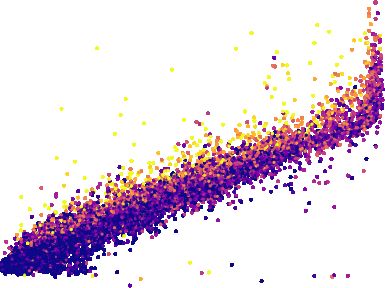
A&A proofs: manuscript no. GDR2_Apsis
non-positive. Some results are flagged and others filtered from Table 2. Catalogues used for training ExtraTrees for T eff estimation
the catalogue (see appendix A). showing the number of stars in the range from 3 000K to 10 000K that
we selected and the mean T eff uncertainty quoted by the catalogues.
Priam employs extremely randomised trees (Geurts et al.
2006, hereafter ExtraTrees), a machine learning algorithm with number mean T eff
a univariate output. We use an ensemble of 201 trees and take the catalogue of stars uncertainty [K]
median of their outputs as our parameter estimate.3 We use the APOGEE 5 978 92
16th and 84th percentiles of the ExtraTrees ensemble as two un- Kepler Input Catalogue 14 104 141
certainty estimates; together they form a central 68% confidence LAMOST 5 540 55
interval. Note that this is, in general, asymmetric with respect to RAVE 2 427 61
the parameter estimate. 201 trees is not very many from which RVS Auxiliary Catalogue 4 553 122
to accurately compute such intervals – a limit imposed by avail-
combined 32 602 102
able computer memory – but our validation shows them to be
reasonable. ExtraTrees are incapable of extrapolation: they can-
not produce estimates or confidence intervals outside the range
of the target variable (e.g. T eff ) in the training data. We exper- alogues we are deliberately “averaging” over the systematic dif-
imented with other machine learning algorithms, such as sup- ferences in their T eff estimates. The validation results presented
port vector machine (SVM) regression (e.g. Deng et al. 2012) in sections 5 and 6 will show that this is not the limiting factor
and Gaussian processes (e.g. Bishop 2006), but we found Ex- in our performance, however. This data set only includes stars
traTrees to be much faster (when training is also considered), which have low extinctions (although not as low as we would
avoid the high sensitivity of SVM tuning, and yet still provide have liked). 95% of the literature estimates for these stars are be-
results which are as good as any other method tried. low 0.705 mag for AV and 0.307 mag for E(B − V). (50% are be-
low 0.335 mag and 0.13 mag respectively.) These limits exclude
3.2. Effective temperatures the APOGEE part of the training set, for which no estimates of
AV or E(B − V) are provided. While APOGEE giants in partic-
Given the observed photometry G, GBP , and GRP , we use the ular can reach very high extinctions, they are too few to enable
distance-independent colours GBP −G and G−GRP as the inputs ExtraTrees to learn to disentangle the effects of temperature and
to ExtraTrees to estimate the stellar effective temperature T eff . extinction in the training process. The training set is mostly near-
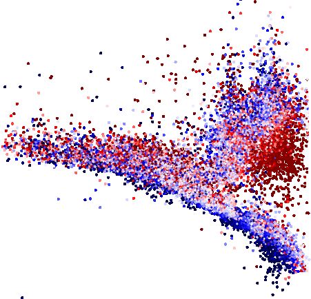
These two colours exhibit a monotonic trend with T eff (Fig. 3). solar metallicity stars: 95% of the stars have [Fe/H] > −0.82 and
It is possible to form a third colour, GBP − GRP , but this is 99% have [Fe/H] > −1.89.
not independent, plus it is noisier since it does not contain the We compute our magnitudes from the fluxes provided by the
higher signal-to-noise ratio G-band. We do not propagate the upstream processing using equation 1. The values of the zero-
flux uncertainties through ExtraTrees. Furthermore, the inte- points used here are unimportant, however, because the same ze-
grated photometry is calibrated with two different procedures, ropoints are used for both training and application data.
producing so-called “gold-standard” and “silver-standard” pho- We only retain stars for training if the catalogue specifies a
tometry (Riello et al. 2018). As shown in Fig. 3, gold and silver T eff uncertainty of less than 200K, and if the catalogue provides
photometry provide the same colour-temperature relations, thus estimates of log g and [Fe/H]. The resulting set of 65 000 stars,
validating the consistency of the two calibration procedures of which we refer to as the reference sample, is shown in Figs. 3
Riello et al. (2018). and 4. We split this sample into near-equal-sized training and
Since the in-flight instrument differs from its nominal pre- test sets. To make this split reproducible, we use the digit sum
launch prescription (Jordi et al. 2010; de Bruijne 2012), in par- of the Gaia source ID (a long integer which is always even):
ticular regarding the passbands (see Fig. 1), we chose not to train sources with even digit sums are used for training, those with
ExtraTrees on synthetic photometry for T eff . Even though the odd for testing. The temperature distribution of the training set
differences between nominal and real passbands are probably is shown in Fig. 5 (that for the test set is virtually identical). The
only of the order of ∼0.1 mag or less in the zeropoint magnitudes distribution is very inhomogeneous. The impact of this on the
(and thus even less in colours), we obtained poor T eff estimates, results is discussed in section 5.2. Our supervised learning ap-
with differences of around 800 K compared to literature values proach implicitly assumes that the adopted training distribution
when using synthetic colours from the nominal passbands. We is representative of the actual temperature distribution all over
instead train ExtraTrees on Gaia sources with observed pho- the sky, which is certainly not the case (APOGEE and LAMOST
tometry and T eff labels taken from various catalogues in the lit- probe quite different stellar populations, for example). However,
erature. These catalogues use a range of data and methods to such an assumption – that the adopted models are representative
estimate T eff : APOGEE (Alam et al. 2015) uses mid-resolution, of the test data – can hardly be avoided. We minimise its impact
near-infrared spectroscopy; the Kepler Input Catalogue4 (Huber by combining many different literature catalogues covering as
et al. 2014) uses photometry; LAMOST (Luo et al. 2015) uses much of the expected parameter space as possible.
low-resolution optical spectroscopy; RAVE (Kordopatis et al. Table 2 lists the number of stars (in the training set) from
2013) uses mid-resolution spectroscopy in a narrow window each catalogue, along with their typical T eff uncertainty esti-
around the Caii triplet. The RVS auxiliary catalogue (Soubiran mates as provided by that catalogue (which we will use in sec-
et al. 2014; Sartoretti et al. 2018), which we also use, is itself is tion 5.1 to infer the intrinsic temperature error of Priam).5 Mix-
a compilation of smaller catalogues, each again using different ing catalogues which have had T eff estimated by different meth-
methods and different data. By combining all these different cat- ods is likely to increase the scatter (variance) in our results, but
3
Further ExtraTrees regression parameters are k = 2 random trials 5
The subsets in Table 2 are so small that there are no overlaps be-
per split and nmin = 5 minimal stars per leaf node. tween the different catalogues. Also note that the uncertainty estimates
4
https://archive.stsci.edu/pub/kepler/catalogs/ file provided in the literature are sometimes clearly too small, e.g. for LAM-
kic_ct_join_12142009.txt.gz OST.
Article number, page 4 of 29page.29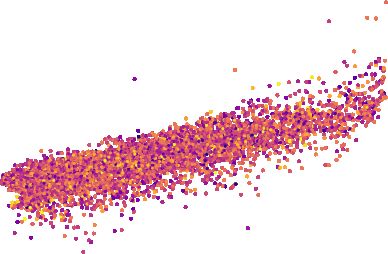
Andrae, Fouesneau, Creevey et al.: Gaia DR2: first stellar parameters from Apsis
2.0 (a) gold: 60235 2.0 (b) 2.0 (c)
silver: 10562
WDs: 481
1.5 1.5 1.5
GBP GRP [mag]
G GRP [mag]
GBP G [mag]
1.0 1.0 1.0
0.5 0.5 0.5
0.0 0.0 0.0
0.5 0.5 0.5
4000 8000 16000 32000 4000 8000 16000 32000 4000 8000 16000 32000
literature Teff [K] literature Teff [K] literature Teff [K]
Fig. 3. Colour–temperature relations for Gaia data (our reference sample described in sect. 3.2) with literature estimates of T eff . Each panel shows
a different Gaia colour. Sources with gold-standard photometry are shown in orange and those with silver-standard photometry are shown in grey.
White dwarfs matched to Kleinman et al. (2013) are shown in black.
12000
APOGEE (6049)
1.5 11000 1400 Kepler (14094)
LAMOST (5619)
1200 RAVE (2408)
10000
number of stars CU6 (4521)
literature Teff [K]
1.0 1000
G GRP [mag]
9000
8000 800
0.5 600
7000
400
6000
0.0 200
5000
0
4000 4000 5000 6000 7000 8000 9000
0.5
0.0 0.5 1.0 1.5 2.0 2.5
literature Teff [K]
GBP G [mag] Fig. 5. Distribution of literature estimates of T eff for the selected train-
ing sample. The numbers in parenthesis indicate how many stars from
Fig. 4. Colour–colour diagram for Gaia data (our reference sample de- each catalogue have been used. The test sample distribution is almost
scribed in sect. 3.2) with literature estimates of T eff . Grey lines show identical.
quality cuts where bad photometry is flagged (see Table B.1). Sources
with excess flux larger than 5 have been discarded.
This is not due to the measurement errors on fluxes, as the for-
mal uncertainties in Fig. 4 are smaller than dot size for 99% of
it is a property of ExtraTrees that this averaging should corre-
the stars plotted. Instead, this larger scatter reflects a genuine as-
spondingly reduce the bias in our results. Such a mixture is nec-
trophysical diversity that is not accounted for in the models (for
essary, because no single catalogue covers all physical parame-
example due to metallicity variations, whereas Fig. 2 is restricted
ter space with a sufficiently large number of stars for adequate
to [Fe/H] = 0).
training. Even with this mix of catalogues we had to restrict the
temperature range to 3000K−10 000K, since there are too few
literature estimates outside of this range to enable us to get good 3.3. Line-of-sight extinctions
results. For instance, there are only a few hundred OB stars with
published T eff estimates (Ramírez-Agudelo et al. 2017; Simón- For the first time, Gaia DR2 provides a colour–magnitude di-
Díaz et al. 2017). We tried to extend the upper temperature limit agram for hundreds of millions of stars with good parallaxes.
by training on white dwarfs with T eff estimates from Kleinman We complement this with estimates of the G-band extinction
et al. (2013), but as Fig. 3 reveals, the colour-temperature re- AG and the E(BP − RP) reddening such that a dust-corrected
lations of white dwarfs (black points) differ significantly from colour-magnitude diagram can be produced.
those of OB stars (orange points with T eff & 15 000K). Since As expected, we were unable to estimate the line-of-sight
ExtraTrees cannot extrapolate, this implies that stars with true extinction from just the colours, since the colour is strongly in-
T eff < 3000K or T eff > 10 000K are “thrown back” into the inter- fluenced by T eff (Fig. 2a vs. b). We therefore use the parallax
val 3000K–10 000K (see section 6.3). This may generate pecu- $ to estimate the distance and then use equation (2) to compute
liar patterns when, for example, plotting a Hertzsprung–Russell MX + AX for all three bands (which isn’t directly measured, but
diagram (see section 5.2). for convenience we refer to it from now on as an observable). We
The colour–colour diagram shown in Fig. 4 exhibits sub- then use the three observables MG + AG , MBP + ABP , MRP + ARP
stantially larger scatter than expected from the PARSEC models as features for training ExtraTrees. As shown in Fig. 6b, there
shown in Fig. 2, even inside the selected good-quality region. is a clear extinction trend in this observable space, whereas the
Article number, page 5 of 29page.29
A&A proofs: manuscript no. GDR2_Apsis
15 (a) 15 (b) 3.0 to have [Fe/H] ∼ 0. The extinctions AG , ABP , ARP and the red-
GRP + 5 log10 + 5 [mag]
GRP + 5 log10 + 5 [mag]
9000
10 10 2.5 dening E(BP−RP) = ABP −ARP are then computed for each star by
8000
2.0 subtracting from the extincted magnitudes the unextincted mag-
AG [mag]
5 7000 5
Teff [K]
6000 1.5 nitudes (which are obtained for A0 = 0 mag). We used the sam-
0 0
5000 1.0 pling of the PARSEC evolutionary models as is, without further
5 5 rebalancing or interpolation. Since this sampling is optimised
4000 0.5
10 10 0.0 to catch the pace of stellar evolution with time, the underly-
10 5 0 5 10 15 20 10 5 0 5 10 15 20
GBP + 5 log10 + 5 [mag] GBP + 5 log10 + 5 [mag] ing distribution of temperatures, masses, ages, and extinctions
is not representative of the Gaia sample. Therefore, as for T eff ,
Fig. 6. Predicted relations between observables GBP + 5 log10 $ + 5 = this will have an impact on our extinction estimates. However,
MBP + ABP and GRP + 5 log10 $ + 5 = MRP + ARP using synthetic pho- while the Gaia colours are highly sensitive to T eff , the photome-
tometry including extinction. try alone hardly allows us to constrain extinction and reddening,
such that we expect that artefacts from this mismatch of the dis-
tributions in training data and real data will be washed out by
1.75 (a) (b)
PARSEC E(BP RP) [mag]
random noise.
5 We use two separate ExtraTrees models, one for AG and one
PARSEC MG [mag]
1.50
for E(BP−RP). The input observables are MG + AG , MBP + ABP ,
1.25 0 and MRP + ARP in both cases. That is, we do not infer E(BP −
1.00 RP) from colour measurements. On account of the extinction
5
0.75 law, E(BP − RP) and AG are strongly correlated to the relation
0.50 10 AG ∼ 2 · E(BP−RP) over most of our adopted temperature range,
0.25 as can be seen in Fig. 7.8 The finite scatter is due to the different
0.00 15 spectral energy distributions of the stars: the largest deviations
0.0 0.5 1.0 1.5 2.0 2.5 3.0 3.5 0 1 2 3 4 occur for very red sources. Note that because ExtraTrees can-
PARSEC AG [mag] PARSEC GBP GRP [mag] not extrapolate beyond the training data range, we avoid negative
Fig. 7. Approximate relation between AG and E(BP−RP) (labels of Ex- estimates of AG and E(BP−RP). This non-negativity means the
traTrees training data) for PARSEC 1.2S models (Bressan et al. 2012) likelihood cannot be Gaussian, and as discussed in appendix E,
with 0 ≤ AG ≤ 4 and 3000 K≤ T eff ≤10 000 K. PARSEC models use the a truncated Gaussian is more appropriate.
extinction law of Cardelli et al. (1989). We see in panel (a) that most Evidently, the mismatch between synthetic and real Gaia
stars follow the relation AG ∼ 2 · E(BP−RP) (dashed orange line) while photometry, i.e. differences between passbands used in the train-
the stars highlighted in red behave differently. Panel (b) shows that these ing and the true passbands (and zeropoints), will have a detri-
star with different AG -E(BP−RP) relation are very red (i.e. cool) sources. mental impact on our extinction estimates, possibly leading to
systematic errors. Nonetheless, this mismatch is only ∼0.1mag
in the zeropoints (Evans et al. 2018) and as shown in Gaia Col-
dependence on T eff (Fig. 6a) is much less pronounced than in laboration et al. (2018a), the synthetic photometry (using inflight
colour-colour space (Fig. 2a). Yet, extinction and temperature passbands) of isochrone models actually agrees quite well with
are still very degenerate in some parts of the parameter space, the Gaia data. Indeed, as will be shown in sections 5.2 and 6.6,
and also there is no unique mapping of MX + AX to extinction this mismatch appears not to lead to obvious systematic errors.9
thus leading to further degeneracies (see section 6.5). Depen- Although we cannot estimate temperatures from these mod-
dence on the parallax here restricts us to stars with precise par- els with our data, the adopted T eff range of 2500–20 000 K for
allaxes, but we want to estimate AG and E(BP−RP) in order to the PARSEC models allows us to obtain reliable extinction and
correct the colour-magnitude diagram (CMD), which itself is al- reddening estimates for intrinsically very blue sources such as
ready limited by parallax precision. We do not propagate the flux OB stars, even though the method described in section 3.2 can-
and parallax uncertainties through ExtraTrees.6 not provide good T eff estimates for them.
In order to estimate extinction we cannot train our models on
literature values, for two reasons. First, there are very few reli- 4. FLAME
able literature estimate of the extinction. Second, published esti-
mates are of AV and/or E(B − V) rather than AG and E(BP−RP). The Final Luminosity, Age, and Mass Estimator (FLAME) mod-
We therefore use the PARSEC 1.2S models7 to obtain integrated ule aims to infer fundamental parameters of stars. In Gaia DR2
photometry from the synthetic Atlas 9 spectral libraries (Castelli we only activate the components for inferring luminosity and
& Kurucz 2003) and the nominal instrument passbands (Fig. 1). radius. Mass and age will follow in the next data release, once
These models use the extinction law from Cardelli et al. (1989) GSP-Phot is able to estimate log g and [Fe/H] from the BP/RP
and O’Donnell (1994) with a fixed relative extinction parameter, spectra and the precision in T eff and AG improves. We calculate
R0 =3.1. We constructed a model grid that spans A0 = 0–4 mag, a luminosity L with
temperature range of 2 500–20 000 K, a log g range of 1–6.5 dex,
and a fixed solar metallicity (Z = 0.0152, [Fe/H] = 0). We −2.5 log10 L = MG + BCG (T eff ) − Mbol (4)
chose solar metallicity for our models since we could not cover where L is in units of L (Table 3), MG is the absolute mag-
all metallicities and because we expect most stars in our sample nitude of the star in the G-band, BCG (T eff ) is a temperature
6 8
We found that propagating the flux and parallax uncertainties through Using different stellar atmosphere models with different underlying
the ExtraTrees has no noteworthy impact on our results, i.e. our extinc- synthetic SEDs, Jordi et al. (2010) found a slightly different relation
tion and reddening estimates are not limited by the expected precision between AG and E(BP−RP).
of the input data. 9
The situation for T eff would be different, where using synthetic
7
http://stev.oapd.inaf.it/cgi-bin/cmd colours results in large errors.
Article number, page 6 of 29page.29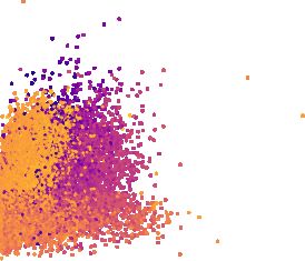
Andrae, Fouesneau, Creevey et al.: Gaia DR2: first stellar parameters from Apsis

Table 3. Reference solar parameters.

                   quantity            unit value                                            0.0
                        R                m      6.957e+08
                      T eff              K      5.772e+03
                                                                                             0.5

                                                                                 BCG [mag]
                        L               W       3.828e+26
                     Mbol              mag      4.74
                     BCG               mag    +0.06                                          1.0
                        V              mag −26.76
                     BCV               mag    −0.07
                      MV               mag      4.81                                         1.5

                                                                                             2.0
dependent bolometric correction (defined below), and Mbol =                                     8000          7000          6000       5000       4000
4.74 mag is the solar bolometric magnitude as defined in IAU                                                                  Teff [K]
Resolution 2015 B210 . The absolute magnitude is computed
from the G-band flux and parallax using equations 1 and 2. As                     Fig. 8. Bolometric corrections from the MARCS models (grey dots) and
the estimates of extinction provided by Priam were shown not                      the subset we selected (open circles) to fit the polynomial model (equa-
                                                                                  tion 7, with fixed a0 ), to produce the thick blue line and the associated
to be sufficiently accurate on a star-to-star basis for many of our               1-σ uncertainty indicated by the blue shaded region.
brighter validation targets, we set AG to zero when computing
MG . The radius R is then calculated from equation 3 using this
luminosity and T eff from Priam. These derivations are somewhat
                                                                                  still a dependence on log g, we adopt for each T eff bin the mean
trivial; at this stage FLAME simply provides easy access for the
                                                                                  value of the bolometric correction. We also compute the stan-
community to these fundamental parameters.
                                                                                  dard deviation σ(BCG ) as a measure of the uncertainty due to
    Should a user want to estimate luminosity or radius assuming
                                                                                  the dispersion in log g. We then fit a polynomial to these values
a non-zero extinction AG,new and/or a change in the bolometric
                                                                                  to define the function
correction of ∆BCG , one can use the following expressions
                                                                                                   4
Lnew = L 100.4(AG,new −∆BCG )
                                                                                                   X
                                                                           (5)    BCG (T eff ) =         ai (T eff − T eff )i .                             (7)
                                                                                                   i=0
Rnew = R 10   0.2(AG,new −∆BCG )
                                   .                                       (6)
                                                                                  The values of the fitted coefficients are given in Table 4. The fit
                                                                                  is actually done with the offset parameter a0 fixed to BCG =
4.1. Bolometric Correction                                                        +0.06 mag, the reference bolometric value of the Sun (see ap-
                                                                                  pendix D). We furthermore make two independent fits, one for
We obtained the bolometric correction BCG on a grid as a func-                    the T eff in the range 4000–8000 K and another for the range
tion of T eff , log g, [M/H], and [α/Fe], derived from the MARCS                  3300–4000 K.
synthetic stellar spectra (Gustafsson et al. 2008). The synthetic
spectra cover a T eff range from 2500K to 8000K, log g from                       Table 4. Polynomial coefficients of the model BCG (T eff ) defined in
−0.5 to 5.5 dex, [Fe/H] from −5.0 to +1.0 dex, and [α/Fe] from                    equation 7 (column labelled BCG ). A separate model was fit to the two
+0.0 to +0.4 dex. Magnitudes are computed from the grid spec-                     temperature ranges. The coefficient a0 was fixed to its value for the
tra using the G filter (Fig. 1). These models assume local ther-                  4000–8000 K temperature range. For the lower temperature range a0
modynamic equilibrium (LTE), with plane-parallel geometry for                     was fixed to ensure continuity at 4000 K. The column labelled σ(BCG )
dwarfs and spherical symmetry for giants. We extended the T eff                   lists the coefficients for a model of the uncertainty due to the scatter of
range using the BCG from Jordi et al. (2010), but with an offset                  log g.
added to achieve continuity with the MARCS models at 8000
K. However, following the validation of our results (discussed                                                       BCG       σ(BCG )
later), we choose to filter out FLAME results for stars with T eff                                                 4000 – 8000 K
outside the range 3300 – 8000 K (see appendix A).                                                        a0    6.000e−02    2.634e−02
    For the present work we had to address two issues. First, BCG                                        a1    6.731e−05    2.438e−05
is a function of four stellar parameters, but it was necessary to                                        a2   −6.647e−08 −1.129e−09
project this to be a function of just T eff , since for Gaia DR2 we                                      a3    2.859e−11 −6.722e−12
do not yet have estimates of the other three stellar parameters.                                         a4   −7.197e−15    1.635e−15
Second, the bolometric correction needs a reference point to set                                                   3300 – 4000 K
the absolute scale, as this is not defined by the models. We will                                        a0    1.749e+00 −2.487e+00
refer to this as the offset of the bolometric correction, and it has                                     a1    1.977e−03 −1.876e−03
been defined here so that the solar bolometric correction BCG                                            a2    3.737e−07    2.128e−07
is +0.06 mag. Further details are provided in appendix D.                                                a3   −8.966e−11    3.807e−10
    To provide a 1-D bolometric correction, we set [α/Fe]=0 and                                          a4   −4.183e−14    6.570e−14
select the BCG corresponding11 to |[Fe/H]| < 0.5. As there is
10
   https://www.iau.org/static/resolutions/IAU2015_
English.pdf
11
   Choosing |[Fe/H]| < 1.0 or including [α/Fe] = +0.4 only changed                ing [Fe/H] to a single value (e.g. zero) had just as little impact relative
the BCG in the third decimal place, well below its final uncertainty. Fix-        to the uncertainty.

                                                                                                                             Article number, page 7 of 29page.29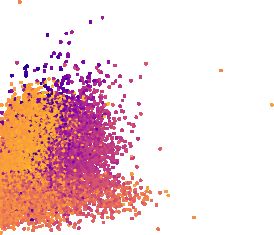
A&A proofs: manuscript no. GDR2_Apsis

    Fig. 8 shows BCG as a function of T eff . The largest uncer-                                     0.200
tainty is found for T eff < 4000 K where the spread in the values                                    0.175
                                                                                                                 (a)
can reach up to ±0.3 mag, due to not distinguishing between gi-                                      0.150

                                                                              relative uncertainty
ants and dwarfs12 . We estimated the uncertainty in the bolomet-                                     0.125
ric correction by modelling the scatter due to log g as a function                                   0.100
of T eff , using the same polynomial model as in equation 7. The                                     0.075
coefficients for this model are also listed in Table 4.
                                                                                                     0.050
                                                                                                     0.025
4.2. Uncertainty estimates on luminosity and radius                                                  0.000
                                                                                                                       100             101                         102               103
The upper and lower uncertainty levels for L are defined sym-                                                                           radius [         ]
metrically as L±σ, where σ has been calculated using a standard                                           0.35
(first order) propagation of the uncertainties in the G-band mag-                                                (b)
                                                                                                          0.30
nitude and parallax13 . Note, however, that we do not include the

                                                                                   relative uncertainty
additional uncertainty arising from the temperature which would                                           0.25
propagate through the bolometric correction (equation 4). For R,                                          0.20
the upper and lower uncertainty levels correspond to the radius                                           0.15
computed using the upper and lower uncertainty levels for T eff .
As these T eff levels are 16th and 84th percentiles of a distribu-                                        0.10

tion, and percentiles are conserved under monotonic transforma-                                           0.05
tions of distributions, the resulting radius uncertainty levels are                                       0.00
also the 16th and 84th percentiles. This transformation neglects                                                       10   1   100   101          102           103     104   105
                                                                                                                                      luminosity [           ]
the luminosity uncertainty, but in most cases the T eff uncertainty
dominates for the stars in the published catalogue (i.e. filtered              Fig. 9. Distribution of FLAME relative uncertainties for (a) radius and
results; see Appendix A). The distribution of the uncertainties in             (b) luminosity, after applying the GDR2 filtering (Table A.1). In both
R and L for different parameter ranges are shown as histograms                 panels the black line shows the median value of the uncertainty, and the
in Figs. 9. The radius uncertainty defined here is half the differ-            shaded regions indicate the 16th and 84th percentiles.
ence between the upper and lower uncertainty levels. It can be
seen that the median uncertainties in L, which considers just the
uncertainties in G and $, is around 15%. For radius it’s typically             on this test set. The smallest lower uncertainty level is 3098 K
less than 10%. While our uncertainty estimates are not particu-                and the highest upper uncertainty level is 9985 K. As the uncer-
larly precise, they provide the user with some estimate of the                 tainties are percentiles of the distribution of ExtraTrees outputs,
quality of the parameter.                                                      and this algorithm cannot extrapolate, these are constrained to
                                                                               the range of our training data (which is 3030 K to 9990 K).
5. Results and catalogue content
                                                                               Table 5. T eff error on various sets of test data for sources which were not
We now present the Apsis results in Gaia DR2 by looking at the                 used in training. We also show test results for 8599 sources with clean
performance on various test data sets. We refer to summaries of                flags from the GALAH catalogue (Martell et al. 2017), a catalogue not
the differences between our results and their literature values as             used in training at all. The bias is the mean error.
“errors”, as by design our algorithms are trained to achieve min-
imum differences for the test data. This does not mean that the                                              reference catalogue             bias [K] RMS error [K]
literature estimates are “true” in any absolute sense. We ignore                                             APOGEE                             −105            383
here the inevitable inconsistencies in the literature values, since                                          Kepler Input Catalogue                −6           232
we do not expect our estimates to be good enough to be substan-                                              LAMOST                                −9           381
tially limited by these.                                                                                     RAVE                                  21           216
                                                                                                             RVS Auxiliary Catalogue             −50            425
5.1. Results for T eff                                                                                       GALAH                               −18            233

We use the test data set (as defined in section 3.2) to examine the
quality of our T eff estimates. We limit our analyses to those 98%
of sources which have “clean” Priam flags for T eff (defined in                    Fig. 10 compares our T eff estimates with the literature esti-
appendix B). Our estimated values range from 3229 K to 9803 K                  mates for our test data set. The root-mean-squared (RMS) test
                                                                               error is 324 K, which includes a bias (defined as the mean resid-
12
   We could have estimated a mass from luminosities and colours in or-         ual) of −29 K. For comparison, the RMS error on the training
der to estimate log g, and subsequently iterated to derive new luminosi-       set is 217 K, with a bias of −22 K (better than the test set, as
ties and radii. However, given the uncertainties in our stellar parameters,    expected). We emphasise that the RMS test error of 324 K is an
we decided against doing this.                                                 average value over the different catalogues, which could have
13
   A revision of the parallax uncertainties between processing and the         different physical T eff scales. Moreover, since our test sample,
data release means that our fractional luminosity uncertainties are incor-
                                                                               just like our training sample, is not representative for the general
rect by factors varying between 0.6 and 2 (for 90% of the stars), with
some dependence on magnitude (see appendix A of Lindegren et al.               stellar population in Gaia DR2, the 324 K uncertainty estimate is
(2018), in particular the upper panel of Figure A.2). Although there was       likely to be an underestimate. Nevertheless, given this RMS test
no opportunity to rederive the luminosity uncertainties, these revised         error of 324 K, we can subtract (in quadrature) the 102 K litera-
parallax uncertainties (i.e. those in Gaia DR2) were used when filtering       ture uncertainty (Table 2) to obtain an internal test error estimate
the FLAME results according to the criterion in appendix A.                    of 309 K for Priam.
Article number, page 8 of 29page.29
Andrae, Fouesneau, Creevey et al.: Gaia DR2: first stellar parameters from Apsis
(a) bias: -29K (a) 15 (b)
relative test error [%]
800
RMSE: 324K 600 10
test error [K]
9000
400
5
200
8000 0
0
Priam Teff [K]
200 5
7000 4000 5000 6000 7000 8000 9000 4000 5000 6000 7000 8000 9000
Priam Teff [K] Priam Teff [K]
6000 800 (c) 600 (d)
600 400
test error [K]
test error [K]
5000
APOGEE 400 200
Kepler 200 0
LAMOST 0 200
4000
RAVE 200 400
CU6 4000 5000 6000 7000 8000 9000 4 6 8 10 12 14 16
3000 literature Teff [K] G [mag]
750 (b)
3000
4000
5000
6000
7000
8000
9000
600 (e) 600 (f)
500
400 400
test error [K]
test error [K]
250
Teff [K]
0 200 200
250 0 0
500 200 200
750
400 400
3000 4000 5000 6000 7000 8000 9000 0.5 1.0
1.5 2.0 2.5 0.0 0.5 1.0 1.5 2.0 2.5 3.0 3.5
literature Teff [K] Priam AG [mag] GBP GRP [mag]
Fig. 10. Comparison of Priam T eff estimates with literature values on Fig. 11. Dependence of T eff test errors on estimated T eff (panel a and
the test data set for sources with clean flags, colour coded according relative errors in panel b), on literature T eff (panel c), on G (panel
to catalogue. The upper panel plots the Priam outputs; the lower panel d), estimated AG (panel e) and GBP − GRP colour (panel f). Red lines
plots the residuals ∆T eff = T eff
Priam literature
− T eff . shows root-mean-squared errors (dashed) and root-median-squared er-
rors (solid). Blue lines show mean errors (dashed) and median errors
(solid), as measures of bias.
Table 5 shows that the errors vary considerably for the differ- 75° 400
ent reference catalogues. Consequently, the temperature errors 60°
for a stellar population with a restricted range of T eff could differ 45° 300
30° 200
Galactic b [deg]
from our global estimates (see sections 6.3 and 6.4). This is illus-
trated in panels (a) and (b) of Fig. 11. If the estimated tempera- 15° 100
150 120 90 60 30 0 -30 -60 -90 -120 -150
Teff [K]
ture is below about 4000 K, we can expect errors of up to 550 K. 0° 0
Likewise, if the estimated temperature is above 8000 K, the abso- -15° 100
lute error increases while the relative error is consistently below -30° 200
10% for T eff & 4 000 K. The dependence of test error on litera- -45° 300
ture temperatures (Fig. 11c) shows the same behaviour. Note that -60°
-75° 400
the errors are dominated by outliers, since when we replace the Galactic [deg]
mean by the median, the errors are much lower (solid vs. dashed
Fig. 12. Mean difference of Priam T eff from literature values for test
lines in Fig. 11). data, plotted in Galactic coordinates (Mollweide projection).
As we can see from Fig. 11d, the temperature error increases
only very slightly with G magnitude, which is best seen in the
medians since outliers can wash out this trend in the means.
Fig. 11e shows that the temperature error is weakly correlated of 10 000 K in the training sample (but not in the Galaxy) and
with the estimated AG extinction, but now more dominant in the the inability of ExtraTrees to extrapolate.
mean than the median. This is to be expected since our train- Fig. 12 also suggests a slight tendency to systematically
ing data are mostly stars with low extinctions. Stars with high overestimate T eff at high Galactic latitudes. Halo stars typically
extinctions are under-represented, and due to the extinction– have subsolar metallicity, hence tend to be bluer for a given
temperature degeneracy they are assigned systematically lower T eff than solar metallicity stars. This may lead Priam, which is
T eff estimates. This is particularly apparent when we plot the trained mostly on solar-metallicity stars, to overestimate T eff (see
temperature residuals in the Galactic coordinates (Fig. 12): stars Sect. 6.1). Alternatively, although the extinction in our empirical
in the Galactic plane, where extinctions are higher, have system- training sample is generally low, it is not zero, such that for high
atically negative residuals. Finally, Fig. 11f shows that the tem- latitude stars with almost zero extinction, Priam would overes-
perature error also depends on the GBP − GRP colour of the star. timate T eff . Most likely, both effects are at work, with the latter
Very blue and very red stars were comparatively rare in the train- presumably dominating.
ing data. For the bluest stars, we see that we systematically un- The differences between our temperature estimates and the
derestimate T eff . This is a direct consequence of the upper limit literature values are shown in a CMD in Fig. 13a. Priam predicts
Article number, page 9 of 29page.29A&A proofs: manuscript no. GDR2_Apsis
10
(a) (b) 90 180
10
400 = 0.81 = 0.06
300
= 1.20 = 1.04
N = 291 N = 1404
G + 5 log10( ) + 5 [mag]
5 80 140
= 0.80 = 0.14
5
200
= 1.11 = 1.14
100 N = 617 N = 1317
0 70 = 0.71 100 = 0.28
Teff [K]
0
0 = 0.99 = 1.06
N = 815 N = 1316
100 60 60
Galactic Latitude |b|
5 = 0.76 = 0.17
Galactic Longitude
= 1.41
5
200 = 1.04
N = 1183 N = 2494
300 50 = 0.45 20 = 0.12
10
= 1.00 = 1.41
10
400 N = 1538 N = 3239
0 1 2 3 4 10000 9000 8000 7000 6000 5000 4000 3000 40 = 0.41 20 = 0.13
GBP GRP [mag] Priam Teff [K] = 1.02 = 1.35
N = 2161 N = 1448
30 = 0.17 60 = 0.00
Fig. 13. Difference between Priam T eff and literature values for the test
= 1.03 = 0.74
data shown in a colour-magnitude diagram (left panel) and Hertzsprung- N = 2361 N = 4612
20 = 0.00 100 = 0.00
Russell diagram (right panel). = 0.66 = 0.69
N = 15817 N = 16100
10 = 0.30 140 = 0.16
= 0.99 = 1.48
N = 9032 N = 1885
0 180
lower T eff in those parts of the CMD where we suspect the ex- 4 2 0 2 4 4 2 0 2 4
Teff, Priam Teff, Lit Teff, Priam Teff, Lit
tinction may be high (e.g. the lower part of the giant branch). lit + Priam
2 2
lit + Priam
2 2
Conversely, the overestimation of T eff in the lower part of the
main sequence may be due nearby faint stars having lower ex- Fig. 14. Distribution of the T eff residuals (Priam minus literature) nor-
tinctions than the low but non-zero extinction in our empirical malized by their combined uncertainties for the test data set, for differ-
training sample. These systematics with extinction agree with ent Galactic latitudes (left column) and longitudes (right column). The
Fig. 11e. This will be discussed further in the next section. Priam uncertainty σPriam used in the computation for each star is formed
In order to assess our uncertainty estimates, we again use from the lower uncertainty level if T eff,Priam > T eff,lit , and from the upper
uncertainty level otherwise. The upper left corner of each panel reports
the test data. Ideally, the distribution of our uncertainty esti- the mean µ and standard deviation (σ) of these normalized residuals.
mates should coincide with the distribution of the errors. We find The red curves are unit Gaussian distributions. The vertical lines indi-
that for 23% of test stars, their literature values are below our cate the median of each distribution. For unbiased estimates and correct
lower uncertainty levels (which are 16th percentiles), whereas uncertainties in both the literature and our work, the histograms and the
for 22% of test stars the literature values are above our upper red Gaussians should match.
uncertainty levels (84th percentiles). One interpretation of this
is that our uncertainty intervals are too narrow, i.e. that the sup-
posed 68% central confidence interval (84th minus 16th) is in
fact more like a 55% confidence interval. However, the literature 5.2. Results for AG and E(BP−RP)
estimates have finite errors, perhaps of order 100–200 K, and
We look now at our estimates of line-of-sight extinction AG and
these will increase the width of the residual distribution (com-
reddening E(BP−RP). Where appropriate we will select on paral-
pared to computing residuals using perfect estimates). We inves-
lax uncertainty. As will be discussed in section 6.5, some of our
tigate this more closely by plotting the distribution of residuals
estimates of AG and E(BP−RP) suffered from strong degenera-
normalised by the combined (Priam and literature) uncertainty
cies. These (about one third of the initial set of estimates) were
estimates. This is shown in Fig. 14 for all our test data and differ-
filtered out of the final catalogue.
ent directions in the Galaxy. If the combined uncertainties were
Gaussian measures of the residuals, then the histograms should As explained in section 3.3, we are unable to estimate the
be Gaussian with zero mean and unit standard deviation (the red line-of-sight extinction from just the colours. Fig. 15 demon-
curves). This is generally the case, and suggests that, although strates that neither AG nor E(BP−RP) has a one-to-one relation
we do not propagate the flux uncertainties, the Priam uncertainty with the colour. (Plots against the other two colours are shown in
estimates may indeed provide 68% confidence intervals and that the online Gaia DR2 documentation.) This complex distribution
the 55% obtained above arose only from neglecting literature un- is the combined result of having both very broad filters and a
certainties. The left column in Fig. 14 shows a systematic trend wide range of stellar types. It may be possible to find an approx-
in the residuals (mean of the histogram) as a function of Galactic imative colour–extinction relation only if one can a priori restrict
latitude, which is also evident from Fig. 12. This most likely re- the sample to a narrow part of the HRD, such as giant stars.
flects a systematic overestimation of T eff for zero-extinction stars In addition, using only three optical bands (and parallax),
at high latitudes. Also note that the panels for ` = 60◦ − 100◦ and we do not expect very accurate extinction estimates. A direct
|b| = 10◦ − 20◦ exhibit narrow peaks. These two panels are dom- comparison to the literature is complicated by the fact that the
inated by the Kepler field, which makes up 43% of the training literature does not estimate AG or E(BP − RP) but rather A0 ,
sample (see Table 2). The fact that these two peaks are sharper AV , or E(B − V). We compare them nonetheless on a star-by-
than the unit Gaussian suggests overfitting of stars from the Ke- star basis in Table 6, and Fig. 16 shows the results for stars for
pler sample.14 Concerning the asymmetry of the conference in- the Kepler Input Catalog. The largest RMS difference for these
tervals, we find that for 57% of sources, upper minus median and samples is 0.34 mag between AG and AV and 0.24 mag between
median minus lower differ by less than a factor of two, while for E(BP−RP) and E(B−V). This appears to be dominated primarily
2.5% of sources these two bands can differ by more than a factor by systematically larger values of AG and E(BP−RP). The dif-
of ten. ferences between nominal and real passbands are only of order
0.1 mag in the zeropoints (Evans et al. 2018) and thus are un-
14
Propagating the flux errors through the ExtraTrees gives slightly likely to explain this. Instead, these large values arise from the
lower test errors (supporting the idea that we may overfit the Kepler degeneracies in the extinction estimation (see section 6.5) and
sample) and brings the normalised residuals closer to a unit Gaussian. the non-trivial transformation between AV and AG and between
Article number, page 10 of 29page.29You can also read