Simulation and Analysis of the Operation and Reconfiguration of a Medium Voltage Distribution Network in a Smart Grid Context in MATLAB Simulink ...
←
→
Page content transcription
If your browser does not render page correctly, please read the page content below

Simulation and Analysis of the Operation
and Reconfiguration of a Medium Voltage
Distribution Network in a Smart Grid
Context in MATLAB Simulink

ALEXANDER VAN WAEYENBERGE
Junho de 2021
Instituto Superior de Engenharia do Porto
             Departamento de Engenharia Electrotécnica
     Rua Dr. António Bernardino de Almeida, 431, 4249-015 Porto

 Simulation and Analysis of the
Operation and Reconfiguration of
 a Medium Voltage Distribution
Network in a Smart Grid Context
     in MATLAB Simulink

  Mestrado em Engenharia Eletrotécnica - Sistemas Elétricos de Energia

                Alexander Van Waeyenberge

                               Supervisors:
                  Dr. Bruno Miguel Da Rocha Canizes
                      Dr. João André Pinto Soares
                           Dr. Simon Ravyts

                         Ano Letivo: 2020-2021
Abstract

This work will present a Medium Voltage Distribution Network that is operated
as a Smart Grid. As the distribution infrastructure for electric energy ages and
the share of EV’s and renewables increases, changes will have to be made to sup-
port the increasing power flows in the network. A more long-term solution than
reinforcing the network with heavier cables is constructing an intelligent network
that reacts to changing power flows inside the network and adapts accordingly to
guarantee optimal functionality. External data from an optimisation algorithm is
used to determine the switching behaviour. The network was modeled and anal-
ysed using a simulation software. If done correctly, a simulation can offer a lot
of insight for only a fraction of the cost of constructing and testing the network
in reality. MATLAB Simulink was used for the virtual modeling and analysis
of the network. The main objective is to construct a model of the MVDN and
use it to generate and analyse the power flows in the network to determine the
plausibility of exploiting a similar network in an existing city. The models for
each of the network components were developed and picked to combine them into
a functioning network model based on the smart city’s topology. Simulating a
smart grid is in essence not novel, but has not been done in Simulink before in
this context. The hardest obstacle to overcome during the construction of the
network model was finding a way to achieve the making and breaking of network
connections in a way that Simulink could compute the network parameters cor-
rectly and in a timely manner. A whole section is dedicated to resolving these
development issues. Following this, the results of the simulation regarding power
flows and losses in the network are discussed. When it comes to the renewable
generation implementation, the results showed promising results, even on days
with low wind velocity the renewables aided in reducing the power demanded
from the substation. The total generated power is compared with the total con-
sumed power in the loads to find the grid losses. It became apparent very quickly
that the grid losses were very high, up to 9.7%, which is a lot higher than the
expected 2-6%. Overall the model showed promising results, as well as serving
as a baseline for future works to improve upon.

                                        iii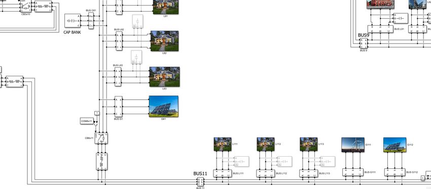
Contents

Contents                                                                                                                                   i

List of Figures                                                                                                                           v

List of Tables                                                                                                                           vii

Glossary                                                                                                                                 ix

Acknowledgements                                                                                                                         xi

1   Introduction                                                                                                                          1
    1.1 Problem . . . .    . . . .   .   .   .   .   .   .   .   .   .   .   .   .   .   .   .   .   .   .   .   .   .   .   .   .   .    1
    1.2 Motivation . .     . . . .   .   .   .   .   .   .   .   .   .   .   .   .   .   .   .   .   .   .   .   .   .   .   .   .   .    2
    1.3 Objectives . . .   . . . .   .   .   .   .   .   .   .   .   .   .   .   .   .   .   .   .   .   .   .   .   .   .   .   .   .    2
    1.4 Requirements .     . . . .   .   .   .   .   .   .   .   .   .   .   .   .   .   .   .   .   .   .   .   .   .   .   .   .   .    4
    1.5 Structure of the   Thesis    .   .   .   .   .   .   .   .   .   .   .   .   .   .   .   .   .   .   .   .   .   .   .   .   .    4

2   Medium Voltage Distribution Network                      in a Smart Grid Context                                                      5
    2.1 Distribution lines . . . . . . . . .                 . . . . . . . . . . . . . . .                               .   .   .   .    6
        2.1.1 Transmission line theory .                     . . . . . . . . . . . . . . .                               .   .   .   .    7
    2.2 Substations . . . . . . . . . . . .                  . . . . . . . . . . . . . . .                               .   .   .   .    8
        2.2.1 Transformer construction                       . . . . . . . . . . . . . . .                               .   .   .   .    9
        2.2.2 No-load losses . . . . . . .                   . . . . . . . . . . . . . . .                               .   .   .   .   10
        2.2.3 Load losses . . . . . . . .                    . . . . . . . . . . . . . . .                               .   .   .   .   11
        2.2.4 Equivalent circuits . . . .                    . . . . . . . . . . . . . . .                               .   .   .   .   11
    2.3 Switches . . . . . . . . . . . . . .                 . . . . . . . . . . . . . . .                               .   .   .   .   13
    2.4 Capacitor banks . . . . . . . . .                    . . . . . . . . . . . . . . .                               .   .   .   .   14
    2.5 Conclusions . . . . . . . . . . . .                  . . . . . . . . . . . . . . .                               .   .   .   .   16

3   Modeling an MVDN Inside MATLAB Simulink                                     17
    3.1 Methodology . . . . . . . . . . . . . . . . . . . . . . . . . . . . . . 17

                                                     i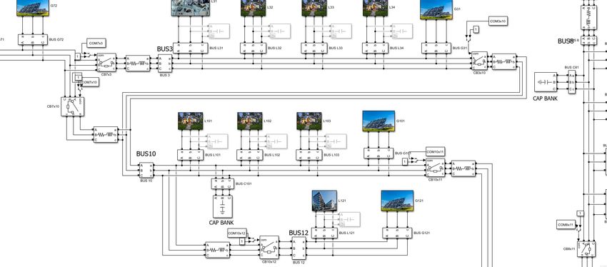
ii                                                                                               CONTENTS

     3.2   Software environment . . . . . . . . . .      .   .   .   .   .   .   .   .   .   .   .   .   .   .   .   19
     3.3   Simulation in general . . . . . . . . . . .   .   .   .   .   .   .   .   .   .   .   .   .   .   .   .   20
           3.3.1 Simulation Settings . . . . . . . .     .   .   .   .   .   .   .   .   .   .   .   .   .   .   .   20
           3.3.2 Solver . . . . . . . . . . . . . . .    .   .   .   .   .   .   .   .   .   .   .   .   .   .   .   20
                  3.3.2.1 Fixed-step solver: . . .       .   .   .   .   .   .   .   .   .   .   .   .   .   .   .   22
                  3.3.2.2 Variable-step solver . .       .   .   .   .   .   .   .   .   .   .   .   .   .   .   .   23
                  3.3.2.3 Continuous vs discrete .       .   .   .   .   .   .   .   .   .   .   .   .   .   .   .   23
                  3.3.2.4 Selected solver . . . . .      .   .   .   .   .   .   .   .   .   .   .   .   .   .   .   24
           3.3.3 Simscape and powergui . . . . .         .   .   .   .   .   .   .   .   .   .   .   .   .   .   .   25
     3.4   Simulation component models . . . . . .       .   .   .   .   .   .   .   .   .   .   .   .   .   .   .   27
           3.4.1 Distribution lines . . . . . . . . .    .   .   .   .   .   .   .   .   .   .   .   .   .   .   .   27
           3.4.2 Circuit breaker . . . . . . . . . .     .   .   .   .   .   .   .   .   .   .   .   .   .   .   .   28
           3.4.3 Substation . . . . . . . . . . . .      .   .   .   .   .   .   .   .   .   .   .   .   .   .   .   30
           3.4.4 Busbars . . . . . . . . . . . . . .     .   .   .   .   .   .   .   .   .   .   .   .   .   .   .   34
           3.4.5 Dynamic loads and generation .          .   .   .   .   .   .   .   .   .   .   .   .   .   .   .   35
           3.4.6 Capacitor banks . . . . . . . . .       .   .   .   .   .   .   .   .   .   .   .   .   .   .   .   39
           3.4.7 Simulation setup script . . . . .       .   .   .   .   .   .   .   .   .   .   .   .   .   .   .   39
           3.4.8 Conclusions . . . . . . . . . . . .     .   .   .   .   .   .   .   .   .   .   .   .   .   .   .   41

4    Results of the MVDN Simulation                                                                                  43
     4.1 Development issues . . . . . . . . . . . . . . . . . . . . . . . . . .                                  .   43
         4.1.1 The Breaker Problem . . . . . . . . . . . . . . . . . . . .                                       .   43
         4.1.2 Possible causes . . . . . . . . . . . . . . . . . . . . . . . .                                   .   46
                  4.1.2.1 Scalability issue . . . . . . . . . . . . . . . . . .                                  .   46
                  4.1.2.2 Solver settings . . . . . . . . . . . . . . . . . . .                                  .   46
                  4.1.2.3 The combination of breakers and dynamic loads                                          .   46
         4.1.3 Possible solutions . . . . . . . . . . . . . . . . . . . . . . .                                  .   47
                  4.1.3.1 Changing the breakers with variable resistors . .                                      .   47
                  4.1.3.2 Switching off the main power during the breaker
                           reconfiguration . . . . . . . . . . . . . . . . . . .                                 . 48
                  4.1.3.3 Composite block simulation . . . . . . . . . . . .                                     . 48
                  4.1.3.4 Change detecting MATLAB script . . . . . . . .                                         . 49
                  4.1.3.5 Commenting breakers in/out using a MATLAB
                           script . . . . . . . . . . . . . . . . . . . . . . . .                                .   50
     4.2 Results . . . . . . . . . . . . . . . . . . . . . . . . . . . . . . . . .                               .   51
         4.2.1 Power flows inside the MVDN . . . . . . . . . . . . . . . .                                       .   52
     4.3 Conclusion . . . . . . . . . . . . . . . . . . . . . . . . . . . . . .                                  .   61

5    Conclusions                                                                63
     5.1 Conclusions on the simulation of a MVDN in a smart grid context 63
     5.2 Suggestions and future works . . . . . . . . . . . . . . . . . . . . . 65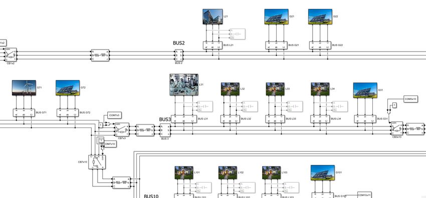
CONTENTS                                                                       iii

Bibliography                                                                  67

A Switching, Load and Generation data                                          71
  A.1 Switching data . . . . . . . . . . . . . . . . . . . . . . . . . . . . . 71
  A.2 Loads and Generation Data . . . . . . . . . . . . . . . . . . . . . . 73

B Network Model                                                               75

C Charging station example                                                    81
List of Figures
2.1 Transmission Theory Model . . . . . . . . . . . . . . . . . . . . . . . . 8
2.2 Transformer . . . . . . . . . . . . . . . . . . . . . . . . . . . . . . . . . 9
2.3 Equivalent circuit of a transformer . . . . . . . . . . . . . . . . . . . . 12
2.4 Equivalent T-circuit of a transformer referred to primary . . . . . . . 13
2.5 Resistive snubber . . . . . . . . . . . . . . . . . . . . . . . . . . . . . . 14
3.1 Methodology . . . . . . . . . . . . . . . . . . . . . . . . . . . . . . . . 18
3.2 Simulink solver flowchart . . . . . . . . . . . . . . . . . . . . . . . . . 24
3.3 Solver settings for ODE23tb . . . . . . . . . . . . . . . . . . . . . . . . 25
3.4 Distribution line differential equation . . . . . . . . . . . . . . . . . . . 28
3.5 Distribution line in Simulink . . . . . . . . . . . . . . . . . . . . . . . 28
3.6 3-Phase circuit breaker in Simulink . . . . . . . . . . . . . . . . . . . . 29
3.7 Switching setup for 3-phase breaker with respect to time . . . . . . . . 29
3.8 Substation in Simulink . . . . . . . . . . . . . . . . . . . . . . . . . . . 31
3.9 Dyn1 vector diagram . . . . . . . . . . . . . . . . . . . . . . . . . . . . 34
3.10 Busbar in Simulink . . . . . . . . . . . . . . . . . . . . . . . . . . . . . 35
3.11 Voltage, current, active & reactive power measurement . . . . . . . . . 35
3.12 Dynamic load in Simulink . . . . . . . . . . . . . . . . . . . . . . . . . 36
3.13 Dynamic generation in Simulink . . . . . . . . . . . . . . . . . . . . . 37
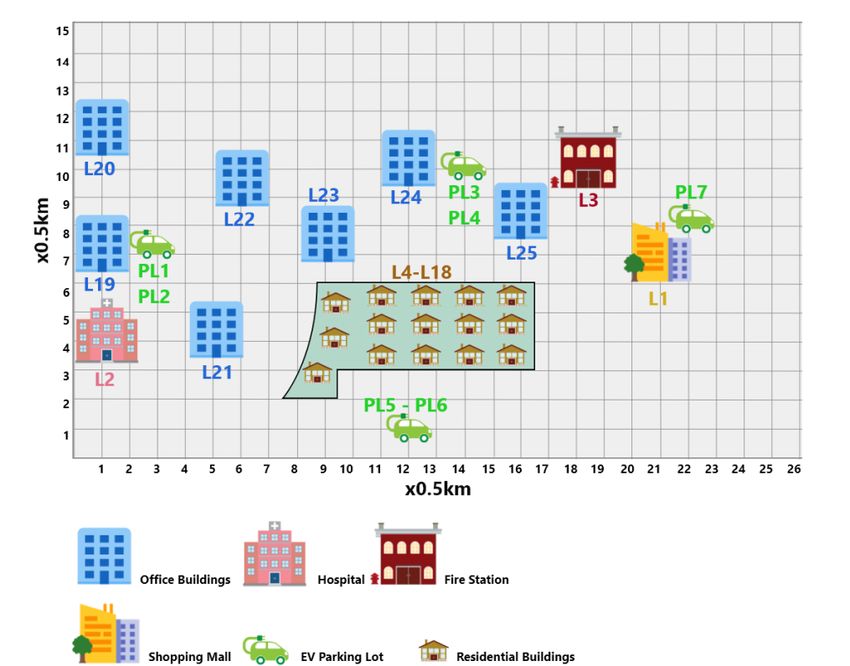
3.14 Map of the loads of the simulated smart city . . . . . . . . . . . . . . 38
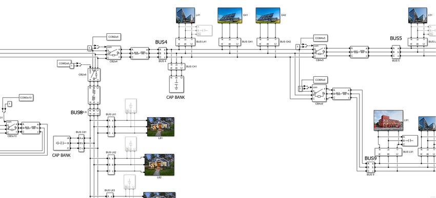
3.15 Single-wire diagram of the smart city . . . . . . . . . . . . . . . . . . . 38
3.16 Capacitor bank in Simulink . . . . . . . . . . . . . . . . . . . . . . . . 39
3.17 File loading script for active power data . . . . . . . . . . . . . . . . . 40
3.18 Initialisation variables of the simulation . . . . . . . . . . . . . . . . . 41
3.19 Flowchart of the simulation . . . . . . . . . . . . . . . . . . . . . . . . 41
4.1 Abnormal solver behaviour . . . . . . . . . . . . . . . . . . . . . . . . 45
4.2 Breaker Problem test setup . . . . . . . . . . . . . . . . . . . . . . . . 47
4.3 Variable resistor in Simulink . . . . . . . . . . . . . . . . . . . . . . . . 48
4.4 Three-phase composite blocks in simulink . . . . . . . . . . . . . . . . 49
vvi LIST OF FIGURES
4.5 Example of spikes in figure . . . . . . . . . . . . . . . . . . . . . . . . 52
4.6 Active power generated by renewable generation . . . . . . . . . . . . 53
4.7 Active power generated by the substation . . . . . . . . . . . . . . . . 54
4.8 Total Active power generated by renewable generation and substation 54
4.9 Active power consumed by the dynamic loads . . . . . . . . . . . . . . 55
4.10 Comparison between active power generated and consumed . . . . . . 56
4.11 Active power consumed by grid losses . . . . . . . . . . . . . . . . . . 56
4.12 Active power comparison between both sides of the substation . . . . 57
4.13 Reactive power consumed by the dynamic loads . . . . . . . . . . . . . 58
4.14 Reactive power consumed by the dynamic loads, excluding the capac-
itor banks . . . . . . . . . . . . . . . . . . . . . . . . . . . . . . . . . . 59
4.15 Comparison between reactive power generated and consumed . . . . . 59
4.16 Total Reactive power generated . . . . . . . . . . . . . . . . . . . . . . 60
4.17 Reactive power consumed by grid losses . . . . . . . . . . . . . . . . . 60
4.18 Reactive power comparison between both sides of the substation . . . 61
A.1 1st Period of the switching data . . . . . . . . . . . . . . . . . . . . . . 72
A.2 33rd Period of the switching data . . . . . . . . . . . . . . . . . . . . . 72
A.3 54th Period of the switching data . . . . . . . . . . . . . . . . . . . . . 72
A.4 92nd Period of the switching data . . . . . . . . . . . . . . . . . . . . . 73
A.5 Example of loads data used as input to the network . . . . . . . . . . 73
A.6 Example of generation data used as input to the network . . . . . . . 74
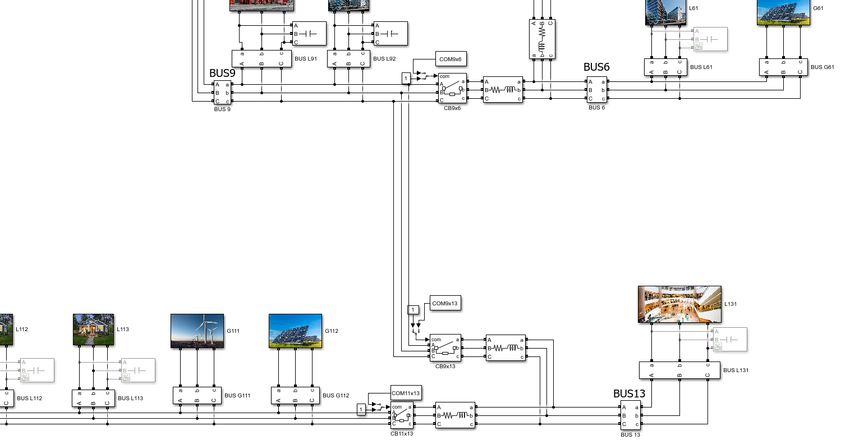
B.1 Figure of the entire Simulink model . . . . . . . . . . . . . . . . . . . 76
B.2 Close up figure of the network part 1 . . . . . . . . . . . . . . . . . . . 77
B.3 Close up figure of the network part 2 . . . . . . . . . . . . . . . . . . . 77
B.4 Close up figure of the network part 3 . . . . . . . . . . . . . . . . . . . 77
B.5 Close up figure of the network part 4 . . . . . . . . . . . . . . . . . . . 78
B.6 Close up figure of the network part 5 . . . . . . . . . . . . . . . . . . . 78
B.7 Close up figure of the network part 6 . . . . . . . . . . . . . . . . . . . 79
B.8 Close up figure of the network part 7 . . . . . . . . . . . . . . . . . . . 79
C.1 Charging station example with random power inputs . . . . . . . . . . 81List of Tables
3.1 MATLAB vs GNU Octave vs Scilab Comparison . . . . . . . . . . . . 19
3.2 Simulation variables, their default value and explanation . . . . . . . . 40
4.1 Poor performance simulation periods . . . . . . . . . . . . . . . . . . . 45
viiGlossary
DER Distributed Energy Resources. 4
DLMP Distributed Locational Marginal Pricing. 2
DN Distribution Network. 14, 31
DPF Displacement Power Factor. 14, 15
GECAD Research Group on Intelligent Engineering and Computing for Ad-
vanced Innovation and Development. 3
HVDN High Voltage Distribution Network. 8, 30
ICT Information and Communication Technologies. 5
LVDN Low Voltage Distribution Network. 32
MVDN Medium Voltage Distribution Network. i, ii, 1, 2, 4, 5, 7–9, 13, 16, 17,
19, 20, 22, 24–28, 30, 31, 33, 35, 42, 43, 52, 57, 58, 63–65
ODE Ordinary Differential Equation. v, 20–25, 40, 42
PMU Phasor Measurement Units. 5
PV Photo Voltaics. 1
RES Renewable Energy Sources. 5, 6, 16
SC Smart City. 2, 4
SG Smart Grid. 1, 2, 4, 6, 22, 27, 28, 35
SLG Switching, Load and Generation. 40
ixAcknowledgements
I would like to start off by thanking KULeuven and ISEP for giving me the
opportunity to go on an international student exchange. I want to thank Bruno
Canizes, João Soares and Simon Ravyts for guiding me through the process of
writing a master thesis. Besides learning about simulations and medium voltage
distribution networks in a smart grid context, I learned a lot about myself as a
person here. This experience was unforgettable and I will look back on my time
in Porto with a big smile on my face.
Verder zou ik ook graag mijn ouders bedanken, die altijd in mij geloofden.
Zij hebben mij de kans gegeven om te doen wat ik het liefste doe, op school vlak
en daarbuiten, en hebben daarbij mede bijgedragen tot de persoon die ik nu ben.
Mijn broer Nicolas en zus Sarah zou ik ook graag willen noemen. Ik ben heel
trots op hen en ook zij zijn elk op hun eigen manier een grote steun geweest. Als
we het dan over Porto hebben, zou ik graag La Colove en in het bijzonder Ismael
Zighed willen bedanken. De ontelbare uren die ik in goed gezelschap daar heb
doorgebracht, werkend aan deze thesis, zullen mij zeker bijblijven. Verder gaat
mijn hart ook uit naar The Fellowship, stuk voor stuk topkerels die bij hebben
gedragen tot een onvergetelijke ervaring hier. Alessandro, Philipp, Kevin, Marco
en Ismael, ik zie jullie snel weer. Op deze manier zou ik ook de andere mensen
willen bedanken die mijn tijd hier onvergetelijk hebben gemaakt: Breyner House,
en in het bijzonder Lotta en Sarah, Joy house en Villa Moreira, mijn huisgenoten.
Jullie weten wie jullie zijn. Ik kan mijn dankbaarheid naar iedereen genoemd
hierboven maar moeilijk in woorden uitdrukken.
Thank you for everything, see you soon!
xiChapter 1
Introduction
In the following chapter a brief explanation will be given about the goals and
objectives of this thesis, the main problem this work is trying to contribute to
solving and the motivation for chipping in to the solution. Requirements for
the understanding and recreation of the thesis and the overall structure of the
dissertation can also be found in this chapter.
1.1 Problem
In a rapidly changing globalised world where combustion engines and fossil fuels
are slowly phased out [1] in favor of more ecological and durable energy solutions,
the current Medium Voltage Distribution Networks (MVDN) will have to adapt
accordingly. As one might imagine, if everyone comes home from work in the
evening and plugs in their electric vehicle (EV) at the same time, there will
be a surge in the electric energy demand. This impact on the grid can not be
underestimated [2]. Combining this with the fact that the overall penetration
of photo-voltaic (PV) and wind energy has been increasing [3], the distribution
network should also be able to handle the rapidly changing power flow in the
grid due to the fluctuating character of renewables [4], for networks with a radial
topology, this is however not obvious [5]. This implies quite a few challenges along
the way as the current MVDN is not ready yet to handle this more complicated
approach to energy distribution. Making the necessary changes to adapt the
network to its new workings and exploiting the MVDN as a smart grid (SG)
looks like the way forward as it offers a lot of advantages over the more traditional
approach of having central production units supply the downstream consumers
with electrical energy [6].
12 CHAPTER 1. INTRODUCTION 1.2 Motivation The evolution of people moving to big cities in favor of the countryside in recent years has a big impact on the energy needs and quality of the air in these cities. Cars and fossil fuel energy plants contribute for a big part to the air pollution present. EV’s and renewable energy sources make for an excellent solution to this problem. It is in everyone’s interest to make the city life appealing and healthy and uphold and improve the overall quality of life. With this work, I hope to make a small contribution to a healthier and more sustainable way of living in Smart Cities (SC). 1.3 Objectives The goal of the following work is to give a deeper understanding in the solid state behaviour of a SG using a modeling software, in this case MATLAB simulink. Similar works have been made in the past, but then with different software pack- ages [7] [8]. This inexpensive method can give insight in the behaviour of the net- work in a lot of configurations without the need to build and test a real MVDN. Moreover, the model can give us a good idea on how to optimally implement certain parts of a similar network in an actual city. The first part to achieving this lies in the development of and/or use of models for each of the different components of the SG. Famous in the computer science and information theory is the saying: ”Garbage in, Garbage out”. The same holds true for models. If a model of a component does not behave closely to the real object, any input in this model will result in an output that doesn’t come close to the behaviour of the object that it was modelled after. This implies that we have to take extra care when developing/picking a model for each of the components. Simulink includes a lot of toolboxes which contain many tried and true models for a lot of the components used in the MVDN. Once the models for the different components have been decided on, the model is assembled as a whole and collected data from an optimal distribution grid op- eration algorithm using DLMP-based pricing [9] from 19/03/2017 will be fed to the MVDN. The output data from the model will then give us a good idea on how the SG behaves at different times of the day. Along the way, a few challenges had to be overcome to extract useful information from the MVDN simulation. One element in particular, responsible for con- necting and disconnecting certain busses from each other, proved to be quite a challenge to implement. The complications this component created, along with the possible causes and the solutions proposed will be presented in this work. Afterwards, the results of the simulation will be shown and discussed. As a final objective, a conclusion will be drawn from the obtained results and suggestions on how to expand on this work will be given. It is important to remark that
1.3. OBJECTIVES                                                               3

the definition of the objectives of this work has benefited from the interaction
with national and international RD projects coordinated by or having the par-
ticipation of the Research Group on Intelligent Engineering and Computing for
Advanced Innovation and Development (GECAD), where this thesis has been
developed. The breakthrough nature of these projects has enabled this thesis
to consider innovative perspectives that have helped to enrich this work. The
considered project is: CENERGETIC – Coordinated energy resource manage-
ment under uncertainty considering electric vehicles and demand flexibility in
distribution networks, reference PTDC/EEI-EEE/29893/2017.
4                                                 CHAPTER 1. INTRODUCTION

1.4    Requirements
As the main goal of this thesis is to obtain usable results regarding the operation
and reconfiguration in a smart grid context in simulink, a MATLAB/simulink
license of version 2020b or above is required to run the model and simulations
discussed in the following chapters. Besides this, an understanding of the basic
laws of electricity, electrical components and the different parts of an electrical
energy grid are required to thoroughly understand the following work.

1.5    Structure of the Thesis
The following thesis will contain 5 chapters. The first one being the introduction,
where the motivation for this work, the objectives that have been set and the
requirement for this dissertation were listed.
Following this chapter, we get to the 2nd chapter, where information about MVDN
in a SG context is listed, compiled down to a summarized and digestible format,
to give the reader more insight into the matter before continuing with the rest of
the work. The discussed works in this chapter should give some deeper insight
on the subject and serve as a reference for the work that will be presented in the
following chapters.
The 3rd chapter will start off with the reasons MATLAB Simulink was chosen
as the software environment to run the MVDN simulation on. This is followed
by an explanation on how simulations in Simulink are evaluated by a computer.
The different types of solvers used to solve the inherent differential equations
of the model are compared against each other until a suitable solver is decided
on. The development and implementation of every model used inside simulink
will be discussed after. A deeper look will be taken at every component chosen
and how it will be used to reinforce the model. This will explain how we go
from the BISITE’s (https://bisite.usal.es/en) mock-up SC with 13-bus MVDN
and high penetration of Distributed Energy Resources (DER) to modelling the
entire network inside the Simulink environment.
The 4rd chapter starts off with an explanation of the challenges faced on the
way when coming up with a working MVDN model, the problems encountered
and the possible solutions. The remaining part of this chapter will consist of
the discussion of the results obtained by running the model. This chapter will
contain the network data condensed down into graphs. To finish the structure
of the thesis we will end with a general conclusion about the dissertation and
suggestions on how to expand this work in the future.
Chapter 2

Medium Voltage Distribution
Network in a Smart Grid Context

 Chapter 2 will shortly go over some literature regarding smart MVDNs. A deeper
look will be taken into each of the MVDN components and how they make up a
distribution grid as a whole.
     Before going over MVDNs and the elements out of which they consist, a look
will be taken at the smart part of a smart MVDN. Verbong G et al. published
a paper about smart grid experiments in the Netherlands where they state the
increasing introduction of renewable energy sources and the popularisation of
’s and heat pumps prove to be a challenge for the aging energy distribution
infrastructure [10]. The simple solution suggested is the reinforcement of the
network by replacing the old cables with heavier ones. This might prove to be
only a short term solution as the share of renewables, EV’s etc. in the network
will keep increasing at an unknown pace. The more long term approach is to
upgrade to a more intelligent distribution networks, called smart grids. [11] [12]
[13] These utilise Information and Communication Technologies (ICT) combined
with advanced measuring devices such as Phasor Measurement Units (PMU)
equipped with GPS receivers that allow for synchronisation of data from varying
distances [14]. This way the grid is made more ’intelligent’ as changes to the
network connections can be made on the fly, based on real-time info across the
entire network. Certain network components are even specifically designed and
tailored to be used within a smart grid network [15] [16]. All these combined
makes the network more robust and sustainable as well as improving the overall
efficiency by reducing the network losses [17].
    According to Lund et al [18] there are three phases in the implementation
of renewable energy sources (RES). Most European countries are still in the

                                        5
CHAPTER 2. MEDIUM VOLTAGE DISTRIBUTION NETWORK IN A SMART
6 GRID CONTEXT
introduction phase where there is no or only a small share of renewable energy in
the electrical energy system. SGs will offer a big advantage over traditional grids
when we get to the second phase, The large-scale integration phase, where a large
part of the energy in the system has a renewable character. Due to the higher
penetration of these RES and their dependence on wind, solar radiation etc., the
direction and magnitude of the power flow can change drastically within a very
short time span. This implies that the stability of frequency and voltage will have
to be monitored closely as the network frequency is linked to active power balance
in the grid and the voltage supplied is linked to the imaginary power balance [19].
The third phase is the 100% renewable energy phase where all demand of electric
energy is met by renewable energy generation. This is definitely something for
the far future as there are a few concerns right now regarding 100% renewable
energy. First of all the scale at which renewable energy is used would have to
go up immensely to compensate for the disappearance of traditional and non-
renewable resources. It will take a lot of time and resources and as of now there
is not much economical incentive to make this transition. The second concern is
the irregular character of most renewable energy. Solar and wind for example are
highly dependant on solar irradiation and wind velocity. Factors that lie out of
human control. This implies a challenge to meet the growing demand of electrical
energy at times where RES alone are not producing sufficient power to meet this
demand. The use of energy buffers might provide a solution here.
2.1 Distribution lines
To be able to speak of a distribution network, Electrical energy needs to be
distributed over medium to long distances. The focus in this distribution lies on
keeping the distribution losses as low as possible. Apparent power is transported
through the lines. Take the following equation into account:
∗
S =V ·I (2.1)
Where S stands for apparent power, V for voltage and I for current, with the bar
signifying complex notation and the asterisk standing for complex inverse nota-
tion. Most of the losses in a distribution line have a thermal nature. Since these
losses are linked to the square of the current flowing through the line Pth = R · I 2 ,
we can reduce the losses by transforming the voltage to a higher one before trans-
port (see substations later). By increasing the voltage level, the current lowers
for transport of the same amount of power. These thermal losses will definitely
have to be taken in account when developing a distribution line model. The
second type of distribution losses that impact the efficiency of the lines are para-
sitic capacitance losses. When two conductors with a high difference in potential
electrical energy come close to each other, charges of opposite polarity will arise2.1. DISTRIBUTION LINES 7
in each of the conductors due to the electric field between them. This basically
means they work as a capacitor. This parasitic capacity will draw current to nul-
lify the built up charge in the conductors as described in the following equation:
dv
i=C (2.2)
dt
Where
Q
C= (2.3)
V
As MVDN usually go up to 35kV and can be quite lengthy, the leakage currents
associated with these parasitic capacitances can not always be neglected.
2.1.1 Transmission line theory
To model a transmission line, we should start from the physics equations that
describe the behaviour of the line. In 1876, Oliver Heaviside published the first
work from his Transmission Line Model. This model shows that electromagnetic
waves are reflected along a transmission line where the sent signal and each of
its reflections can be described using the Telegrapher’s equations. These are two
partial differential equations that describe the relationship between voltage and
current along the transmission line, as a function of time t and place z [20].
∂ ∂
v(z, t) = −R · i(z, t) − L · i(z, t) (2.4)
∂z ∂t
∂ ∂
i(z, t) = −G · v(z, t) − C · v(z, t) (2.5)
∂z ∂t
where L, C, R and G are given per unit of distance. Both equations can then be
combined to write an equation that only depends on one variable:
For the voltage:
∂2 ∂2 ∂
2
v(z, t) − LC · 2
v(z, t) = (RC + GL) · v(z, t) + GR · v(z, t) (2.6)
∂z ∂t ∂t
For the current:
∂2 ∂2 ∂
2
i(z, t) − LC · 2
i(z, t) = (RC + GL) · i(z, t) + GR · i(z, t) (2.7)
∂z ∂t ∂t
where LC = µ with µ signifying the absolute magnetic permeability and sig-
nifying the absolute electric permittivity.CHAPTER 2. MEDIUM VOLTAGE DISTRIBUTION NETWORK IN A SMART
8 GRID CONTEXT
It can be noted that in High Voltage Distribution Networks (HVDN), the in-
ductive reactance per km and capacitive reactance per km can be much larger
than the resistance per km and conductance per km, respectively, of the line. In
this case, the resistance can be neglected (R = 0) relative to the inductive reac-
tance and the conductive reactance neglected (G = 0) relative to the capacity.
This means the right side of both equations 2.6 and 2.7.
We are however talking about MVDNs where this is rarely the case as the values
of resistance and conductivity are often too close in magnitude to the reactances.
Figure 2.1: Transmission Theory Model
[21]
In figure 2.1 you can find the Model used to visualize the transmission line
theory. We find the voltage and current at the beginning of the line in function
of the distance z and time t. The end of this piece of transmission line is written
as z + dz, where dz is an arbitrary distance increment. The difference in state
of the voltage and/or current wave at point z and point z + dz is dependant on
the distance increment dz and time increment which means that a longer power
line will result in voltage and current in beginning and end being more out of
sync. It is interesting to think about at which increment dz voltage/current are
most out of sync. Europe, as well as most other regions in the world exploit their
power grids with a fixed frequency of 50Hz. The relation between frequency and
wavelength is connected with the speed of light:
c=f ·λ (2.8)
at a frequency of 50Hz and the speed of light being 300,000 kms , we find that the
wavelength for a 50Hz electrical signal is 6000km. At half the wavelength and at
a certain time t, the difference in position of the voltage wave at the beginning
of the line and at the end will be exactly 2 times the amplitude.
2.2 Substations
As discussed in the section about distribution lines, it became apparent that elec-
trical substations play a very important role in the workings of the electrical grid.
To go from one distribution network to another, it is often necessary to go from2.2. SUBSTATIONS 9
one voltage level to another or shift the phase angle θ to ensure a proper con-
nection between the two networks. When we talk about high power applications,
this transformation of voltage level or shift in phase angle is almost always done
with a transformer. The MVDN that is discussed in this work has a line to line
voltage of 35kV. Substations will be needed to transform the high voltage feeding
the MVDN down to 35kV and to transform the 35kV medium voltage down to a
usable voltage on the low voltage distribution grid.
2.2.1 Transformer construction
Transformers have a primary and secondary coil, both with a number of turns
N1 and N2 [22]. Each coil is wrapped around a side of an iron core. If a voltage
is applied over the first coil, a voltage over the second coil will be induced. This
secondary voltage can be higher or lower, depending on the configuration of the
transformer.
Figure 2.2: Transformer
[23]
The physical principle on which the workings of the transformer rely is Fara-
day’s law:
dφ
e=− (2.9)
dt
If an alternating voltage is applied to the first coil, Faraday’s law tells us that a
magnetic flux is being imposed in the core. This flux, that lags 90° behind on
the voltage, will then travel trough the material of the core until it reaches the
second winding along its path. Here the flux will induce a voltage in the windings
of the second coil. The ratio of voltage on the first coil to voltage on the second
coil is determined by the number of turns on each of the coils according to theCHAPTER 2. MEDIUM VOLTAGE DISTRIBUTION NETWORK IN A SMART
10 GRID CONTEXT
following equation:
e1 e2
= (2.10)
N1 N2
This relation is however only true for an ideal transformer. An ideal transformer
has what we call a ”perfect coupling” between the primary and secondary coil.
This implies that there is no flux leakage from the iron core and all the magnetic
energy induced in the core by the primary coil is converted back to electric energy
in the secondary coil, this basically mean the reluctance of the magnetic core is
equal to 0. The second characteristic of an ideal transformer is that there are no
core- and copper losses present.
2.2.2 No-load losses
The first type of transformer losses, called the no-load losses, are associated with
the core of the transformer. It is a misconception that these losses only occur
when the transformer is not connected to a load. The name just implies that the
losses always happen, no matter the power drawn from the secondary side of the
transformer. Core losses occur when an alternating flux passes through the iron
core of the transformer. They are twofold in nature. On one hand there is the
hysteresis losses[22] [24], they are caused by the residual magnetism in the core
each time the polarity of the flux changes. It takes work to undo this residual
magnetism, which expresses itself in generation of heat. The hysteresis losses
have a thermal nature and can proportionally be expressed as active power lost,
by the empirical law of Steinmetz:
PL,hys = f · (B̂)1,6 (2.11)
It has to be noted that the losses are expressed in [ W kg ] where B̂ stands for the
peak magnetic field.
On the other hand there are the losses due to Eddy currents in the core. Because
of the Joule effect, these currents will cause the core to heat up and contribute to
the overall core losses. The Eddy current losses are proportional to the following
identity:
(f · d · B̂)2
PL,eddy = (2.12)
ρF e
Where d stands for the thickness of the laminations of the core, and ρF e indicates
the resistivity of the core material.
The hysteresis and Eddy current losses together make up the total core losses. If
we take the mass of the core into account:
PL,core = mcore · PL,hys + mcore · PL,eddy (2.13)2.2. SUBSTATIONS 11
Hysteresis losses can be reduced by constructing the core out of an easily mag-
netisable (and de-magnetisable) material, this way the area under the hysteresis
loop, which is proportional to the work required to remove residual magnetism, is
smallest. Electrical steel is often used because of its favourable magnetic proper-
ties. The losses due to Eddy currents can also be heavily reduced by constructing
the magnetic core out of thin (0,3-0,5mm) metal sheets, made out a material with
a high resistivity, that are also electrically isolated from one another. Paper or
a varnish is often used for this purpose. The characteristic buzzing sound that
transformers make is also attributed to the core losses. This is caused by mag-
netostriction, the phenomenon whereby magnetic materials change shape while
being magnetised making the laminations vibrate against each other, producing
the characteristic sound.
2.2.3 Load losses
The second type of losses that occur in a transformer is when a load is connected
to it. These are called the load losses. These are caused by the equivalent
impedance Ze of the transformer. This impedance can be split up in an equivalent
resistance Re and an equivalent reactance Xe . The losses caused by the resistance
are called the copper losses and can be defined as follows:
Pcl = Re · I1 2 (2.14)
The equivalent reactance can then be easily found:
q
Xe = Ze 2 − Re 2 (2.15)
In analog fashion to equation 2.14, the losses due to the equivalent reactance and
impedance as a whole can be found.
2.2.4 Equivalent circuits
Besides the ability to transform voltages up or down, a transformer possesses
another very useful property. The primary and secondary side are in complete
galvanic isolation to each other. This makes it so they can isolate an entire
network from ground. They are commonly used as safety transformers for this
reason as they lower the risk of electrocution significantly due to the leak reac-
tance limiting the fault current.
This same property makes it hard to make calculations with transformer in their
galvanic isolation form. Figure 2.3 shows an equivalent circuit of a single-phase
transformer. Here you can recognise the windings on primary and secondary side
with R0 , R1 and R2 making up the resistances that cause the core losses, copper
losses on primary side and copper losses on secondary side respectively. X0 sym-
bolises the reactance where the magnetisation current Im passes through. ThisCHAPTER 2. MEDIUM VOLTAGE DISTRIBUTION NETWORK IN A SMART
12 GRID CONTEXT
current is responsible for maintaining the flow of magnetic flux in the transform-
ers core. The losses associated with this current are also counted towards the
no-load losses as they remain constant regardless of the load of the transformer.
X1 and X2 signify the equivalent reactances of the transformer related to the
load-losses.
Figure 2.3: Equivalent circuit of a transformer
[25]
To circumvent the problem of a transformer model in this form being hard
to work with, the equivalent T-circuit model was invented. The idea is here that
in this model, the galvanic isolation is taken away and all the voltages, currents
and impedances are referred to one side, generally the primary side.
Since the galvanic coupling is gone now, the model parameters are now dictated by
the transformation ratio k. The relations between parameters when transferred
from secondary to primary is as follows: For the voltage:
E1 = k · E20 (2.16)
For the current
I20
I1 = (2.17)
k
Combining both to find the impedance. Resistance and reactance can be found
in a similar way.
E1 k · E20
Z1 = = = k 2 · Z20 (2.18)
I1 I20
k2.3. SWITCHES 13
Figure 2.4: Equivalent T-circuit of a transformer referred to primary
[25]
2.3 Switches
The next vital component in a MVDN are the power switches. To make a func-
tioning smart grid, the different busses should be able to disconnect from one
another fairly easily. To achieve this, a snubber resistance and/or capacitance
can be added in parallel. The goal is to limit transient voltage peaks when a
switch happens. In a MVDN, the load almost always has an inductive nature.
If the current is suddenly cut, a transient voltage peak will occur. This tran-
sient voltage is even capable of re-igniting the arc caused by opening the switch
[21]. The magnitude of this voltage is dependant on the rate at which the cur-
rent changes with respect to time and the inductance of the load that is being
switched:
di
Vtr = L (2.19)
dt
The resistance (in combination with a capacitor) will dampen this transient by
providing a path for the current to flow when the switch opens, lowering the rate
of current change and reducing the peak voltage over the load. This is beneficial
as arcs are undesirable and make it harder to separate the two sides from each
other. The increased voltage over the load can also damage certain network
elements.CHAPTER 2. MEDIUM VOLTAGE DISTRIBUTION NETWORK IN A SMART
14 GRID CONTEXT
Figure 2.5: Resistive snubber
[21]
2.4 Capacitor banks
A big reason for the use of distribution lines over high voltages to distribute
electrical energy is efficiency. Great effort is put into reducing the loss of energy
and raising the efficiency of an energy system, especially if the energy is in a
noble and highly usable form like electrical energy. Besides distribution losses,
harmonic distortion and the displacement power factor play a big role when it
comes to loss of electrical efficiency. How to reduce distribution losses is discussed
in the section in this chapter about distribution lines. Harmonic distortion also
has to be taken into account since harmonic currents with a frequency above that
of the base frequency do not contribute to the delivery of active power. The total
Harmonic Distortion for the current (T HDI ) can be written as:
Pn
2 I2
T HDI = i=2 i (2.20)
I1
These currents will take up capacity in the lines and possibly congest and in some
cases overload the DN. To reduce the presence of these higher harmonic currents,
low pass filters can used. The working of these low-pass filters depend on the
frequency-sensitive impedance of capacitors.
1
Zc = (2.21)
2π · f · C
As you can see, 2.11 shows that the higher the frequency of the current passing
through a capacitor, the lower the impedance of the capacitor will be. This means
that for high frequency currents, a capacitor between line and ground is basically
a short circuit and these currents will flow to ground, resulting in a lower amount
of harmonic currents, which means the THD will drop and the efficiency will
go up. The third factor that can severely impact the efficiency of an electrical
system is the displacement power factor (DPF).
P
DP F = (2.22)
V · I12.4. CAPACITOR BANKS 15
where If 1 stands for the base frequency current.
As the formula suggests, the DPF (commonly called the cosφ) indicates how
much the current lags/leads the voltage and in turn causes a portion of the
apparent power to be reactive. This will once again lower the efficiency of the
electrical system as the reactive currents will congest and possible overload the
network. Most of the electrical loads fed by a distribution network have either
a resistive or inductive nature. This means in most cases the current will lag
behind the voltage and the reactive power will be positive. To balance out this
positive reactive power, we use what is called a ”capacitor bank”. As the name
suggests, these are devices made up out of capacitors. For three-phase grids,
three capacitors are connected in Y- or ∆ - configuration to one another and
connected to the power lines in parallel. The capacitor banks will provide the
negative reactive power necessary to compensate for the positive reactive power
on the grid, drawn by the inductive loads present. In case the reactive power on
the grid is constant, we can easily calculate the necessary capacity for each of
the capacitors to compensate the reactive power present and raise the DPF. We
start with a certain amount of reactive energy Q that needs to be compensated
for. this means the capacitor banks have to provide the reactive power −Q. We
have to go from necessary amount of reactive power to the impedance value and
thus capacity of the capacitors. Each capacitor bank has three capacitors, one
per phase. Each capacitor can consist out of multiple actual individual capacitors
in series or parallel, for simplicity reasons we use an equivalent capacity in the
formula. Now the equivalent capacity value for each capacitor can be calculated.
The only difference between a Y − and ∆-configuration, is the voltage over each
equivalent capacitor. This will have an influence on the necessary capacity as you
can see below.
for a Y-configuration:
√
3 · (VLL / 3)2 2
Q= = VLL · 2π · f · Ceq,Y (2.23)
Xc
for a ∆-configuration:
2
3 · VLL 2
Q= = 3 · VLL · 2π · f · Ceq,∆ (2.24)
Xc
For both equations, the capacity can easily be found:
Q
Ceq,Y = 2 (2.25)
VLL · 2π · f
Q
Ceq,∆ = 2 · 2π · f (2.26)
3 · VLLCHAPTER 2. MEDIUM VOLTAGE DISTRIBUTION NETWORK IN A SMART 16 GRID CONTEXT 2.5 Conclusions In this chapter we took a look at what the literature had to say about smart grids and MVDN in general. We started off with the advantages of making the transition to this kind of network and what this means for future expansion of RES penetration in networks like these. Next a look was taken at the different components out of which a MVDN exists. The components were described and their use in the network explained. We dove deeper into the distribution lines taking care of electrical transport in the MVDN through the transmission line theory and use this model (although in a permitted simplified form) to set a base for the modeling of these same distribution lines. The electrical substations where next. The transformers used in these substations where explained both in working as well as in the types of losses associated with them. For an accurate simulation, these will all be factors that have to be taken into account. Equivalent transformer circuits where taken into consideration to make the modeling easier without much loss of accuracy. Switches and capacitor banks, particularly how to dimension them properly was briefly explained in this chapter.
Chapter 3

Modeling an MVDN Inside
MATLAB Simulink

In this chapter we will first take a closer look at the methodology of the work. Af-
ter, we continue with comparing some of the software environments that enable
the simulation of a MVDN, this will allow us to find the best tool for the job. To
finalise this chapter, we will go into detail on the models of each of the primary
components of the MVDN. These will be combined into a usable MVDN model,
alongside the MATLAB scripts that aid in the flexibility and automation of the
collection of data from the network.

3.1    Methodology

To simulate and analyse the operation and reconfiguration of a MVDN, first it is
primordial to construct a high-quality model of the network. For every component
inside this network, a model is constructed. Using these individual models and
the topology of the network that has to be modeled, an entire network model
can be constructed. The data on switches, loads and generation in the network
for every period is fed to the model, which will then produce the network results
in the form of currents, voltages and powers for this period. The periodical
data is then combined into a format spanning the entire simulation time. This
concatenated data can then be used to analyse the operation and performance of
the network.

                                        17
18 CHAPTER 3. MODELING AN INSIDE MATLAB SIMULINK
Figure 3.1: Methodology3.2. SOFTWARE ENVIRONMENT 19
3.2 Software environment
In the following section, a quick overview of the most widely used numeric com-
puting environments are displayed in table 3.1. All the software packets are
usable on all the main operating systems. The most important thing that will
have to be taken into account when it comes to an operation and reconfiguration
analysis of a MVDN is the modeling environment of the software. MATLAB,
GNU Octave and Scilab all have their respective modeling environments.
The main advantage of MATLAB over the other two competitors is the exten-
sive library of models provided. The wheel doesn’t need to be reinvented so the
libraries will be used extensively to model the BISITE Smart City. The biggest
downside to MATLAB seems to be the high cost compared to the other two free
software packages. An annual license will set you back $800. You can also opt
for a perpetual license, this one goes for $ 2000. It is worth noticing that GNU
Octave was built with MATLAB users in mind. They are very similar in usage
and functions. Solely because of the size of the available models and the support
associated with MATLAB simulink, this software package will be used for the
modeling of the MVDN.
Table 3.1: MATLAB vs GNU Octave vs Scilab Comparison1
Factors MATLAB GNU octave Scilab
Open source No Yes Yes
Libraries/toolboxes Lots Limited Limited
Platform All All All
Modeling package Simulink built in Xcos
Forums, Help, Manuals All Manual, Forums Manual
Cost High Free Free
1
https://www.mathworks.com/products/simulink.html
https://www.gnu.org/software/octave/index
https://www.scilab.org/software/xcos20 CHAPTER 3. MODELING AN INSIDE MATLAB SIMULINK
3.3 Simulation in general
Translating a MVDN into a usable computer model is a very interesting challenge.
On one hand the goal is to come up with a Simulink model that behaves as close
to the real network is possible. Only if the behaviour is adequately similar, useful
data can be gathered from the network data and valuable conclusions can be
drawn from the analysis this data [26]. Computing power and time are finite and
compromises will have to made along the way to ensure that the simulation can
produce results in a timely manner, as the time span over which you want the
behaviour of an MVDN to be known can be days, weeks or even years.
The model developed for this dissertation was most commonly used to simu-
late the MVDN behaviour based on 15 minute intervals of data during a full day
(24h). It is however capable of simulations with different time intervals at which
the data is presented to the model and a different duration of the total time over
which the behaviour of the MVDN is wished to be known.
3.3.1 Simulation Settings
To achieve accurate results from a simulation, not only modeling each of the com-
ponents as close to real behaviour is important, but also the simulation settings
play a huge part. The model can be perfect and still give sub-optimal results
due to the simulation settings not being very compatible with the to be simu-
lated system. This is why we will dive a little deeper into what makes up these
simulation settings.
3.3.2 Solver
To simulate a dynamic system, the different states of the system are calculated
at consecutive time intervals over a determined total time span. If all the states
of the system are successfully calculated, the system is solved. A solver, meaning
the algorithm that ’solves’ the simulation, or more precisely calculates the states
of the simulation whenever necessary, is actually solving an ordinary differential
equation (ODE) [27] that corresponds to the model. In the case of Simulink these
ODE’s contain one or more derivatives of a dependent variable, in this case y,
with respect to the independent time variable t. The highest order derivative
that appears in the equation is called the order of the ODE. An example of a
second order ODE can be:
d2 y dy
= 2 − 6y (3.1)
dt2 dt
starting from an initial condition y0 at time t0 the ODE can then be solved itera-
tively by applying a particular algorithm to the initial condition and after that the3.3. SIMULATION IN GENERAL 21
results of the previous step, over a total time of tn . This goes on until the current
time tx equals tn . The solver will then return an array with the timestamps of ev-
ery iteration t = [t0 , t1 , t2 , ..., tn ] and their respective results y = [y0 , y1 , y2 , ..., yn ].
The solvers in MATLAB are only able to solve first order ODE’s, these can
be in different forms:
dy
• ODE’s in explicit form = f (y, t)
dt
dy
• ODE’s in linear implicit form M (t, y) = f (t, y) with M (t, y) being a non-
dt
singular mass matrix. This matrix can be state- or time-dependent, as well
as a constant matrix. Encoded in the matrix are the linear combinations
of the first derivative of y involved in linear explicit ODE’s. they can be
dy
transformed into explicit form = M −1 (t, y)f (t, y)
dt
dy
• ODE’s in fully implicit form f (t, y) = 0. These can not be rewritten in
dt
explicit form. There are however some solvers that are specifically designed
to solve this type of ODE.
Any amount of coupled ODE’s can be solved, as long as there is sufficient com-
puting power and memory.
dy
For n coupled ODE’s, with the notation of being replaced by y 0 :
dt
y10 f1 (t, y1 , y2 , ..., yn )
0
y2 f2 (t, y1 , y2 , ..., yn )
.= ..
.
. .
yn0 f1 (t, y1 , y2 , ..., yn )
Since the solvers can only solve first order ODE’s, substitutions are used to
transform the higher-order equations into a corresponding system of the first
order.
y1 = y
dy
y2 =
dt
..
.
dn−1 y
yn = n−1
dt22 CHAPTER 3. MODELING AN INSIDE MATLAB SIMULINK
Using these substitutions, the higher order ODE is solvable by the algorithms.
There are multiple algorithms provided by the Simulink software to solve a
model. all of them have their advantages and disadvantages [28]. The first choice
one has to make regarding the solver used for the Simulink simulation, is whether
it has to be a fixed-step or variable-step solver. The nature of the simulation
you want to run definitely has to be considered when deciding on a variable- or
fixed-step solver. To understand why, the difference between both will first be
explained. As stated above, when solving a system, the different states of the
system are determined at sequential time intervals. What these consecutive time
intervals look is different in both types of solver.
3.3.2.1 Fixed-step solver:
As the name implies, the time intervals or steps are fixed, meaning the time be-
tween each computation is the same for the whole simulation [29]. As this type
of solver does not have an error control functionality built into it, getting a more
accurate simulation result directly depends on lowering the step size, which will
go at the cost of higher computing times. A fixed-step solver is best used when
the magnitude of time constants in the system to be simulated is about the same
for all the components in the network. If there is a subsystem with a very low
time constant (e.g. electrical) combined with a system that possesses a very high
time constant (e.g. mechanical inertia of a concrete-breaker starting up), the
step size will have to be set really low if an accurate simulation of the low time
constant part is desired, even though this low step size is not necessary for the
accurate solving of the high time constant part. A compromise needs to be made
between accuracy and time necessary to simulate. The extent to which there is
a big range of slow- and fast-changing dynamics is called the stiffness. Certain
ODE’s, especially the implicit ones, are much more fit to solve stiff problems.
As the MVDN to be simulated also has some degree of slow and fast changing
dynamics, here we can also talk about a simulation with a certain stiffness.
The second condition in which a fixed step solver is a good idea is when the
changes in the system throughout the simulation happen more or less at a con-
stant rate. Meaning that there are no long periods in which the variables remain
the same followed by short periods of rapid change, e.g. a SG switching states
of operation every 15 minutes, where during this 15 minute interval, no changes
happen. The reason is rather obvious, as the switching behaviour in the MVDN
model is quite difficult to solve and requires a lower step size. The (almost) solid
state of the 15 minutes after the switch however doesn’t require a small step size.
In a fixed-step simulation, the step size of the solver is decided by the part of the
simulation that requires the lowest step size. This also means that the faster to
solve parts are calculated using the same step size, in the end making the time3.3. SIMULATION IN GENERAL 23 required to solve the entire model unnecessarily long. 3.3.2.2 Variable-step solver In this case, the step size is not constant, meaning the time between each com- putation depends on the state of the model. If the model variables are rapidly changing, the step size will shrink to ensure a correct representation of the model results. For longer periods without notable changes, the step size will increase again without decreasing the accuracy on the results. For dynamic simulations where rapid fluctuations in the results are followed by longer periods without many changes, this type of solver is a clear cut winner. Same as with the fixed-step solvers, there are implicit solvers available for when the problem has a high degree of stiffness. Along with this, multi-step solvers also exist within the variable-step category. These solvers will look at the results of multiple previous steps instead of just the last one. In certain scenarios this can give more accurate solutions. It can be noted that certain components inside simulink only work when paired with a certain solver type. This is another big reason why the variable-step type was chosen over the fixed-step. A few of the model components that will follow in section 3.4 require the use of a variable-step solver and so even if the argument for the variable-step type was not convincing enough, this definitely seals the deal. 3.3.2.3 Continuous vs discrete Both the fixed- and variable-step solvers exist in continuous and discrete variants [30]. As the name suggests, a continuous simulation will describe the state of the simulations and its changes over time in a continuous way, meaning that the time variables according to which the simulation changes are not discrete. A continu- ous function, most of the time an ODE, is found that can describe the status of the system at any moment. More often then not, especially in complex systems, an analytic approach to finding the matching differential equation for the system is not possible. Here we will have to resort to numerical computational methods that will approximate what would be the analytic function to describe the contin- uous behaviour of the system. If the right ODE algorithm is chosen for the task, the results can be very accurate. A common usage for the continuous simulation type is physical systems as these don’t have discrete states most of the time and have to be modelled in a continuous way. In the case of this dissertation, where we work with voltage, current and power flows a continuous simulation variant was chosen. This continuous type of running simulations stands in stark contrast to the dis- crete type. Only a simulation with discrete events can be solved by this type of solver. This variant is perfect when the model has a sequence of events that are related to time. Every time an event happens within the model, the state of the
24                    CHAPTER 3. MODELING AN INSIDE MATLAB SIMULINK

system is updated at that time. This variant is used often in economical models
related to sales, logistics,.. as units sold, trucks on the road, units in warehouse
etc. have a discrete nature.

                       Figure 3.2: Simulink solver flowchart
                                       [27]

3.3.2.4    Selected solver

In the end there are a few solvers that meet the criteria needed to solve the
simulation.

     • ODE45(Dormand-Prince): This solver is Simulinks jack-of-all-trades vari-
       able solver. There are little simulations that this solver cannot compute.
       Using an explicit Runge-Kutta (4,5) formula (the Dormand-Prince pair) for
       numerical integration. This is a one-step solver, which means it only needs
       the solution of the previous time step. It is however not always the fastest
       or most accurate. In most cases there is a solver that can do a better job
       in less time. This is why we will look further for a more suitable solver.

     • daessc(Simscape Solver): As the name implies, this solver is specifically
       designed to solve Simscape physical systems.It calculates the state of the
       model at the next time step by solving systems of differential-algebraic
       equations resulting from Simscape models. For the MVDN-simulation it
You can also read