Using Commensurabilities and Orbit Structure to Understand Barred Galaxy Evolution
←
→
Page content transcription
If your browser does not render page correctly, please read the page content below
Mon. Not. R. Astron. Soc. 000, 000–000 (0000) Printed 30 April 2021 (MN LATEX style file v2.2)
Using Commensurabilities and Orbit Structure to Understand
Barred Galaxy Evolution
Michael
1
S. Petersen,1,2? Martin D. Weinberg,2 Neal Katz2
Institute for Astronomy, University of Edinburgh, Royal Observatory, Blackford Hill, Edinburgh EH9 3HJ, UK
2 Department of Astronomy, University of Massachusetts at Amherst, 710 N. Pleasant St., Amherst, MA 01003
30 April 2021
arXiv:1902.05081v3 [astro-ph.GA] 29 Apr 2021
ABSTRACT
We interpret simulations of secularly-evolving disc galaxies through orbit morphology. Us-
ing a new algorithm that measures the volume of orbits in real space using a tessellation,
we rapidly isolate commensurate (resonant) orbits. We identify phase-space regions occupied
by different orbital families. Compared to spectral methods, the tessellation algorithm can
identify resonant orbits within a few dynamical periods, crucial for understanding an evolv-
ing galaxy model. The flexible methodology accepts arbitrary potentials, enabling detailed
descriptions of the orbital families. We apply the machinery to four different potential mod-
els, including two barred models, and fully characterise the orbital membership. We identify
key differences in the content of orbit families, emphasising the presence of orbit families
indicative of the bar evolutionary state and the shape of the dark matter halo. We use the char-
acterisation of orbits to investigate the shortcomings of analytic and self-consistent studies,
comparing our findings to the evolutionary epochs in self-consistent barred galaxy simula-
tions. Using insight from our orbit analysis, we present a new observational metric that uses
spatial and kinematic information from integral field spectrometers that may reveal signatures
of commensurabilities and allow for a differentiation between models.
Key words: galaxies: Galaxy: halo—galaxies: haloes—galaxies: kinematics and dynamics—
galaxies: evolution—galaxies: structure
1 INTRODUCTION While typical rosette orbits in an axisymmetric system fill an area
of the disc after many orbital periods, non-axisymmetries in the
Empirically, a typical axisymmetric disc is dominated by orbits that
system may create new families of commensurate (or resonant) or-
appear to be regular rosettes of varying eccentricities determined
bits1 . These commensurate orbits are defined by the equation
by the radial energy. Such regular orbits have constants of motion
and are considered integrable, and can be represented by a com- mΩp = l1 Ωr + l2 Ωφ + l3 Ωz (1)
bination of three fundamental frequencies. As stated by the Jeans
where Ωr,φ,z are the polar coordinate frequencies of a given orbit
theorem (Jeans 1915) for an axisymmetric system, the distribution
and Ωp is some pattern frequency, e.g. the frequency of a bar or
function is a function of isolating integrals of motion. For example,
spiral arms. Commensurate orbits are closed curves and have for-
in a razor-thin disc, these would be energy E and the angular mo-
mally zero volume, in the sense of the configuration-space volume
mentum about the galaxy’s symmetry axis Lz . This principle has
filled by the orbit, when pictured in a frame rotating with the pat-
been used in a number of analytic studies over the past century (see
tern speed Ωp . One may consider the commensurate orbits as the
Binney & Tremaine 2008), including recent advancements (Binney
backbone around which secular evolution occurs – where E or Lz
& McMillan 2016). Additionally, the Jeans equations (Jeans 1922)
can be gained or lost, for example.
have been used to perform assessments of the content of orbital
Even in the case of relatively simple potentials, such as an
families in a model – the orbital structure – of real galaxies under
exponential stellar disc embedded in a spherical dark matter halo,
the assumption that the galaxies can be described by the classical
finding the distribution function, fundamental frequencies, and/or
integrals of motion: E, Lz , and a third integral commonly referred
commensurate orbit families analytically can rapidly become in-
to as I3 (Nagai & Miyamoto 1976; Satoh 1980; Binney et al. 1990;
tractable, especially in the presence of a modest to strong non-
van der Marel et al. 1990).
axisymmetric perturbation. Any known method for producing an-
Unfortunately, the assumption that galaxies are semi-isotropic
alytic potentials is insufficient for characterising the real universe.
rapidly breaks down for realistic galaxies and dynamical models.
1 In addition to commensurabilities that exist in the axisymmetric disc-halo
? michael.petersen@roe.ac.uk system.
© 0000 RAS
2      Petersen, Weinberg, & Katz

Few axisymmetric potentials that resemble real galaxies can be de-                     Within this framework, many previous studies have used fre-
scribed via separable potentials (de Zeeuw & Lynden-Bell 1985).                  quency analysis to characterise the properties of orbits, describing
Further, the inclusion of non-axisymmetric features, such as a bar,              orbits by their frequencies in various independent dimensions. The
can render the potential calculation intractable2 . Simply changing              result is a partitioning of orbits into families that reside on inte-
the halo model from a central cusp to a central core is known to                 ger relations between frequencies, using equation (1). Attempting
alter the families of bar orbits present near the centre of the galaxy           frequency analysis on an ensemble of real orbits is a natural exten-
(Merritt & Valluri 1999). Thus, it is difficult to constrain the orbital         sion, via either spectral methods (Binney & Spergel 1982; Binney
structure of realistic, evolving galaxies. The lack of techniques in             & Spergel 1984) or frequency mapping (Laskar 1993; Valluri et al.
the literature for determining orbital families in evolving potentials           2012, 2016). However, these tools are only useful when the evo-
applicable to realistic galaxies (e.g. non-axisymmetries) motivates              lution of the system is slow, or the evolution is artificially frozen.
finding new methodologies that determine the orbital content of a                Therefore, we develop a new methodology based on a simple and
disc galaxy. We present techniques suitable for studying orbits in               robust tessellation algorithm that permits the unambiguous deter-
evolving potentials in this paper.                                               mination of commensurate orbits on several orbital time scales en-
      Analytic and idealised numerical studies of potentials repre-              abling analysis in evolving simulations. We emphasise that the util-
senting barred galaxies show a basic resonant structure that un-                 ity of this method extends beyond the proof-of-concept presented
derpins the bar represented by the commensurate x1 orbit, which                  here. An advantage to this orbit atlas analysis is its ability to move
arises from the inner Lindblad resonance (ILR, where 2Ωp =                       beyond the standard methods of locating resonances based on fre-
−Ωr +2Ωφ ; Contopoulos & Papayannopoulos 1980; Contopoulos                       quencies. We are able to empirically determine the location of all
& Grosbol 1989; Athanassoula 1992; Skokos et al. 2002). How-                     closed orbits in both physical and conserved-quantity space.
ever, small adjustments to the mass of the model bar can admit new                     In this paper, we apply this simple methodology and char-
commensurate subfamilies of x1 orbits, necessitating a model-by-                 acterise orbital structure, with a particular emphasis on commen-
model (or galaxy-by-galaxy) orbital census. Such subfamilies have                surate orbits, to understand barred galaxy evolution. This work
been extensively documented in the literature Contopoulos & Gros-                presents significant upgrades to one orbit analysis tool previously
bol (1989); we will discuss and show subfamilies below. For sim-                 published (PWK16), as well as an entirely new algorithm. The goal
ulated galaxies, taking the measure of the orbital structure means               of this project is to develop new techniques for comparing non-
being able to (nearly) instantaneously identify the family of a given            axisymmetric orbits between fixed potential simulations and fully
orbit, as the orbit family may change over a handful of dynamical                self-consistent simulations. We discern distinct phases or epochs
times. Bifurcations of prominent orbit families result from alter-               of evolution of a bar in self-consistent simulations. Along the way,
ations to the potential shape, giving rise to families such as the 1/1           we demonstrate that (1) we can efficiently dissect bar orbits into
(sometimes stylised 1:1) orbit, a family which results from the bi-              dynamically relevant populations, (2) commensurate orbit families
furcation of the x1 family (Contopoulos 1983; Papayannopoulos                    can be efficiently found and tracked through time across different
& Petrou 1983; Martinet 1984; Petrou & Papayannopoulos 1986).                    fixed-potential realisations, (3) commensurate orbits provide a use-
For consistency, we refer to this orbit throughout this work as an               ful method to analyse self-consistent simulations, and (4) one may
x1b orbit, denoting that the family is a bifurcation of the standard             infer the evolutionary phase of barred galaxies from this methodol-
x1 orbit.                                                                        ogy.
      Finding commensurabilities in realistic potentials has proven                    The organisation of the paper is as follows. We describe the
particularly difficult in an analytic framework (Binney & Tremaine               models we studied in the course of this work and present new tech-
2008). Even more difficult is identifying the act of ‘trapping’, or              niques in Section 2. Results from different fixed potential models
capture into resonant orbits, which cannot occur in fixed gravita-               are presented in Section 3. We then discuss the implications of the
tional potentials. Recently, techniques to describe orbits observed              findings for interpreting other models in Section 3.3. We discuss
in self-consistent simulations such as those drawn from N -body                  the implications of the results for observational studies in Section 4.
simulations, i.e., those that are allowed to evolve with gravitational           We then use the lessons from our fixed potential analysis to inter-
responses, have been used to find the rate at which particles change             pret the evolution in the self-consistent simulations in Section 5.
orbit families in response to the changing phase-space structure                 We conclude and propose future steps in Section 6.
(Petersen et al. 2016, hereafter PWK16).
      Despite the effort placed into studying both analytic potentials
and self-consistent simulations, a vast gulf of understanding exists
between analytic and self-consistent potentials. Linear or weakly
non-linear galaxy dynamics can only be extended so far: at some
point, the distortions become so strong that it is insufficient to
consider perturbations to the system and one must treat the entire               2   METHODS
system in a self-consistent manner. However, fully self-consistent               We first present the initialisation and execution of self-consistent
simulations are encumbered by the many parameters necessary to                   disc and halo simulations in Section 2.1. An overview of the im-
describe a galaxy, all of which are difficult to control when de-                proved apoapse clustering orbit classifier for closed orbit identifi-
signing self-consistent model galaxies. Designing model galaxies                 cation presented in PWK16 is discussed in Section 2.2. The po-
that match observations of real galaxies, including the Milky Way                tentials we use for detailed study of fixed-potential integration are
(MW), is a challenging process. Fixed-potential orbit analysis is                described Section 2.3 and the determination of the bar position
often used as a bridge between analytic and self-consistent work.                and pattern speed in Sections 2.3.2 and 2.3.3, respectively. In Sec-
                                                                                 tion 2.4, we describe the creation of an representative ensemble of
                                                                                 orbits for each model that we call an orbit atlas, including the ini-
2  For simple analytic bar potential expressions, extensions of analytic stud-   tial condition population (Section 2.4.1), and integration method
ies are able to make some progress (e.g. Binney 2018).                           (Section 2.4.2).

                                                                                                                    © 0000 RAS, MNRAS 000, 000–000
Commensurabilities in Disc Galaxies                              3

        Potential Number      Simulation Name, Time      Potential Name     Scalelength    Disc Mass     Mhalo (< Rd )       rMh =Md       Pattern Speed
                                                                            Rd [Rvir ]      [Mvir ]        [Mvir ]            [Rvir ]      Ωp [rad/Tvir ]

        I                     Cusp Simulation T   =0      Initial Cusp          0.01         0.025            0.0050           0.0167            90
        II                    Cusp Simulation T   =2      Barred Cusp           0.01         0.025            0.0050           0.0172           37.5
        III                   Core Simulation T   =0      Initial Core          0.01         0.025            0.0022           0.0317            70
        IV                    Core Simulation T   =2      Barred Core           0.01         0.025            0.0024           0.0282           55.6

Table 1. Potential models used in the detailed fixed potential study.

                                                                                   lies in the ambiguity of the central density of dark matter halos in
                                                                                   observed galaxies, including the MW (McMillan 2017). The pure
                                                                                   NFW profile extracted from dark matter-only simulations is cuspy.
                                                                                   The first two potentials have rc = 0 and, therefore, we refer to
                                                                                   these as ‘cusp’ potentials (Table 1).
                                                                                         We embed an exponential disc in the ’cusp’ potential halo in
                                                                                   our first ’cusp simulation’. The three-dimensional structure of the
                                                                                   disc is given as an exponential in radius and an isothermal sech2
                                                                                   distribution in the vertical dimension:
                                                                                                   Md
                                                                                   ρd (r, z) =            e−r/Rd sech2 (z/z0 )                               (3)
                                                                                                 8πz0 Rd2
Figure 1. Circular velocity curves as a function of radius, computed for the       where Md = 0.025Mvir is the disc mass, Rd = 0.01Rvir is the
cusp and core simulations at T = 0 and T = 2. The left panel shows the             disc scale length, and z0 = 0.001Rvir is the disc scale height,
two initial disc models (T = 0, the initial conditions of each simulation),        which is constant across the disc. We set rc = 0.02Rvir (= 2Rd )
while the right panel shows the two barred models (T = 2, after moderate
                                                                                   for the second simulation, and we refer to that simulation as the
evolution in each simulation). Both panels are colour coded as shown above
                                                                                   ‘core simulation’. We tailor ρ0 for the cored simulation initial con-
the panels. The solid lines are the circular velocity at each radius computed
from the monopole for the total system. The dashed (dotted) lines are the          dition such that the virial masses are equal to that of the cusp
monopole-calculated circular velocity for the disc (halo) component only.          simulation, i.e. Mvir,cusp = Mvir,core = 1. We again embed a
                                                                                   0.025Mvir initially exponential disc in this halo (Table 1).
                                                                                        Both simulations presented here have Ndisc = 106 and
2.1     Simulations                                                                Nhalo = 107 , the number of particles in the disc and halo compo-
                                                                                   nent, respectively. The disc particles have equal mass. We employ a
We employ two galaxy simulations, loosely inspired by the MW, in
                                                                                   ‘multimass’ scheme for the halo to increase the number of particles
this work. The simulations used here are updated slightly from the
                                                                                   in the vicinity of the disc. The procedure to generate a multimass
simulations presented in PWK16, including a modestly more con-
                                                                                   halo is as follows.
centrated halo and significantly longer time integration. We justify
                                                                                        Let nhalo (r) be the desired number density profile for halo
both changes at the end of this section.
                                                                                   particles and ρhalo (r) be the desired halo mass density. We solve
                                                                                   the Abel integral equation using a generalised Osipkov-Merritt
2.1.1     Initial Conditions                                                       parametrisation as a function of E and L (Binney & Tremaine
                                                                                   2008) to obtain the corresponding number and mass distribu-
Both simulations feature an initially spherically-symmetric                        tion functions fnumber and fmass 3 . We realise a phase-space
Navarro-Frank-White (NFW) dark matter halo radial profile                          point by first selecting random variates in energy E and an-
(Navarro et al. 1997), which we generalise to include a core where                 gular momentum L by the acceptance-rejection technique from
the density ρh (r) becomes constant with radius:                                   the distribution fnumber . Then, the orientation of the orbital
                    ρ0 rs3                                                         plane and the radial phase of the orbit are chosen by uniform
ρh (r) =                                                                  (2)      variates from their respective ranges. This determines position
              (r + rc ) (r + rs )2
                                                                                   and velocity. Finally, we set the mass of the particle, m =
where ρ0 is a normalisation set by the chosen mass, rs = 0.04Rvir                  (Mhalo /Nhalo )fmass (E, L)/fnumber (E, L). We choose a target
is the scale radius, Rvir is the virial radius, and rc is a radius that            number density profile for our simulation particles nhalo ∝ r−α
sets the size of the core. rs is related to the concentration, c, of               with α = 2.5.
a halo by rs = Rvir /c. The halo has c = 25, consistent with a                          The number density of particles in the inner halo, r <
normal distribution of halo concentrations from recent cosmolog-                   0.05Rvir (= 5Rd ), is improved by roughly a factor of 100, mak-
ical simulations (Fitts et al. 2018; Lovell et al. 2018). We include               ing the mass of the average halo particle in the vicinity of the disc
an error function truncation outside   of 2Rvir to give a finite mass,             equal to that of the disc particles. This is equivalent to using 109
ρhalo,trunc (r) = ρhalo (r) 12 − 21 (erf [(r − rtrunc )/wtrunc ]) ,

                                                                                   equal mass halo particles. For the basis-function expansion, this
where rtrunc = 2Rvir and wtrunc = 0.3Rvir .
      The normalisation of the halo is set by the choice of virial
units for the simulation, such that Rvir = Mvir = vvir = Tvir =                    3  In the particular realisations for this paper, we define the anisotropy ra-
1. Scalings for the MW halo mass suggest that Rvir = 300 kpc,                      dius ra = ∞, such that finding the distribution functions reduces to the
Mvir = 1.4×10¹² M , vvir = 140 km s-1 , and Tvir = 2 Gyr. The                      standard Eddington inversion. However, our approach does not require this
motivation behind generalising the NFW profile to include a core                   choice.

© 0000 RAS, MNRAS 000, 000–000
4      Petersen, Weinberg, & Katz

implies a higher signal to noise ratio for halo coefficients that af-      the dynamical mechanisms behind bar evolution in the real uni-
fect the gravitational field in the vicinity of the disc.                  verse.
      The disc velocities are chosen by solving the Jeans’ equations
to second order, with asymmetric drift, in cylindrical coordinates
in the combined disc–halo potential, also as in PWK16. The equa-           2.1.2   N-body Simulation
tions are found in Binney & Tremaine (2008). The radial velocity           To integrate not only the N -body model but full orbits, we require a
dispersion is set by the choice of the Toomre Q parameter such that        description of the potential and force vector at all points in physical
                                                                           space and time. We accomplish this using a bi-orthogonal basis set
            3.36Σ(r)Q                                                      of density-potential pairs. We generate density-potential pairs using
σr2 (r) =                                                           (4)
               κ(r)                                                        the basis function expansion (BFE) algorithm implementation EXP
                                                                           (Weinberg 1999). In the BFE method (Clutton-Brock 1972, 1973;
where Σ(r) is the disc surface density, and the epicyclic frequency,
                                                                           Hernquist & Ostriker 1992), a system of bi-orthogonal potential-
κ, is given by
                                                                           density pairs are calculated and used to approximate the potential
           dΩ2c                                                            and force fields in the system. The functions are calculated by nu-
κ2 (r) = r       + 4Ω2c .                                         (5)
            dr                                                             merically solving the Sturm-Louiville equation for eigenfunctions
where Ωc is the circular orbit azimuthal frequency. Our choice of          of the Laplacian. The full method is described in Petersen et al.
Q = 0.9 is motivated by our desire to form a bar in a short time           (2020) for both spherical and cylindrical bases. The description and
period. While our initial conditions are unlikely to be found in the       study of the eigenfunctions that describe the potential and density
real universe, the rapid formation of a bar provides an opportunity        is the focus of a companion paper (Petersen et al. 2019b, hereafter
to study the evolution of a realistic system that resembles observed       Paper III).
galaxies (see Figure 9).                                                         The BFE for halos are best represented by an expansion in
      The disc velocities in each of the three cylindrical dimensions      spherical harmonics with radial basis functions determined by the
(R, φ, z) are realised using a multivariate Gaussian distribution as       target density profile. For a spherical halo, the lowest order ra-
                                                                           dial basis function for l = m = 0 can be chosen to match
vR = x1 σR                                                                 the initial model. To capture evolution, the halo is described by
vφ = x2 σφ + v̄φ                                                    (6)    (lhalo + 1)2 × nhalo terms, where lhalo is the maximum order of
vz = x3 σz                                                                 spherical harmonics retained and nhalo is the maximum order of
                                                                           radial terms kept per l order. This method will work for triaxial ha-
where x1 , x2 , x3 are three random normally-distributed variables         los as well. For triaxial halos, the target density can be chosen to
and the mean azimuthal velocity v̄φ is defined as                          be a close fitting spherical approximation of the triaxial model. The
                            R      d                                      equilibrium will require non-axisymmetric terms but the series will
v̄φ2 (r) = vcirc
            2                                   2     2
                 (r)+                 ρdisc (R)σR (R) +σR (R)−σφ2 (R)      converge quickly.
                        ρdisc (R) dR
                                                                                 The cylindrical basis representing the disc is expanded into
                                                                (7)
                                                                           mdisc azimuthal harmonics with ndisc radial sub-spaces. Each sub-
where vcirc is the circular velocity derived from the potential and        space has a potential function with corresponding force and density
the other terms on the right-hand side correspond to the asymmetric        functions. The lowest-order disc pair matches the initial equilib-
                     2
drift. We assume σR    = σφ2 for these initial conditions.                 rium profile of the analytic functional form given in equation (3).
      To allow the disc and halo to reach a mutual equilibrium, we         Each of these density and potential basis functions are functions
evolve the particles in a fixed disc potential, but live halo potential,   in cylindrical radius R and vertical height above the disc plane
until T = 2Tvir and then restart the simulation with the evolved           z. Just like the spherical basis, the completeness of the biorthog-
positions and velocities. In practice, this allows (1) the halo to con-    onal expansion for the three-dimensional disc is guaranteed by the
tract along the z axis in the presence of the disc, which is only          properties of the Sturm-Liouville equation. Successive terms probe
accounted for as a spherical monopole in the initial spherical halo        finer spatial structure. We truncate the series to follow structure
potential, and (2) any initial rings resulting from imperfect equilib-     formation over a physically interesting range of scales, which has
rium in the disc to dissipate. These rings result from the closure of      the added benefit of reducing small-scale noise including two body
the Jeans’ equations at second order, as well as a theoretical break-      scattering. We may select different features by excluding functions
down of the Jean’s equations at r < z0 , and are O(10−2 ρdisc,0 )          where structural variations are not of interest. A covariance analy-
at all radii, where ρdisc,0 is the initial disc density. The rings phase   sis of the coefficient evaluation shows that our truncation includes
mix within 20 local crossing times. We do not see any evidence that        all basis terms that contribute significant signal. That is, nearly all
the results of our study are affected by the rings. We have checked        excluded terms in our simulations represent Poisson particle noise
that the disc density distribution remains unchanged.                      only.
      As discussed in PWK16, the maximum contribution to the to-                 The potential at any point in the simulation is represented by
tal circular velocity by the disc, fD ≡ Vcirc,? /Vcirc,tot , for typical   (mdisc + 1) × ndisc coefficients for the corresponding orthogonal
disc galaxies is fD = 0.4 − 0.7, with hfD i = 0.57 (Martins-               functions. The disc basis functions are identical between the cusp
son et al. 2013). Our cusp simulation has fD = 0.65 and our core           and core models. The halo basis functions are necessarily differ-
simulation has fD = 0.75. With the new simulations, we evolve              ent to capture the initial density profile in the lowest-order term.
until T = 4.5Tvir . For a MW-mass galaxy, this is equivalent to 9          We retain azimuthal and radial terms (mdisc =lhalo = mhalo 6 6,
Gyr. We acknowledge that it is unrealistic to expect that a galaxy         ndisc 6 12, nhalo 6 20) chosen for both the disc and halo de-
will evolve in a purely secular fashion for half the age of the uni-       pending upon the simulation goals. We discuss the effect on our
verse, without interactions or mass accretion. However, integrating        results owing to the inclusion or exclusion of higher-order harmon-
the simulations for a substantial time allows for a full range of evo-     ics (m = 3, 4, 5, 6) in detail in Section 3.1.3. The halo has a larger
lutionary states to develop as discussed below, which help to probe        number of radial (n) terms to probe similar scales in the disc vicin-

                                                                                                              © 0000 RAS, MNRAS 000, 000–000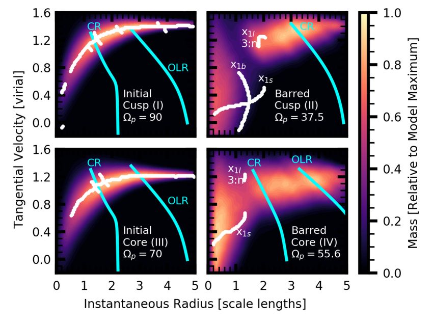
Commensurabilities in Disc Galaxies                            5

                                                                                     of, and support, the potential of the galaxy. The pioneering work
                                                                                     of Contopoulos & Papayannopoulos (1980) presented a census of
                                                                                     bar-supporting orbits, including the principal x1 family. Called the
                                                                                     ‘backbone’ of the bar, x1 orbits exist at various energies set by the
                                                                                     shape of the potential. However, determining family membership
                                                                                     in self-consistent models has been challenging. The concept of the
                                                                                     trapping of orbits into reinforcing structures in the potential is a
                                                                                     dynamically complex, but straightforward, process under idealised
                                                                                     conditions. In the case of perturbation theory, one may compute a
                                                                                     capture criterion or trapping rate (e.g. Contopoulos 1978; Henrard
                                                                                     1982; Binney & Tremaine 2008; Daniel & Wyse 2015), i.e., the
                                                                                     probability that a star on a certain orbit joins a particular resonance
                                                                                     parented by some closed commensurate orbit for which the poten-
Figure 2. Three primary self-consistent bar orbit families classified from           tial may be specified.
the cusp simulation near T = 2. The upper panels are the trajectories,                     In a self-consistent evolving galaxy, the process and probabil-
while the lower panels are the time-integrated densities, or ‘orbit density’         ity of being captured into a resonance–and even the location of the
(i.e. showing where the trajectory moves faster or slower such that an orbit         resonance itself–is difficult to ascertain. Several techniques have
resides at a position for longer). The orbits are organised from largest radial      focused on the use of ‘frozen’ potentials, as follows. First, a model
extent to smallest, with the red bars indicating 0.5Rd in each panel. From
                                                                                     is evolved self-consistently up to some time. Then the potential is
left to right: (a) A standard x1 orbit. (b) A bifurcated x1b orbit. (c) An
                                                                                     frozen and orbits are then integrated in the fixed potential to de-
‘other’ bar orbit, in this case, a nearly 4:2 orbit. All orbits are plotted in the
frame rotating with the bar.                                                         termine the orbital structure. We use a hybrid approach where we
                                                                                     simultaneously analyse frozen potentials and self-consistent sim-
                                                                                     ulations. With input from analytic orbit family descriptions, we
ity. The disc basis is truncated at r = 0.2Rvir or 20 disc scale                     hope to dissect our models using the k-means methodology at ev-
lengths, and |z| = 0.1Rvir outside of which we calculate its contri-                 ery recorded timestep (h = 0.002Tvir ) to determine the constituent
bution using the monopole term only. At large distances d from the                   orbits while the simulation undergoes self-consistent evolution. We
disc, the contribution from terms with m > 0 goes to zero at the                     call the identification of orbit families during self-consistent evolu-
rate d−m faster than monopole. As a result, the spatial truncation                   tion ‘in vivo’ classification. In practice, this means selecting some
of the basis introduces only a maximum 0.3 per cent error in the                     finite time window of the orbit’s evolution, typically 1-2 bar peri-
integration as halo orbits cross this boundary.                                      ods, in which we determine membership in an orbital family. The k-
      EXP allows for an easy calculation of the potential from both                  means classifier is largely insensitive to variations in family mem-
the initial galaxy mass distribution as well as the evolved galaxy                   bership on time scales smaller than the median x1 azimuthal period.
mass distribution. The key limitation of the BFE method lies in the                        The mass that supports the bar feature is a fundamental quan-
loss of flexibility owing to the truncation of the expansion; large                  tity in a barred galaxy model. However, determining the trapped
deviations from the equilibrium disc or halo will not be well rep-                   mass is not an easy task, as we must empirically find parameters for
resented. Although the basis is formally complete, our truncated                     determining trapped orbits in vivo, and both systematic and random
version limits the variations that can be accurately reconstructed.                  errors cause uncertainty. Despite this, our apoapse-clustering tech-
Despite this, basis functions can be a powerful tool to gain physical                nique efficiently locates and identifies orbits that are members of
insight; analogous to traditional Fourier analysis, a BFE identifies                 the bar. The required time resolution is on the order of a handful of
spatial scales and locations responsible for the model evolution.                    turning points per orbit. Other classifiers rely on an instantaneous
                                                                                     spatial or kinematic determination of the disc galaxy structure. The
                                                                                     strength of our apoapse-clustering method is that it depends only
2.2   Computing Trapping                                                             on the positions of the turning points relative to the bar angle. This
We have developed several improvements to the clustering method                      makes the methodology (1) fast and (2) independent of detailed
of PWK16 that enables one to determine the membership in differ-                     simulation processing. The closest analogue to our procedure found
ent orbital subpopulations beyond the bar-supporting orbits during                   in the literature is that of Molloy et al. (2015), who used rotating
the simulations. For example, consider a periodic bar-supporting                     frames to more accurately calculate the epicyclic frequency. How-
x1 orbit. The angle of the apoapses will tightly cluster at 0 and                    ever, their procedure is only robust for orbits that are not changing
180 degrees from the bar major axis. The PWK16 method used                           their family over multiple dynamical times. Our method is robust
a one-dimensional clustering algorithm to identify this bunching                     to orbits that are only trapped for one or two dynamical times.
of apoapse position angles or individual orbits. From their distri-                        We classify three primary types of bar orbit, with prototypical
bution, one can identify various trapped orbit families. No con-                     orbits for each shown in Figure 2:
clusions from PWK16 change as a result of this upgrade; rather,                        (i) x1 orbits, the standard bar-supporting orbit (panel a of Fig-
the improvements provide a more detailed classification. The more                    ure 2).
sophisticated algorithm builds upon the same apoapse-clustering                        (ii) x1b orbits, a subfamily resulting from a bifurcation of the x1
technique, but uses additional diagnostics related to the distribution               family that are often referred to in the literature as 1/1 orbits (panel
of apoapses within the k clusters to determine membership in orbit                   b of Figure 2)4 .
families. The details of the classification procedure are described in
Appendix A. In this section we give a qualitative overview and dis-
cuss the theoretical motivation behind our cluster-based orbit clas-                 4  The so-called 1/1 orbits are a bifurcation of the x1 orbit family owing
sification.                                                                          to a transverse perturbation with the same frequency as the orbital radial
      The orbits that make up a galaxy model are both a reflection                   frequency (hence 1/1, the ratio of the radial frequency of the orbit to that

© 0000 RAS, MNRAS 000, 000–000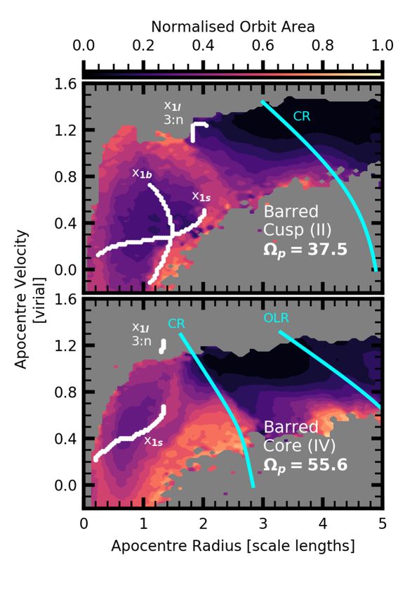
6       Petersen, Weinberg, & Katz

  (iii) ‘Other’ bar-supporting orbits that are coherently aligned
with the bar potential but are not part of the x1 family, generally
demonstrating higher-order behaviour (panel c of Figure 2).
The orbits in Figure 2 are drawn from the cusp simulation as having
been trapped into their respective families at T = 2. Each orbit has
the time series from the cusp simulation T = 1.8 − 2.2 plotted in
the upper row, with the time-averaged orbit density shown in the
bottom row. We refer to the grey scale in the lower row as the ‘orbit
density’, that is, the normalised relative probability of finding an
orbit at a given location in the trajectory. The time-averaged orbit
density is computed using an intentionally-broadened kernel that
more clearly displays the densities. We have plotted only the first
five radial periods in the upper row of panels for clarity in following
the trajectories. In these examples, as in most cases drawn from
self-consistent simulations, the true nature of the orbit is difficult to
determine from the trajectory, but becomes apparent from the time-
integrated location, motivating our inclusion of the time-integrated
location, or ‘orbit density’ in space, throughout this work.

2.3     Fixed Potentials                                                      Figure 3. Frequency versus radius (in disc scale lengths) for the four galaxy
                                                                              fixed potentials. In the barred potentials, we compute the frequency using
We select four example snapshots where we fully decompose and                 the epicyclic approximation computed along the bar major axis. The black
describe the orbit structure, and apply the general results to the evo-       lines plot Ω, which indicates corotation (CR); the lower red lines are Ω −
                                                                               1
lution of barred systems in later sections.                                    2
                                                                                 κ, the inner Lindblad resonance (ILR) and the upper red lines are Ω+ 12 κ,
                                                                              the outer Lindblad resonance (OLR). The dashed grey line is the measured
                                                                              (assumed) pattern speed for the barred (initial) potentials.
2.3.1    Potential Selection
From each of the cusp and core simulations, we compute the fixed              total circular velocity are caused by the halo. The halo models re-
potential at two times, T = 0Tvir and T = 2Tvir , in which we will            main largely unchanged between the Initial and Barred version of
characterise the orbital structure. At each time, we compute the co-          the models, with modest ( 2 components in the bar. See the studies of          modestly from the m = n = 2 harmonic. However, the larger-
Contopoulos (1983), Papayannopoulos & Petrou (1983), Martinet (1984),         scale n = 1 term also contains some spiral-arm power, hence our
Sparke & Sellwood (1987).                                                     choice to use m = 2, n = 2.

                                                                                                                    © 0000 RAS, MNRAS 000, 000–000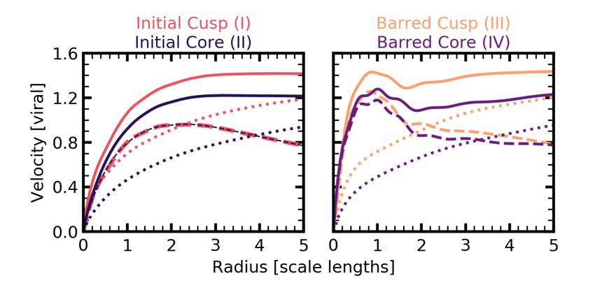
Commensurabilities in Disc Galaxies                         7

2.3.3    Figure rotation                                                     the angular momentum of a circular orbit at the same radius, i.e.
                                                                             X ≡ Lz,orbit /Lz,circular to create a roughly rectangular grid that
The dynamics and orbital structure are driven by the pattern speed
                                                                             extended from radial to circular obits. However, for an analysis
of the bar, Ωp . The rotation of the model introduces the Coriolis
                                                                             of a strongly non-axisymmetric system, the use of axisymmetric
and centrifugal forces in the bar frame, which depend on Ωp . For
                                                                             orbit quantities (e.g. Lz,circular ) is inappropriate. For this work,
the barred potential models, we determine Ωp by calculating finite
                                                                             we choose a more observationally-motivated set of dimensions:
differences in the rate of change of the coefficient phase in a finite
                                                                             turning point radius (Rturn ) and turning point tangential velocity
window of the time series of coefficients from the self-consistent
                                                                             (Vturn ), where Ṙ = 0. One may still find a dominant closed-orbit
simulation. We calculate the uncertainty in Ωp to be 5 per cent. For-
                                                                             family that is analogous to the circular orbit in an axisymmetric
tunately, we find that variations of 5 per cent to the pattern speed
                                                                             case, and we define Vclosed at any given radius, which we use as a
make little difference to the resultant orbital structure. For the initial
                                                                             signpost for interpreting the atlas of orbits.
potentials, Potentials I and III, we test two pattern speeds: Ωp = 0,
                                                                                   In a real system, orbits will typically be observed close to
which reveals the unperturbed structure of the disc and halo sys-
                                                                             apocentre. Therefore, we will generally discuss Rapo and Vapo for
tem, and an estimated Ωp from the self-consistent simulation. We
                                                                             orbits, and restrict our discussion to those orbits where Vturn =
estimate Ωp using the coefficient phases as above for the earliest
                                                                             Vapo and Rturn = Rapo along the bar major axis. We construct the
time when Ωp can be measured: T ≈ 0.2. For the initial cusp we
                                                                             atlas by integrating orbits in a potential obtained from the BFE at
use Ωp = 90 and for the initial core we use Ωp = 70. We apply
                                                                             a particular time. We apply the bar pattern speed, as described in
these pattern speeds to the T = 0 potential models below. As we
                                                                             section 2.3.3, to m > 0 subspaces. We release orbits with turning
shall see, the introduction of figure rotation, and thus Coriolis and
                                                                             points along the major axis of the bar potential. We have inves-
centrifugal forces, reveals that orbital structure varies with Ωp .
                                                                             tigated other release angles, but find that the bar axis is the most
      In Figure 3, we show the primary resonance locations from
                                                                             illustrative of the dynamics. In certain cases, it is necessary to use
epicyclic theory using the gravitational potential along the bar ma-
                                                                             off-axis release angles to find orbits that are known to be relevant
jor axis for the measured bar pattern speed. The left panels plot
                                                                             (described below), but we do not perform an exhaustive search of
the initial potentials (Potentials I and III) and we see that lowering
                                                                             parameter space. We reserve a detailed study of the off-axis release
the assumed pattern speed moves the calculated corotation radius
                                                                             angles for future work. While our orbit atlas does not fully sam-
outward. We also observe that the ILR does not exist at all in the
                                                                             ple phase space, this ‘pseudo-phase-space’ gives a intuitive under-
initial core model for all realistic values of Ωp . The outer Lindblad
                                                                             standing of the system, and can be directly applied to observations.
resonance (OLR) exists for all values of Ωp . However, in the barred
                                                                                   For this study, we also restrict orbits to the disc midplane for
cusp, the radius of the OLR occurs at such large radii (and thus low
                                                                             simplicity. The inclusion of non-planar motion would be straight-
stellar density) so that it would have little influence on the struc-
                                                                             forward, although the phase-space is complex to explore. We will
ture of the disc. In the right panels, we plot the barred potentials
                                                                             investigate vertical commensurabilities in future work. We choose
(Potentials II and IV) and compute the frequency by using Φ(r)
                                                                             to uniformly sample the Rturn − Vturn plane. Our atlas makes no
along the major axis of the bar using the epicyclic approximation.
                                                                             attempt to follow the phase-space distribution of our galactic mod-
As we shall see below, the potential along the major axis of the
                                                                             els. So in principle, the same orbit could be generated both at Rperi
bar better estimates the frequencies in a self-consistent simulation
                                                                             and at Rapo . However, this ambiguity does not affect our goal of de-
than any other strategy. Calculating frequencies using Φ(r) along
                                                                             scribing the structure spanned by the allowed orbit families. Rather,
the minor axis of the bar results in a shallower potential profile,
                                                                             it allows us to compare the initial orbits with orbits in strongly non-
and thus the resonances move inward. In both the right panels, we
                                                                             axisymmetric systems. Similarly, the atlas includes phase space
assume the calculated pattern speed to estimate the location of the
                                                                             that may not be occupied in the simulations (e.g. nearly radial or-
key resonances. The presence of the bar, despite the increased con-
                                                                             bits at large galactic radii). We choose Rturn ∈ (0.2Rd , 5Rd ) and
centration of mass (obvious in the changed circular velocity curve
                                                                             Vturn ∈ (−0.2Vvir , 1.6Vvir ). Our limit of Rturn > 0.2Rd restricts
at r < 2Rd , cf. Figure 1), results in the location of the key res-
                                                                             our analysis to regular orbits. We will return to the question of cen-
onances occurring at larger radii than in their initial counterparts.
                                                                             tral orbits in future work. Our limit of Rturn < 5Rd restricts our
The bar perturbation and the mass rearrangement resulting from
                                                                             analysis to the region that contains all of the interesting commen-
secular evolution create an ILR in the barred core potential (Poten-
                                                                             surabilities.
tial IV) where none existed in the initial core case (Potential III), as
                                                                                   We wish to explore the entirety of the relevant phase space and
well as creating a second ILR at a larger radius in the barred cusp
                                                                             from an initial study of the simulations we see that retrograde orbits
potential (Potential II).
                                                                             play some role in the dynamics of the disc at small radii. Hence, we
                                                                             truncate Vturn at Vturn = −0.2Vvir to study the relevant retrograde
2.4     Orbit Atlas Construction                                             phase space. Similarly, at large Vturn , some orbits may occasionally
                                                                             be driven to large velocities at a given radius by a non-axisymmetric
We detail the construction of an atlas of orbits for the four fixed          potential, joining new orbit families.
galaxy potentials described above. The atlas consists of a time-
series of orbits for each model with a range of starting points. In
section 2.4.1, we describe the starting points for these orbits. In          2.4.2   Integration
section 2.4.2 we describe both the procedures for orbit integration          In the rest of this section, we describe specific details of our integra-
and the details of our implementation.                                       tion scheme, based on the leapfrog integrator used in EXP. Our inte-
                                                                             grator includes the following features beyond the standard leapfrog
                                                                             integrator: (1) an implementation of adaptive timesteps from EXP,
2.4.1    Orbit starting point selection
                                                                             described in PWK16, with minimum timestep thresholds; (2) com-
In PWK16 we describe phase space using energy and angular                    pletion criteria set by either total integrated time or the number of
momentum. Angular momentum was expressed as a fraction of                    apoapses encountered. We use the minimum timestep in the self-

© 0000 RAS, MNRAS 000, 000–000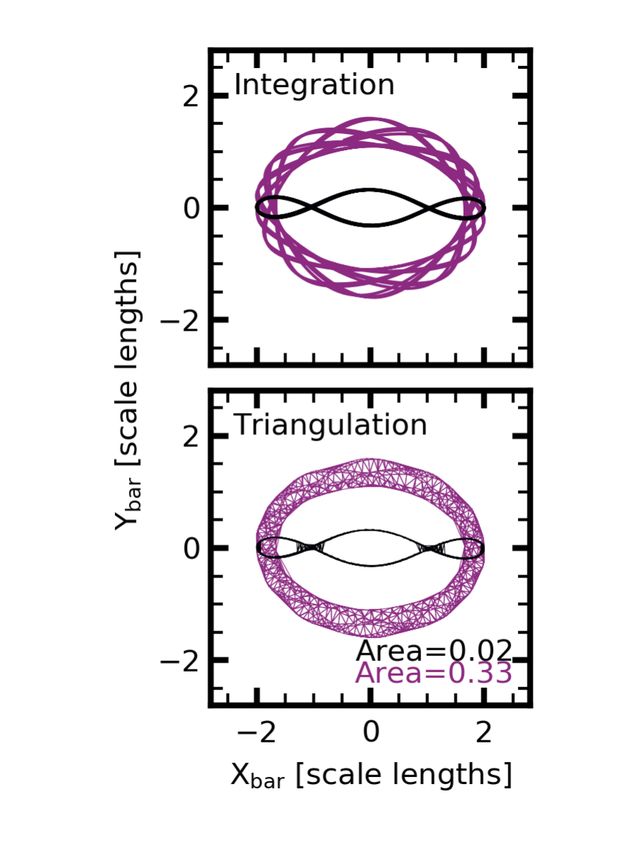
8 Petersen, Weinberg, & Katz
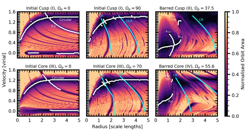
Figure 4. Orbit-area diagrams as a function of radius and tangential velocity, where only orbits with Ṙ = 0 along the bar major axis are shown. We include
two values of Ωp for each of the initial models. The colour map runs from 0 (an orbit which is closed) to 1 (an orbit which completely fills the area of a circle
with radius Rturn ). In each panel, we highlight and label key commensurabilities identified with the tessellation algorithm in white. We plot and label the
locations of corotation and the outer Lindblad resonance, as computed numerically from the monopole where possible, in cyan. The commensurabilities are
discussed in detail in Section 3.1 for the cusp model and Section 3.2 for the core model. The grey region at 0.0 < Rd < 0.2 was not integrated, owing to the
limits of numerical resolution in this study. Some orbits may be shown twice; once at Rapo and once at Rperi , reflecting where they may be observed along
the bar major axis.
consistent simulations, dtvir = 3.2 × 10⁻⁵ Tvir . We truncate the 2.5 Tessellation Algorithm
evolution after 50 radial periods have been completed or a maxi-
mum of ∆T = 0.64Tvir .
We use Delaunay triangulation (DT) to compute the physical vol-
We define each component with a unique set of basis func- ume that an individual orbit occupies, transforming a discrete time-
tions. The orbit integration may use the full potential from the sim- series of (x, y, z) to a volume. For our restriction to the disc plane
ulation or a subset of basis functions for computational efficiency in this study, the two-dimensional DT yields an area. We have
and accuracy. By excluding higher-order terms that do not influ- tested three-dimensional DT, and will make vertical commensu-
0
ence the integration of individual orbits, we can achieve n−n n
or rabilities that are revealed in three dimensions the focus of future
02
1 − ll2 per cent speedups, where n (l) is the total number of radial work.
(azimuthal) halo functions and n0 (l0 ) is the number of retained ra-
dial (azimuthal) halo functions. After inspecting the signal-to-noise We use the DT algorithm with the triangle heuristic described
ratio in the coefficients, we choose not retain higher order halo az- in Appendix B to compute the orbit areas, A, in the Rturn − Vturn
imuthal terms with l > 2, resulting in an 88 per cent speedup of the plane described in Section 2.4.1. We refer to this as the closed-
halo calculation, without any significant differences in the results. orbit map, for its utility in identifying closed orbits. The loci of
We leave our integration flexible in the following ways: (1) A ≈ 0 defines orbit families, which we refer to as valleys. Valleys
the number of azimuthal harmonics in the disc may be specified at may be strong (wide valleys with large regions of A ≈ 0) or weak
run time, which allows for restriction to the monopole contribution (narrow valleys with only a small path satisfying A ≈ 0). The
only and of eliminating odd harmonics; (2) the range of radial basis valleys provide a skeleton of the orbits in a given potential, tracing
functions, which allows for testing the role of low signal-to-noise the commensurate orbits that support the structure of the galaxy
coefficients; and (3) varying the bar pattern speed. We do not apply model. We, therefore, refer to the figures that show the orbit area at
odd-order azimuthal harmonics, which are empirically determined each point in the Rturn − Vturn plane as orbital skeletons.
in the self-consistent simulations to have a different pattern speed
than the even multiplicity azimuthal harmonics. In principle, we The identification of commensurate orbits provides an im-
could use different values of Ωp for individual harmonic orders, e.g. portant theoretical link between a perturbation theory interpre-
Ωp, m=1 and Ωp, m=2 , allowing for an investigation of the dipole’s tation and fully self-consistent simulations (Contopoulos & Pa-
influence separately from that of the quadrupole. We aim to study payannopoulos 1980; Tremaine & Weinberg 1984; Weinberg &
this phenomena in future work. Katz 2007a,b) to find and describe trapped orbits.
© 0000 RAS, MNRAS 000, 000–000Commensurabilities in Disc Galaxies 9
Figure 5. Six example integrations from the Barred Cusp (II) model. In each column, we show the trajectory (upper panel) and time-integrated density (lower
panel). Panels a and b show orbits from the x1b family, where panel a is a ‘symmetric’ x1b orbit (an ‘infinity’ orbit), and panel b is ‘asymmetric’ (a ‘smile’
orbit). Panel c shows a strong x1 orbit. As it is a shorter period x1 than another x1 subfamily at this value of Rapo , we call this an x1s orbit. Panel d shows
a derivative of an x1 -like orbit with higher-order structure and a long period, which is an ‘other’ orbit in our classification. Panel e shows a 3:2 orbit. Panel f
shows a corotation (CR) orbit. In each of the upper panels, the red scale bar is half a disc scale length. All orbits are plotted in the frame rotating with the bar.
3 FIXED POTENTIAL STUDY RESULTS with the non-rotating axisymmetric models to describe the unper-
turbed commensurabilities (Sections 3.1.1 and 3.2.1). We then im-
We apply the tools described above to the potentials described in pose a pattern speed upon the axisymmetric models (Sections 3.1.2
Section 2.3 with the goal of locating and identifying the orbit fam- and 3.2.2), followed by the bar-like non-axisymmetric models in
ilies in each. Closed-orbit maps for the six orbit atlases calculated Sections 3.1.3 and 3.2.3. In Section 3.3, we present the results
from the four potential models are shown in Figure 4. Some or- of applying the tessellation algorithm to orbits extracted from the
bits are shown twice; once at Rapo and once at Rperi , if the orbit self-consistent simulation. We compare the differences between the
is released with Vturn > vclosed (Rturn ). We leave these orbits on fixed potential models and the self-consistent simulations in Sec-
the diagram to facilitate later comparison with self-consistent mod- tion 3.4.
els. The colour map shows the values of the area A, as sampled
by the initial conditions listed above. The colour scheme is uni-
form throughout the paper; colours in Figure 4 may be compared
to the two orbits in Figure B1 for intuition on the colour map. The
white lines in Figure 4 are the identified valleys. We do not plot all
the valleys identified, but rather restrict ourselves to those with dy- 3.1 Cusp Models
namical relevance to bar-driven evolution to avoid confusion. Fur-
ther, for radii beyond the strong influence of the non-axisymmetric 3.1.1 Initial Cusp (I), Ωp = 0
bar force, we use the monopole-calculated frequency to estimate
The zero pattern speed initial cusp potential (Potential I) reveals the
the location of CR and OLR. Near the bar, the non-axisymmetric
commensurate families for a disc embedded in a dark matter halo.
distortions are too large for resonances to be calculated from the
We present the closed-orbit map in the upper left panel of Figure 4.
monopole.
We overlay the orbital skeleton as determined via our tessellation
The valleys track the commensurabilities throughout the bar algorithm.
region, demarcating orbit families. The particular family may be The circular orbit curve (labelled) is the most clearly defined
precisely identified by inspecting orbits from each valley. In many valley. Orbits above this curve will be at pericentre, while orbits be-
cases, the valleys intersect. At these points, we expect to find low this curve will be at apocentre. Crossing the circular orbit val-
weakly chaotic behaviour in a self-consistent simulation. We fo- ley are several m:n commensurabilities, where n is the radial order
cus on regions in phase space around the commensurabilities to and m is the azimuthal order, satisfying equation (1). The 3:2 com-
study the details of secular evolution, such as angular momentum. mensurability (labelled) is the strongest commensurability cross-
Overall, we find similar orbit families to classic analytic studies ing the circular orbit curve. Multiple 3:n families exist in barred
(e.g. Contopoulos & Grosbol 1989; Athanassoula 1992; Sellwood systems, These include the 3:1 family, which has been previously
& Wilkinson 1993). Figure 4 bears some resemblance to the so- studied in the literature (Athanassoula 1992), and is considered a
called ‘characteristic diagram’ found in the analytic literature, al- bifurcation of the x1 family. Some of the 3:n overlap with the x1
though an additional advantage of the closed-orbit map is that the families; this overlap is a channel for bar growth (as described in
steepness of the valley indicates the measure of orbits that resem- Petersen et al. 2019a, hereafter Paper II). The values of m increase
ble the parent; broad low-A valleys imply the existence of many toward smaller radius, such that the next strongest commensurabil-
nearly commensurate orbits. The regions of low area in the closed- ity curve is 5:2, then 7:2, and so on (not labelled). These high-m
orbit map (i.e. A < 0.02) describe the range of librating orbits in and n resonances are not expected to be important for the evolu-
Rturn − Vturn space that resemble the parent orbit (Figure 4). tion of the system. We will confirm this in Section 5. A physically
We first discuss the orbit families in the cusp models before uninteresting radial orbit commensurability valley also appears at
turning to the cored models. For both sets of models, we begin Vapo = 0.
© 0000 RAS, MNRAS 000, 000–00010 Petersen, Weinberg, & Katz
3.1.2 Initial Cusp (Potential I), Ωp = 90 In panel f of Figure 5, we show an example CR orbit in the
barred cusp potential (Potential II), which has a strong CR feature.
The rotating initial cusp, also with the underlying Potential I, has
CR is the lowest-order resonance present in the model, with wide-
structure not present in the non-rotating version of the potential for
ranging dynamical effects for secular evolution discussed exten-
a pattern speed of Ωp = 90, an estimate for the initial formation
sively in the literature (see Sellwood 2014 for a review). CR orbits
pattern speed of the bar (middle left panel of Figure 4). Owing to
are particularly easy to recover using the tessellation algorithm ow-
the axisymmetric nature of the potential, the circular orbit valley is
ing to the tiny area spanned by their trajectory, evident in pane f of
unchanged from the same potential model with Ωp = 0. However,
Figure 5. Owing to the slow precession rates for orbit apoapses near
the radial orbit commensurability seen at Vapo = 0 in the non-
CR in this model, the orbital-skeleton-tracing algorithm described
rotating case is not well defined in the rotating model, occupying a
in Appendix B identifies large regions with A < 0.1 and shallow
negligible region of phase space that is below the resolution of the
slopes of ∂A/∂V and ∂A/∂R, making tracing valleys ambiguous.
closed-orbit map.
This is not a limitation of the algorithm, per se, but rather results
In preparation for using this technique to investigate the dy-
from the low A values in the weakly perturbed, nearly circular outer
namics in a rotating non-axisymmetric potential, we now describe
disc. We, therefore, opt to include only the monopole-derived com-
the commensurate structure in the rotating frame. A rotating model
mensurabilities at radii outside of the bar radius.
admits the familiar low-order resonances, including the inner Lind-
Higher-order azimuthal harmonics of a strongly non-
blad resonance (ILR), corotation (CR), and the outer Lindblad res-
axisymmetric gravitational potential can affect the shape and sta-
onance (OLR). Many higher-order resonances are clearly seen as
bility of orbits in low-order resonance. New families appear owing
low-area (dark) loci. These features correspond to the higher order
to relatively small but important changes in the potential. For ex-
resonances discussed above for the nonrotating model. They are
ample, the exclusion of the m > 2 harmonics from the barred cusp
unlikely to be important in a time-varying potential where the pat-
potential model (II) results in the disappearance of the x1b fam-
tern speed and underlying potential changes faster than the orbital
ily. Inspection of all orbits that are part of the x1b family when
time for a high-order closed orbit.
m 6 6 reveals that the x1b track no longer exists when we restrict
the potential to m 6 2. However, this should not be interpreted as
3.1.3 Barred Cusp (Potential II) evidence that 2 < m 6 6 causes new resonant structure into which
the x1b orbits are trapped, but rather that 2 < m 6 6 distorts the
The non-axisymmetric barred cusp model (Potential II) has orbit potential shape allowed by the quadrupole only into a potential that
families not present in the axisymmetric models. We classify three admits x1b orbits. In Section 5, we will see that x1b orbits are im-
subfamilies of x1 orbits: portant for growing the bar in length and mass. In Figure 6, we
integrate the same orbits as in panels a and b of Figure 5, except
(i) x1b orbits, which may be symmetric or asymmetric about the
that we limit the harmonics included in the potential to m 6 2. The
axis perpendicular to the bar. We show a symmetric ‘infinity’-sign-
orbits are no longer x1b orbits. The infinity morphology x1b orbit
shaped orbit in panel a of Figure 5, and we show an asymmetric
is now a part of the x1 family. The smile morphology x1b orbit has
‘smile’-shaped x1b orbit in panel b (the asymmetric orbits are an
become a ‘rotating boxlet’ orbit6 .
example of an orbit which is more readily identified from an off-
This finding also suggests that m = 2 parametrisations of
axis release)5 .
the MW bar7 , such as those derived from the potential of Dehnen
(ii) x1s orbits, short-period bifurcated standard x1 orbits (with
(2000), (e.g. Antoja et al. 2014; Monari et al. 2016, 2017; Hunt
‘ears’, panel ‘c’ of Figure 5).
et al. 2018), may entirely miss important families of orbits, even if
(iii) x1l orbits, long-period elongated x1 orbits.
the orbits do not appear to exhibit four-fold symmetry. Other recent
We morphologically classified the families identified in Figure 4 models for the MW have suggested the importance of the m = 4
through a visual inspection of the orbit atlas. While many m:n component of the bar for reproducing the observed velocities near
orbits with m > 1 are clearly observed in Figure 4, we choose the Sun (Hunt & Bovy 2018).
to mark only m = 3. Several low-order even n orders comprise In the barred cusp potential (Potential II), CR intersects the
the m = 3 feature, and are indistinguishable in Rturn − Vturn at closed orbit track at Rturn = 3.1Rd . Owing to the relatively slow
the resolution of Figure 4. This is labelled as 3:n in Figure 4. In pattern speed, Ωp = 37.5, CR is at a fairly large radius in this
panel ‘e’ of Figure 5, we plot an example 3:2 orbit. All orbits that potential model; if we assume that the radial terminus of the x1s
are asymmetric across the x-axis in Figure 5 have corresponding
mirror image orbits, where an orbit with one symmetry leads the
bar pattern and an orbit with the other symmetry trails it. With a 6 Some orbits do not show any apparent structure in the inertial frame,
fine enough grid, we find arbitrarily high order commensurabili- filling in an entire circle, but appear to be rectangular ‘boxes’ in the ro-
ties (see, e.g. the unidentified structure in Figure 4 from the 3:n tating frame owing to the inner quadrupole of the bar (Φbar ∝ r2 ) ap-
position to CR and beyond). In this work, we restrict our analysis proximating a harmonic potential. The non-rotating version of these orbits
to the low-order strong commensurabilities that form the persistent have been called boxlets (Miralda-Escude & Schwarzschild 1989; Lees &
orbital structure of the barred galaxy. Schwarzschild 1992; Schwarzschild 1993). We therefore call these ‘rotating
boxlets’. The maximum radial extent of rotating boxlets informs the struc-
ture of the potential, but is reserved for future work studying the innermost
5 ‘Symmetric’ in the case of x
1b orbits refers to symmetry across the axis regions of the potential models.
perpendicular to the bar in papers on x1b orbits (Contopoulos & Grosbol 7 Ellipsoid-derived bar models such as the Ferrers bar (Binney & Tremaine
1989, e.g.) . Thus panel a of Figure 5 is a ‘symmetric’ x1b orbit, owing to 2008) will naturally admit m = 4 power, depending on the axis ratio, such
the y-axis symmetry, and panel b is asymmetric. Without any figure rota- that an increase in axis ratio will increase the m = 4 power relative to
tion, the symmetric x1b orbit looks exactly like an infinity sign, that is, the m = 2. Additionally, the density profile of the bar will contribute to the
crossing point is centred rather than off-centre, the ‘antibanana’ of Miralda- (m = 4)/(m = 2) ratio, with an increase in central density leading to a
Escude & Schwarzschild (1989). lower (m = 4)/(m = 2) ratio.
© 0000 RAS, MNRAS 000, 000–000You can also read