Argentina: Debt Sustainability Analysis - February 7, 2020 - Autonomy Capital
←
→
Page content transcription
If your browser does not render page correctly, please read the page content below
INSIGHT

        Argentina:
Debt Sustainability Analysis

       February 7, 2020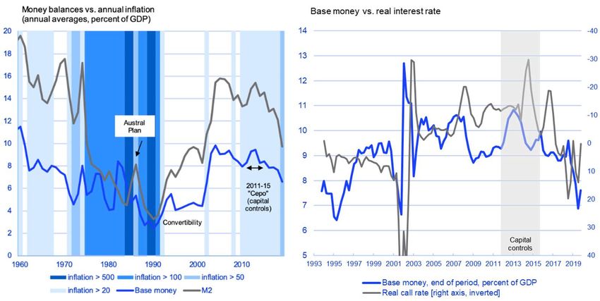
Executive Summary
In this paper, we present our Debt Sustainability Analysis (DSA) considering the available information on the
economic policy framework under the new administration led by President Alberto Fernández. The new
economic program will include measures such as capital controls and incomes policy—often considered
“heterodox” policies. While these measures can be useful, if used properly and judiciously, they should not be a
substitute for a consistent, credible macroeconomic program. A strong fiscal anchor would be critical for the
program’s success. Given the macroeconomic adjustment in 2018-19, the challenge for Argentina is to make
sure the policy effort already undertaken is strengthened and becomes the basis for sustained growth. The high
level of government expenditure should offer plenty of room for savings to achieve a sustainable fiscal position
as an anchor for macroeconomic stability and growth.
Incomes policy, possibly in the form of an “economic-social pact,” could help break price and wage inertia. In
addition to dealing with inflation, a framework for achieving social consensus on needed reforms among all
the social and political stakeholders would be highly desirable. Within this framework, reform of social
security—whose rising deficits have driven the big worsening in the fiscal situation in recent years—should take
center stage to ensure long-term fiscal sustainability. But this would not be enough. Argentina’s decades-long
economic decline shows that other comprehensive, pro-growth reforms are critical. There is now an historic
opportunity to reverse this decline. Our debt analysis is based on the premise that the new administration will
pursue this opportunity and will be successful in restoring growth over the near and medium term.
When measured properly, the burden of public debt as a
share of GDP in Argentina is comparable to that in other
emerging markets and declines over time under a
conservative macroeconomic scenario (chart on the side):
Argentina is not facing an insolvency crisis but a near-term
liquidity crisis, the consequence of having lost market access
as a result of increased policy uncertainty. Argentina’s gross
financing needs in the coming years are comparable to those
of other emerging markets and, policy uncertainty aside,
would be manageable. Therefore, there is a case for
considering a liquidity-based debt restructuring operation.
A debt restructuring operation should not aim to take
Argentina out of debt markets or eliminate dollar shortages
for a sustained period ahead—this is unrealistic as it would be for any other financially integrated, mid-sized
economy. Rather, the goal should be to deal with the near-term liquidity crisis and give the government time
to adopt a credible policy program while the recovery gains momentum and the social consensus for needed
reform is achieved. A positive policy credibility shock could trigger a virtuous cycle that lifts Argentina from its
current crisis. The alternative scenario may result in a vicious cycle in which the recession deepens, inflation
rises, and poverty increases.
2 | PLEASE SEE IMPORTANT DISCLOSURES AT THE END OF THE DOCUMENT.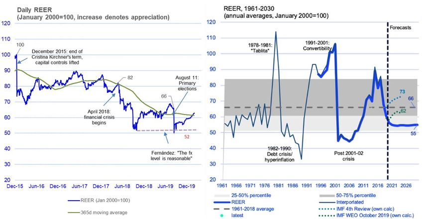
In our view, each stakeholder—the Argentine society and political system, the official creditors, and the private
creditors—can contribute to the solution of the Argentine crisis. A cooperative solution is feasible and would
likely lead to much better economic outcomes for all parties involved. Conversely, it would be unfair to ask
creditors to provide large debt relief in the absence of a credible policy and reform program on the grounds
that Argentina is “insolvent” because its debt is “unpayable.” This would be inconsistent with Argentina’s
economic potential under reasonable policies and the experience of other emerging market countries, including
those that underwent debt restructurings.
Unfair debt restructuring proposals—based on a request for excessive debt relief or including insufficient
policy effort and reform—would likely be rejected. Unfair proposals would create a high risk of Argentina
being unable to access the international capital markets for an extended period, leaving the official sector as
the only provider of external capital. Protracted financial isolation, financial crisis and, in the worst case, debt
default would hardly be the basis for meeting Argentina’s growth objectives.
We believe creditors would not be amenable to any significant changes in contracts without meaningful
steps taken in the critical structural areas, from fiscal to other pro-growth reforms. This is ultimately a
political decision on the path that Argentina should take rather than a capacity-to-pay issue.
This report has been prepared by Autonomy Capital. As of the date of publication of this report, Autonomy Capital and/or
its affiliated or related persons (“Autonomy”) holds positions in or has exposure to sovereign debt issued by Argentina
and/or related financial instruments (“Relevant Instruments”)(whether directly or indirectly). The report may contain
conclusions which would favor the positions in Relevant Instruments held by Autonomy and Autonomy may stand to
realize significant gains (or losses) in the event that the price of one or more Relevant Instruments changes. Autonomy
intends to transact in Relevant Instruments for an indefinite period in the future after the publication of this report, and
as a result its position with respect to Relevant Instruments may change significantly from that held at the time of
publication (including becoming long, short or neutral) regardless of the views stated in this report. Autonomy may not
update this report to reflect changes in positions in Relevant Instruments that may be held by Autonomy from time to
time.
3 | PLEASE SEE IMPORTANT DISCLOSURES AT THE END OF THE DOCUMENT.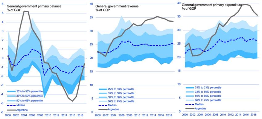
In this paper, we present our Debt Sustainability Analysis (DSA) considering the available information on the economic
policy framework under the new administration led by President Alberto Fernández. In the absence of a comprehensive
policy announcement, our analysis is necessarily based on our interpretation of what we could realistically expect going
forward.
An economic program based on “rational heterodoxy”
We could expect a macroeconomic stabilization and reform program along the following lines:
Monetary and exchange rate policies. Capital controls are expected to remain in place for some time. The
monetary program will aim “to support a reduction in inflation via a prudent management of money supply.” 1
Capital controls provide, in principle, increased domestic autonomy in the conduct of monetary policy. This
should allow for a gradual recovery of real money balances and lower interest rates. Given the objective of
preserving a competitive foreign exchange rate (FX), a managed floating regime would be used to maintain a
stable real effective exchange rate (REER). 2
Incomes policy. Incomes policy, possibly in the form of an “economic-social pact” among different social parts,
would serve as a coordination mechanism to guide prices and wages along a gradual disinflation path.
Government-controlled nominal variables—such as the public tariffs, public wages and pensions would be
managed prudently to help reduce the nominal inertia in the economy and thus strengthen the credibility of
the incomes policy framework program. If well executed and part of a credible program, incomes policy should
provide an additional nominal anchor while permitting some gradual recovery in private real wages from a low
level without triggering a wage-price spiral.
Fiscal policy. Fiscal policy would target the achievement of primary surpluses within a reasonable timeframe.
The fiscal package included in the “Social Solidarity and Productive Reactivation” emergency law passed at the
outset of the Fernández administration is encouraging, even though specific fiscal targets have not been
announced.3 In terms of financing, the budget should receive the transfer of a portion of its seignorage 4
revenue from the central bank.
Structural reforms. An economic-social pact could also be the ideal forum for achieving the social consensus on
the needed growth-enhancing reforms. There could be some changes in labor regulations at the sectoral level,
possibly in conjunction with tax reform to improve economic efficiency and encourage formal employment.
Social security reform would be highly desirable to ensure long-term fiscal sustainability. To attract foreign
investment into the energy sector, especially Vaca Muerta, some special investment regimes could be
introduced—although we believe that macroeconomic stability would be the biggest driver of foreign
investment. Spain’s Toledo Pact aimed at achieving long-term sustainability of social security is a good example
of how to harness social consensus for structural reform in a de-politicized manner. 5
1
http://www.bcra.gov.ar/Pdfs/Institucional/ObjetivosBCRA_2020.pdf
2
http://www.bcra.gov.ar/Noticias/BCRA-fijo-lineamientos-de-pol%C3%ADtica-monetaria270120.asp
3
https://www.clarin.com/economia/emergencia-ajuste-fiscal-podria-rondar-us-6-000-millones_0_Gv5nXim1.html
4
We define seignorage as the increase in base money during a given period needed to maintain a certain level of real money balances. Strictly
speaking, this is a different concept from the central bank’s economic profits, which we also calculate. Relatively high inflation in the coming
years sustain a high flow of seignorage, which in turn generates an economic profit as peso-denominated interest-bearing liabilities are reduced
over time.
5
On the Toledo Pact, see:
https://www.bde.es/f/webbde/SES/Secciones/Publicaciones/PublicacionesSeriadas/DocumentosOcasionales/17/Fich/do1701e.pdf
4 | PLEASE SEE IMPORTANT DISCLOSURES AT THE END OF THE DOCUMENT.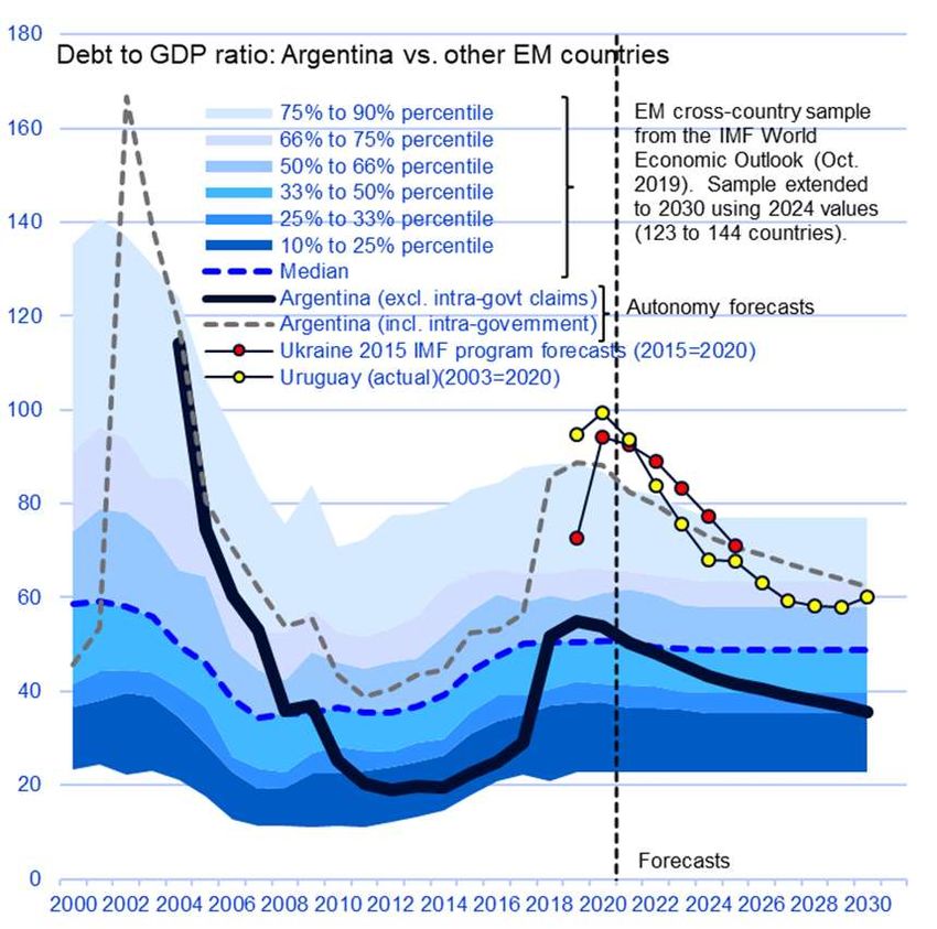
This economic program should provide a policy framework based on “heterodox rationality” that stabilizes the economy
and restarts economic growth. In this regard, there are similarities with the situation in 2002-03, when capital controls
and a managed peg helped stabilize the economy and set the basis for strong recovery, despite initial skepticism. 6 A
successful stabilization program would likely trigger a period of rapid catch up in growth, as in the aftermath of past
successful stabilization programs, allowing Argentina to stop falling behind its regional neighbors (Figure 1). The best-
case scenario is that the heterodox measures open a window of opportunity to stabilize the economy, lower inflation,
and restart economic growth.

            Figure 1: Per capita GDP in constant and dollar terms since 1960

            Sources and notes: Real GDP data from Haver Analytics interpolated with historical data from “PIB Argentina 1900-
            2012: En búsqueda de una tendencia de crecimiento sostenible”, Ariel Coremberg. Mesa Tendencias
            Macroeconómicas 1913-2013: Ariel Coremberg, Adrian Ramos, Pablo Gerchunoff, Daniel Heymann, available at
            https://arklems.org/pbi/. Argentina’s forecasts are based on Autonomy’s base case scenario described in the main
            text. Per capita GDP forecasts for the other countries are from the IMF’s World Economic Outlook (October 2019) as
            reported in Haver Analytics.

In principle, the function of incomes policy in high-inflation situations is that of a nominal anchor that provides a
coordination mechanism to reduce prices and wage inertia along a disinflationary path. 7 By making price and wage
decisions forward-looking, it should reduce the cost of disinflation. The role of the government goes beyond facilitating
negotiations among the price and wage setters. Critically, it should provide a credible macroeconomic framework that is
consistent with and supportive of the disinflation targets. Only within a consistent program can the agents’ expectations

6
  At the time, there were views that the initial stabilization of the Argentine economy was unsustainable and only a “dead cat bounce,” as the
IMF’s Anne Krueger reportedly said
(http://policydialogue.org/files/publications/Argentinian_Debt_History_Default_Damill_Frenkel_Rapetti.pdf). In the event, the economy grew
an average of close to 9% per year between 2003 and 2007.
7
  The adoption of income policy to break price and wage inertia in heterodox stabilization programs has historical precedent, such as in
Argentina (Plan Austral), Brazil and Israel in the 1980s. The evidence from these programs is that they were initially successful in lowering
inflation. However, they failed subsequently when the initial success in lowering inflation was not matched by a permanent adjustment in
policies, with the fiscal deficit often rising again soon after the start of the program. Other examples of successful economic-social pacts are
Sweden in the 1930s and Australia in the 1980s. See R. Dornbusch and M. H. Simonsen, “Inflation Stabilization: The Role of Incomes Policy and
of Monetization”, in R. Dornbusch, “Exchange Rates and Inflation”, The MIT Press, 1988; and “Inflation Stabilization: The Experience of Israel,
Argentina, Brazil, Bolivia, and Mexico”, edited by M. Bruno, G. Di Tella, R. Dornbusch and S. Fischer, The MIT Press, 1988. Also,
https://www.clarin.com/opinion/condiciones-acuerdo-economico-social-viable_0_OPuoR0a5.html.

5 | PLEASE SEE IMPORTANT DISCLOSURES AT THE END OF THE DOCUMENT.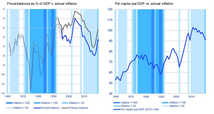
of lower inflation be met and in turn permit a gradual recovery of real wages without triggering a price-wage spiral. The
lesson from history is that incomes policy can help lower inflation quickly but, for long-lasting success, it is not a
substitute for a consistent macroeconomic program. Our base case scenario is built on the assumption that a credible
gradual disinflation path will manage to bring annual inflation from above 50% in 2019 to the low 40s in 2020 and then
to middle double digits in 4-5 years.
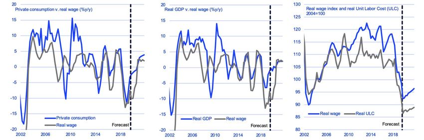
Along with incomes policy, capital controls should create room for lowering real interest rates while avoiding large FX
fluctuations and maintaining a level of the REER that is supportive of external surpluses. Capital controls allow, in
principle, for reducing domestic interest rates below the level that would be needed for external equilibrium in their
absence. A (partially) closed capital account should also allow for gradual remonetization of the economy after the sharp
fall in real money balances during the last two years (Figure 2, left chart) as the range of foreign-based investment
options for allocating domestic savings is reduced—this happened during the early part of the capital control period of
2011-15. Remonetization would likely increase further if inflation is successfully reduced over time.
Figure 2: Real money balances, inflation, and real interest rates
Sources: Argentine Statistical Agency (Indec); Haver Analytics; and Autonomy calculations. Real rates are based on realized
annual inflation.
Monetary policy under the IMF program was guided during most of 2019 by a “zero-monetary-base-growth” target and
resulted in falling real money balances and high real interest rates (Figure 2, right chart). However, little progress was
made in reducing inflation, which was single-handedly the biggest disappointment under the IMF program. 8 The new
economic program will initially rely on incomes policy as a coordination mechanism for wage and price decisions.
Monetary aggregate targets will remain a nominal anchor in the program, although not the only ones in the initial stages.
The policy challenge will be to use the increased flexibility in monetary policy with moderation; it is encouraging in this
regard that the central bank has explicitly committed to avoiding negative real interest rates. 9 The monetary program in
our base case scenario shows a very gradual recovery in real base money over time—monetary base as a share of GDP
8
The IMF forecast for annual CPI inflation in 2019 went from 20.2% in the Staff Report for the Second Review (December 2018) to 40.2% in the
Staff Report for the Fourth Review (July 2019).
9
http://www.bcra.gov.ar/Noticias/BCRA-fijo-lineamientos-de-pol%C3%ADtica-monetaria270120.asp.
6 | PLEASE SEE IMPORTANT DISCLOSURES AT THE END OF THE DOCUMENT.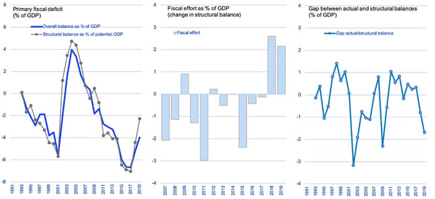
recovers to its 2018 level only in 2028.10 As shown below, this is internally consistent with a reduction in the central
bank’s peso-denominated interest-bearing liabilities and the sustainability of its capital over time, even after including
the transfer of a portion of seignorage to the government. The reason being that, starting gradual disinflation from
today’s inflation level, the amount of seignorage is significant even at the current level of real money balances.

                                 Figure 3: REER from a long-term perspective

     Sources and notes: The REER is calculated on data from the Central Bank of the Republic of Argentina as reported in Haver Analytics. The
     earlier data is from J. L. Espert and G. Vignoli, “Tipo de Cambio Real de Largo Plazo en Argentina: 1961-2017”, CEMA Working Paper 60, 2018
     (https://ucema.edu.ar/publicaciones/download/documentos/630.pdf). The chart also shows Autonomy’s forecast for the base case
     scenario described below, and Autonomy’s estimates of the REER path included in the IMF Staff Report for the Fourth Review
     (https://www.imf.org/en/Publications/CR/Issues/2019/07/15/Argentina-Fourth-Review-under-the-Stand-By-Arrangement-Request-for-
     Waivers-of-Applicability-47116) and World Economic Outlook (October 2019) database as reported in Haver Analytics, based on the
     published information.

The central bank will also seek to preserve a competitive FX level—the exact level has not been specified—within a
regime of managed FX float.11 In our base case scenario, the REER stays in the medium-term at a level between the low
reached after the August 2019 election—when then-candidate Fernández said that the FX was competitive 12—and its
levels in the initial phase of the Fernández administration (Figure 3, left chart). Our base case therefore includes a margin
for additional real depreciation from current levels and is competitive from a long-term perspective (Figure 3, right
chart); only twice since the early 1960s has the REER been lower for a sustained period. Our medium-term REER
assumption is also significantly below the IMF’s two most recent publicly available forecasts, both shown in the chart. 13
Our goal is not to make our debt analysis reliant on an appreciating real exchange rate, even though in a successful
stabilization there would likely be room for some real appreciation (see Annex A for two additional REER valuations that
reach a similar conclusion).

10
   The assumed recovery in real money balances is broadly consistent with maintaining positive real interest rates and a demand for money
with a moderate (semi) interest elasticity of -0.2.
11
   http://www.bcra.gov.ar/Pdfs/Institucional/ObjetivosBCRA_2020.pdf, and http://www.bcra.gov.ar/Noticias/BCRA-fijo-lineamientos-de-
pol%C3%ADtica-monetaria270120.asp.
12
   https://www.lanacion.com.ar/politica/alberto-fernandez-el-dolar-60-esta-valor-nid2277730
13
   These are the forecast in the IMF Fourth Review Staff report published just before the August 2019 election and the forecast in the October
2019 World Economic Outlook. Both paths shown in the chart are our own calculations for the REER based on the publicly available
information.

7 | PLEASE SEE IMPORTANT DISCLOSURES AT THE END OF THE DOCUMENT.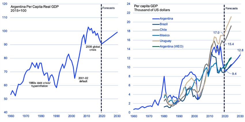
In the end, a credible path to fiscal primary surpluses needs to be the anchor for any sustainable economic program. The
fiscal anchor was progressively lost under the subsequent Kirchner governments during 2003-15, especially after the
2005 debt restructuring was finalized. While government revenue rose significantly, this was more than offset by rising
government expenditure. As a result, the general government’s primary balance sank 10% of GDP from a surplus of more
than 5% of GDP under the administration of Nestor Kirchner—in which Fernández served as Chief of Cabinet—to a
primary deficit of almost 5% of GDP in 2015, the last year of Cristina Kirchner’s second presidential term (Figure 4).
During this time, Argentina’s government expenditure as a share of GDP rose starkly above levels in other Emerging
Market (EM) economies, almost doubling from the early years of the previous decade. The process of reducing this
enormous deficit started under the Macri administration and accelerated in 2018-19 after the financial crisis cut off
market access. Overall, this adjustment brought the federal primary deficit to 0.4% of GDP in 2019. 14

           Figure 4: Argentina’s fiscal numbers in international perspective

     Sources and notes: IMF’s World Economic Outlook database as reported in Haver Analytics; and Autonomy calculations. The cross-
     country distribution is based on the sample of emerging and developing countries included in the IMF’s World Economic Outlook
     database (October 2019) as reported in Haver Analytics. The cross-country sample includes between 131 and 144 countries
     depending on data availability.

According to our debt analysis, a federal primary surplus of about 1% of GDP—not including seignorage revenue from
the central bank—would put the federal debt-to-GDP ratios on a declining path over time under our base case scenario. 15
This amounts to reverting part of the big fiscal deterioration observed during the last few years, especially the second
administration of Cristina Kirchner (2011-15). This level of primary surpluses would not be extraordinary among EM
economies, but it would still be short of the level in EM countries that completed debt restructurings (see below). It
would be unrealistic to ask creditors for major debt relief without Argentina making what, in relation to its own relatively
recent history and international experience, looks like a manageable effort. Moreover, the very large government
expenditure should undoubtedly provide wide-ranging scope for spending rationalization and savings at all levels of
government. Annex B presents additional discussion on possible fiscal savings.

Importantly, Argentina made a significant fiscal effort over the last two years that offers a good starting point to move
forward. Based on the IMF’s estimates in its October 2019’s World Economic Outlook, the “structural” fiscal balance—

 https://www.argentina.gob.ar/noticias/sector-publico-nacional-no-financiero-ejecucion-base-caja-2019
14

 In its Fourth Review under the current Stand-by Arrangement, the last prior to the PASO, the IMF forecasted the primary surplus at 1.0% of
15

GDP in 2020-23, rising to 1.4% in 2024, the last year of the forecast horizon. No seignorage revenue was included in the debt forecast.

8 | PLEASE SEE IMPORTANT DISCLOSURES AT THE END OF THE DOCUMENT.
which corrects for the effect of the business cycle on the fiscal balance—improved by about five percentage points of
GDP over 2018-19, a sizeable fiscal effort after several years of growing structural deficits (Figure 5, left and middle
charts). This adjustment was rapid and pro-cyclical, as it took place while the economy was contracting. As a result, the
gap between the actual and structural deficits was close to 2% of GDP in 2019 (Figure 5, right chart). In other words,
were the economy able to close its large output gap—about 5% using a simple rule-of-thumb calculation—the
improvement in the fiscal balance would be close to 2%, pushing the primary balance to about 1% of GDP, a level
compatible with long-term fiscal sustainability.

                                     Figure 5: Structural fiscal balances

       Sources and notes: Autonomy calculations on data from the IMF World Economic Outlook (October 2019) as reported in Haver
       Analytics.

Seen in this light, the Fernández administration’s insistence on restoring growth as a condition for additional fiscal
adjustment is understandable—a recovery would indeed go a long way toward further improving the fiscal accounts.
However, this analysis also underscores the importance of creating the conditions for a prompt recovery, which in our
view depends heavily on restoring policy credibility and the confidence of economic agents. Thus, the policy emphasis
should be on reforms that strengthen the confidence in the medium-term fiscal framework, the only solid anchor for the
other components of the economic program. If this could be done, there would be less urgency to deliver additional pro-
cyclical fiscal tightening in the near term. Increasing long-term credibility, reforms that address long-term imbalances—
such as in the social security system—would be especially beneficial and would reduce the urgency of front-loaded fiscal
measures. In a country whose estimated per capita real GDP in 2019 is below its 2007 level, there is not much room left
for stop-gap measures.

Ultimately, the success of the new administration’s policies will stem from the consistency and credibility of the overall
macroeconomic program. The heterodox policies can only be effective as temporary measures and should not be a
substitute for a consistent medium-term macroeconomic framework. In fact, failing to take advantage of the success in
early stages of stabilization to implement politically costly fiscal adjustment is the typical mistake that leads to the failure

9 | PLEASE SEE IMPORTANT DISCLOSURES AT THE END OF THE DOCUMENT.
of heterodox stabilization programs.16 The longer-term cost of heterodox policies should also be considered. It is difficult
to expect stronger medium-term growth if intrusive capital controls remain an open-ended feature of the economy.

The Fernández administration has a historical opportunity to achieve the social consensus in support of the policies and
reforms needed for sustained growth to benefit the entire society. The risk is that these heterodox features weigh
further on economic efficiency and exacerbate the economy’s existing structural weaknesses. Encouragingly, President
Fernández himself has emphasized the importance of macroeconomic order as a basis and necessary condition for
economic development, promising the consistency of his economic plan. 17 Argentina’s own economic history is a clear
reminder that macroeconomic policy volatility, especially high fiscal deficits, is a harbinger of macroeconomic crisis and
dismal economic performance rather than a source of positive economic stimulus (Figure 6). Our base case scenario is
built on the premise that the new administration’s economic program will be successful in achieving fiscal and monetary
order and that this will sustain at least some moderate growth in the medium term.

          Figure 6: Fiscal balances, inflation and per capita real GDP since 1960

     Sources and notes: The fiscal balances are from the Argentine Minister of Finance; earlier data is from O. Cetrangolo, J.P. Jimenez, 2003,
     “Política fiscal en Argentina durante el regimen de convertibilidad”, Cepal, available at
     https://repositorio.cepal.org/bitstream/handle/11362/7288/1/S034252_es.pdf). The inflation data is from the Argentine Statistical Agency
     (INDEC). Per capita Real GDP is calculated using data from Haver Analytics and the World Bank’s World Development Indicators as reported
     in Haver Analytics. The older real GDP data is from “PIB Argentina 1900-2012: En búsqueda de una tendencia de crecimiento sostenible”,
     Ariel Coremberg. Mesa Tendencias Macroeconómicas 1913-2013: Ariel Coremberg, Adrian Ramos, Pablo Gerchunoff, Daniel Heymann,
     available at https://arklems.org/pbi/;

How an economic recovery could look in the near term: virtuous vs.
vicious cycles
If this economic program is implemented with enough credibility to re-establish the confidence of economic agents, we
expect a recovery to take place during 2020 and gain strength during 2021. Our base case macroeconomic scenario is

16
   “Inflation Stabilization: The Experience of Israel, Argentina, Brazil, Bolivia, and Mexico”, edited by M. Bruno, G. Di Tella, R. Dornbusch and S.
Fischer, The MIT Press, 1988.
17
   https://www.clarin.com/politica/asuncion-alberto-fernandez-discurso-completo-nuevo-presidente_0_FXJxjVYE.html

10 | PLEASE SEE IMPORTANT DISCLOSURES AT THE END OF THE DOCUMENT.
consistent with, and supported by, the economic program we have described. This scenario is based on the notion that
policy credibility is rebuilt slowly initially but that it successfully reactivates at least moderate growth over time.
Incomes policy can be instrumental in creating the conditions for economic recovery in the near term. Past recessions in
Argentina typically ended when real wages stopped falling and began recovering, pulling up consumption and real GDP
growth (Figure 7, left and middle charts). At the current point in the economic cycle, there should be enough room for
accommodating a gradual recovery in real wages, given that their precipitous downward fall in recent quarters was likely
an over-reaction to disruptive FX depreciation and the resulting jump in inflation. In fact, real wages are now estimated
to be back to their 2003 level and real unit labor costs well below their 2002 level (Figure 7, right chart). This
overshooting in wages provides the basis for an economic-social pact to accommodate a gradual recovery in private real
wages without endangering competitiveness or fueling a wage-inflation spiral.
Figure 7: Private consumption, real GDP, and real wage indicators
Sources and notes: Haver Analytics and Autonomy calculations and forecasts based on the base case scenario described in the main text.
Our near-term base case scenario is built on the premise that a growth recovery is sustained initially by a gradual rise in
real wages, with the additional support of the short-term measures aimed at low-income sectors included in the
December recovery package. The main drivers of growth during the next two years could be as follows (see Figure 8,
table and charts, for a numerical illustration of this scenario):
Private consumption is driven by a recovery in real wages in the context of the economic-social pact, with
moderate year-on-year growth in 2020 (about 2%) after a contraction of more than 20% during 2018-19. As
typical in recoveries, private sector employment growth picks up only with a lag once economic activity gains
some momentum. Public consumption remains on a declining path.
Investment stays soft initially as the new economic program gains traction. The recovery in investment from
the second half of 2020 is modest compared to past recoveries.
Net exports remain the main growth driver in 2020. Exports grow moderately going forward at an annual pace
of 2%, roughly the average since 2005. On the other hand, imports continue contracting during the first half of
2020 until domestic demand stabilizes. Once the latter bottoms out and starts growing during the year, net
exports gradually fade as a growth driver.
11 | PLEASE SEE IMPORTANT DISCLOSURES AT THE END OF THE DOCUMENT.This outlook leads to annual average growth of zero in 2020, interrupting two years of negative growth. 18 By design, this is a conservative scenario, with better economic outcomes more likely in our view if the economic program is credibly implemented and uncertainty about the debt situation is efficiently resolved. Specifically, compared to previous recessions, our base case is built on a slow recovery in real wages—and therefore private consumption—and investment. If policy manages to create a positive credibility shock, there could be a much faster rebound in investment as a growth driver, which would trigger a virtuous growth cycle in which real wages and consumption can grow much faster. The international evidence from past debt restructurings reviewed below shows that these are typically followed by stronger policies—in the form of higher fiscal surpluses—and significant increases in investment-to-GDP ratios as drivers of stronger post-restructuring growth. A similar virtuous growth cycle could be triggered in Argentina, but only if policymakers take the lead by sending strong, concrete signals on policy direction. In our base scenario, this positive confidence shock is the main driving force behind the near-term rebound in 2020-21 as it creates the conditions for a non-inflationary recovery in real wages—and hence consumption—and a moderate recovery in investment. Conversely, failure to generate a positive confidence shock could lead to the opposite outcome, namely a vicious growth cycle led by further declines in investment, real wages, employment and consumption—in a second contraction leg reminiscent of the 2001-02 deep dive after several quarters of recession. The international evidence also suggests that the approach to debt restructuring could have a significant impact on the post-restructuring behavior of the real economy, with significant divergence between market-friendly restructurings and those that involve defaults. Therefore, what path Argentina takes will be intimately linked to the strength of the policy framework and the approach to debt restructuring. 18 Our forecast for 2020 is above the median expectation in the latest central bank’s expectations survey, which puts growth in 2020 at -1.5% (http://www.bcra.gov.ar/Noticias/REM-enero-20.asp). This expectation is in turn considerably worse than the statistical carryover from 2019, which, based on our calculations on the seasonally adjusted real GDP data as provided in Haver Analytics, is 0.0% considering only the available GDP data through Q3, or -0.5% if we include negative growth in 2019Q4 in line with consensus expectations (-0.7%). In other words, the consensus forecast assumes that the economy’s contraction will continue through 2020. Our base case scenario assumes that this outcome could be avoided if there were a positive credibility shock that led to a quick resolution in the uncertainty surrounding the debt situation. 12 | PLEASE SEE IMPORTANT DISCLOSURES AT THE END OF THE DOCUMENT.
Figure 8: An illustrative recovery scenario in 2020-21
Growth forecasts 2018 2019 2020
P ercentage changes unless no ted o therwise f orecast s f orecast s
2004 2005 2006 2007 2008 2009 2010 2011 2012 2013 2014 2015 2016 2017 2018 2019 2020 2021 Q1 Q2 Q3 Q4 Q1 Q2 Q3 Q4 Q1 Q2 Q3 Q4
Real GDP 8.4 8.9 8.0 9.0 4.1 -5.9 10.1 6.0 -1.0 2.4 -2.5 2.7 -2.1 2.7 -2.5 -2.5 0.0 2.0 0.0 -5.0 -0.2 -1.2 -0.1 -0.7 0.9 -0.3 -0.9 0.5 0.6 0.6
q4/q4 -6.4 -0.2 0.8 2.0
Domestic demand 13.3 9.1 9.3 11.3 6.9 -7.9 14.2 10.2 -1.3 4.0 -3.9 4.2 -1.6 6.0 -3.4 -8.4 -1.0 2.8 -1.7 -3.6 -3.3 -6.0 -0.8 -1.1 0.8 -0.8 -1.3 0.4 0.5 0.7
q4/q4 -13.8 -1.9 0.3 3.1
contributions to growth 11.9 8.4 8.6 10.7 6.6 -7.8 13.8 10.2 -1.4 4.2 -4.1 4.4 -1.7 6.4 -3.8 -9.2 -1.0 2.8
Private consumption 10.7 7.4 11.0 9.3 7.2 -5.4 11.2 9.4 1.1 3.6 -4.4 3.7 -0.8 4.0 -2.4 -6.4 -0.9 3.4 1.9 -4.4 -4.3 -2.2 -1.4 0.0 0.3 -1.2 -0.9 0.3 0.6 0.9
q4/q4 -8.8 -2.3 0.9 3.8
Public consumption 2.6 9.9 3.7 7.8 5.0 5.6 5.5 4.6 3.0 5.3 2.9 6.9 -0.5 2.7 -3.3 -0.9 -3.4 -2.4 -2.4 -0.6 -1.5 -0.8 1.6 -0.9 -0.1 -1.0 -1.0 -1.0 -1.0 -0.5
Gross fixed capital investment 35.3 15.8 14.5 20.5 8.7 -22.6 26.3 17.4 -7.1 2.3 -6.8 3.5 -5.8 12.2 -5.7 -14.4 -0.7 3.5 -0.3 -8.0 -8.0 -10.0 -0.9 0.3 0.0 -1.0 -0.5 0.0 0.5 1.0
q4/q4 -24.1 -1.5 1.0 4.1
Net exports (contributions to growth) -3.5 0.4 -0.6 -1.6 -2.6 1.9 -3.6 -4.2 0.3 -1.8 1.6 -1.7 -0.4 -3.7 1.3 6.6 1.0 -0.8 1.9 -1.0 3.4 5.3 0.8 0.4 0.1 0.5 0.4 0.2 0.0 -0.1
Exports 7.3 12.9 5.6 8.2 0.7 -9.3 13.9 4.1 -4.1 -3.5 -7.0 -2.8 5.3 1.7 -0.7 8.2 2.5 2.0 7.1 -13.2 3.0 11.7 1.0 -0.4 2.0 0.5 0.5 0.5 0.5 0.5
Imports 40.5 15.8 11.0 19.6 13.6 -18.4 35.2 22.0 -4.7 3.9 -11.5 4.7 5.8 15.4 -4.7 -17.0 -1.7 5.1 -1.5 -5.5 -9.2 -10.8 -2.2 -1.9 1.3 -1.4 -1.1 -0.2 0.4 1.0
Real wage bill 13.2 13.4 13.8 9.0 2.1 0.4 2.4 7.5 2.8 0.3 -3.4 3.4 -5.7 4.1 -6.4 -12.3 -5.9 3.1 -1.9 -2.3 -6.7 -4.6 -0.4 -3.0 -2.2 -6.5 0.2 0.5 0.2 1.1
q4/q4 -14.7 -11.7 2.0 3.4
Employment 6.8 8.9 7.7 5.8 4.6 -1.6 2.3 3.4 0.4 -0.1 0.2 0.2 -0.1 0.9 -0.2 -2.4 -0.6 0.8 -0.1 -0.3 -0.7 -0.9 -0.5 -0.6 -0.6 0.0 0.1 -0.1 -0.2 0.1
q4/q4 -2.0 -1.7 -0.2 1.4
Real wage 6.1 4.1 5.7 3.1 -2.4 2.0 0.0 4.0 2.4 0.5 -3.5 3.2 -5.5 3.2 -6.3 -10.2 -5.3 2.2 -1.8 -2.1 -6.1 -3.7 0.1 -2.4 -1.7 -6.4 0.2 0.6 0.4 1.0
q4/q4 -13.0 -10.2 2.2 2.0
Unit real labor cost (June '18=100) 1/ 92 99 103 99 104 103 99 102 101 102 100 103 98 99 90 80 81 82 97 100 94 90 90 88 85 80 81 81 80 81
1/ End-period values.
Real GDP and private consumnption Real GDP in past recessions Real GDP grow th v. real w age index/real ULC Investment in past recessions
Real GDP v. Net exports (%y/y)
(log of 2004 prices) (last quarter bef ore recession=100) (last quarter before recession=100)
7.0 6.5 120 1995 15 130 15 140
2002
115 1995
Real GDP 2008 10
6.8 6.3 10 120 120 2002
110 2012 2008
Private consumption
[right] 2014 5 2012
6.6 6.1 105 5 110 100 2014
2016 2016
100 2020 0 2020
6.4 5.9 0 100 80
95
-5
90
6.2 5.7 -5 Real GDP (%y/y) 90 60
-10
85 Real wage [right] Real GDP
6.0 5.5 Real ULC [right] Net exports contrib.)
80 -10 80 -15 40
1993 1997 2001 2005 2009 2013 2017 2021 1 3 5 7 9 11 13 15 17 19 2003 2007 2011 2015 2019 1 3 5 7 9 11 13 15 17 19
1993 1997 2001 2005 2009 2013 2017 2021
Real GDP v. employment (%y/y) Consumption in past recessions
Real GDP and investment (log of 2004 prices) Private consumption v. real w age bill (%y/y) Domestic demand v. imports(%y/y)
(last quarter before recession=100)
7.0 5.2 15 20 Private consumption 15 45 115
Real GDP Real GDP Real wage bill 1995
5.0 35 2002
Employment 15 10
6.8 Investment [right]
10 25 2008
4.8 105
10 2012
5 15
4.6 2014
6.6 5 5 5 2016
4.4 0 95 2020
0 -5
6.4 4.2 0
-5 -15
-5
4.0 85
6.2 -25
-5 -10
3.8 -10
Domestic demand Imports [right scale] -35
6.0 3.6 -10 -15 -15 -45 75
1993 1997 2001 2005 2009 2013 2017 2021 2003 2007 2011 2015 2019 2003 2007 2011 2015 2019 1993 1997 2001 2005 2009 2013 2017 2021 1 3 5 7 9 11 13 15 17 19
Sources and notes: Autonomy forecasts and calculations. Historical data is from Haver Analytics.
13 | PLEASE SEE IMPORTANT DISCLOSURES AT THE END OF THE DOCUMENT.The challenge of achieving sustained growth over time Turning a near-term rebound into sustained growth will require addressing the root causes of Argentina’s economic secular decline. While well-known, and deeply saddening, it is worth recalling Argentina has experienced a significant decrease in its international ranking over several decades. The divergence in economic performance compared to the other economies in the same region is stunning (Figure 9, left chart). Not only did Argentina grow much less on average, its growth was marked by extreme boom-bust cycles, with every single crisis in the last decades creating a long-lasting negative drag and leading Argentina to fall further behind. Its enormous policy volatility over the past decades has likely been one of the core reasons behind Argentina’s underperformance (Figure 9, right chart). A sustainable policy framework that leaves behind policy volatility would probably go a long way in creating the conditions for sustained, if not spectacular, economic growth. Conversely, another extended debt crisis would bode poorly for future growth. Figure 9: Argentina’s secular economic decline and economic policy volatility Real GDP per capita (2011 US dollars) (in logs, 1950=100) Economic policy volatility vs. economic convergence Sources and notes: The left chart is based on Autonomy calculations using data from the Maddison Project Database, version 2018. Bolt, Jutta, Robert Inklaar, Herman de Jong and Jan Luiten van Zanden (2018), “Rebasing ‘Maddison’: new income comparisons and the shape of long-run economic development” Maddison Project Working Paper, nr. 10, available at www.ggdc.net/maddison. The right data is from Oscar Calvo-González, Axel Eizmendi, and Germán Reyes, 2018, “Winners Never Quit, Quitters Never Grow”, World Bank Working Policy Paper 8310 available at http://documents.worldbank.org/curated/en/634591516387264234/pdf/WPS8310.pdf. Going above moderate growth—and thus making a true difference to standards of living—will require tackling Argentina’s institutional deficiencies. Argentina’s “growth environment index”—a summary measure of institutional indicators that are found to correlate with growth performance across countries—declined significantly between the early 2000s to the middle of the last decade, before recovering in more recent years (Figure 10, left chart); this caused Argentina to lose several positions in international rankings, starting from an already weak position, and to fall toward the bottom of a sample of 55 of the more developed economies in the world. Consistently with anecdotal accounts, the decline in institutional quality was concentrated in the quality of the business environment, an area that encompasses features such as ease of doing business; political and judicial corruption; rule of law; and the role of the government in the economy (Figure 10, right chart). While a detailed analysis of institutional reform is beyond the scope of this paper, there is no question that an overhaul of Argentina’s institutions should be a high priority for any growth-oriented policymaker. 14 | PLEASE SEE IMPORTANT DISCLOSURES AT THE END OF THE DOCUMENT.
Figure 10: Institutional Quality in Argentina

 Sources and notes: Data based on Autonomy research. The Growth Environment Index is based on a cross-country panel regression of long-
 term growth on Institutional Quality variables and other growth drivers. The institutional variables are as follows. Political Inclusion:
 Democracy Indicators from V-Dem, a political science project from the University of Gothenburg; World Governance Indicators from the
 World Bank (WB). Business Environment: Ease of doing business (WB), Political Corruption and Judicial Corruption (V-Dem), Rule of Law data
 (V-Dem and WB), Trade Freedom, Regulation and Government Size data from Fraser Institute. Human Capital: Education data from U.N.
 Development Report, Life Expectancy data from U.N. Population Statistics. Technology: ICT (e.g. Individuals using internet or mobile subs)
 and innovation data (e.g. patents, researchers in R&D) from World Development Indicators.

In terms of medium-term growth beyond 2021, our base case scenario assumes conservatively steady annual growth at
2%. We believe that this modest pace of growth can be achieved if, at very least, macroeconomic order is maintained.
We reiterate, however, that it would be desirable that well-targeted institutional reforms addressed the key institutional
deficiencies in the economy in order to raise potential growth to much higher levels. Our base case is unambitious from a
historical perspective as well. Average annual growth was around 3% or higher in five of the last seven decades, although
with a high volatility (Figure 11, left chart). Growth fell below this level for a sustained period only during the debt
crisis/hyperinflation of the 1980s, and in the most recent decade spanning the last Kirchner and Macri administrations.
Beating the dismal performance of the last decade is not setting the bar very high at all.

In our base case scenario, the coming recovery would be much shallower than in the last two long expansions during the
1990s and 2000s which both followed protracted growth declines (Figure 11, right chart). In this sense, achieving at least
a 2% annual growth in the next few years as assumed in our base case scenario should be achievable if the policy
framework is sound. For comparison, in its latest review (completed in July 2019) the IMF assumed growth of about 3.5%
in the medium term, implying that our assumption incorporates quite a buffer against growth underperformance. The
historical experience of countries exiting debt restructurings discussed below suggests that our base case assumption is
indeed conservative, and that a successful solution to the debt problem would likely trigger higher growth than assumed
here, especially if accompanied by institutional reform.

15 | PLEASE SEE IMPORTANT DISCLOSURES AT THE END OF THE DOCUMENT.
Figure 11: Long-term growth performance and growth
                       recoveries in successful stabilization programs

     Sources and notes: See notes to Figure 1 for sources on real GDP data. The recovery episode from 2020 is based on our base case
     scenario described below.

External balances
Owing to a competitive FX and still soft growth in the near term, our macroeconomic scenario should sustain current
account surpluses of significant magnitude for some time (Figure 12, left chart; these surpluses are measured on a cash
basis)—even though multiple FX and capital controls make forecasting external balances much more complex than usual.
The first implication is that current account surpluses will generate an inflow of dollars that could be available, at least in
part, for debt service payments (more on this below).

                            Figure 12: Sectoral balances and capital flight

          Sources and notes: Central bank of the Republic of Argentina; Argentine Ministry of Finance; Haver Analytics; and
          Autonomy calculations and forecasts under the base case scenario described in the main text.

16 | PLEASE SEE IMPORTANT DISCLOSURES AT THE END OF THE DOCUMENT.
Second, the combination of positive current account surpluses and deficits for the federal government implies that the
private sector, defined here as the residual sector, would be running large cash surpluses—about 7% of GDP in 2020. By
design, the capital controls should hamper the exit of these surpluses in the form of capital flight as happened in recent
years—capital flight reached $27 billion in 2018 and was on course to exceed this number in 2019 before capital controls
were introduced (Figure 12, right chart). With diminished capital flight, there will be a surplus of domestic savings in
search of domestic uses. The domestic debt market is a natural destination for these savings.
This observation brings us to reiterate a point we have already made: the problem Argentina is facing is no longer the
result of existing macroeconomic imbalances, as was the case in the run-up to the 2018 financial crisis. These domestic
savings will be available because a rebalancing in the economy has already taken place. The main problem today is the
lack of policy credibility; its solution requires a strong policy program. This is the pre-condition for dealing with the
liquidity crisis and restarting economic growth.
IMF program
As Argentina’s largest creditor, we expect the IMF will continue to play a role in Argentina. In our base case scenario, we
assume a new IMF program is approved in support of the Fernández administration’s policy framework described above.
The new program provides new financing in the form of $9 billion during 2020-21—corresponding to about three-
quarters of the undisbursed amounts under the current Stand-By Arrangement (SBA)—and additional disbursements
during 2022-23 representing a 75% rollover of the principal repayments to the IMF in those years. This financing is
assumed to be provided under an Extended Fund Facility (EFF) arrangement, which entails longer repayment periods
than under SBA terms and thus stretches out repayments to the IMF over time (Figure 13). 19
The IMF financing in our base case scenario illustrates how the IMF could support a consistent medium-term program. In
our view, a successful stabilization of the Argentine economy requires coordinated participation of the three main
parties directly involved—the Argentine government, the private creditors, and the IMF—and this type of program
would represent the IMF’s contribution to a cooperative solution. We have already described the type of policy
adjustment that could be reasonably expected from the Argentine government. We will describe below the type of
contribution from private bondholders that could support this outcome.
19
https://www.imf.org/en/About/Factsheets/Sheets/2016/08/01/20/56/Extended-Fund-Facility
17 | PLEASE SEE IMPORTANT DISCLOSURES AT THE END OF THE DOCUMENT.Figure 13: Illustrative scenario on a new IMF program
Sources and notes: https://www.imf.org/external/np/fin/tad/extforth.aspx?memberkey1=30&date1key=2019-10-
31&category=forth&year=2019&trxtype=repchg&overforth=f&schedule=exp&extend=y; and Autonomy forecasts under
the base case scenario described in the main text. Net disbursements are the difference between new disbursements and
amortizations.
Debt dynamics under our base case scenario: not an insolvency crisis
Table 1 summarizes the main assumption underlying our base case scenario for our debt sustainability analysis. This base
case is meant to be a conservative yet feasible scenario: growth is assumed to rebound from 2021 and stabilizes at 2%
annually in future years; the REER converges to a competitive level; and the primary balance converges to 1% of GDP.
Our scenario also includes the transfer to the government of a portion of the central bank’s seignorage revenue in a way
that is sustainable for the central bank’s balance sheet, as we discuss below.
Regarding market access, our base case scenario assumes one third of dollar amortizations are rolled over into new
dollar debt and that any remaining financing gap is filled with the issuance of new peso debt. Our approach is to
calculate the borrowing needs that close the financing program and assess whether the resulting amount is realistic. In
terms of borrowing costs, the new dollar debt carries a coupon rate of 8%. This yield level seems broadly in line with
external credit spreads in the aftermath of successful debt restructurings (Figure 14, left chart) and would be at the top
of single-B rated sovereign EM credits (Figure 14, right chart). The new peso debt is inflation-linked and pays—after a
two-year transition period—a real rate of 4%, which would be consistent with a successful stabilization program. 20
Initially, the new debt has short maturities (one and two years), with longer maturities up to ten years in later years. For
simplicity, these interest rates are maintained through the entire forecast period; given that debt ratios decline over
time, this is indeed a conservative assumption.
20
The real yields (as reported in Bloomberg) on the inflation-linked discount bonds maturing in 2033 were at around 4% before the onset of the
financial crisis in 2018. Given our assumption that the maturities would be much shorter, our assumption seems justified under our base case
scenario.
18 | PLEASE SEE IMPORTANT DISCLOSURES AT THE END OF THE DOCUMENT.Table 1: Summary of Macroeconomic Assumptions
-2.5% in 2019
Real GDP growth 0% in 2020.
Stays at 2.0% from 2021.s
Falls gradually to under 30% in 2022, middle double digits from
GDP deflator inflation (annual average) 2025
Average annual trading partners’ inflation is 2.5%
converges to 55 (about 15% below the pre-August 2019 primary
REER (Jan 2000=100)
election level)
Fiscal primary balance as % of GDP -1.0% in 2019; -0.5% in 2020; stays at 1.0% from 2022
Real base money Recovers slowly to 9.8% of GDP in 2028 from 8.8% at end-2019.
Central bank’s budgetary transfers Transfers 1/2 of seignorage revenue to the government budget
(seignorage) Retains all the other accounting profits
No new disbursements under the current SBA
New EFF program in 2020-23:
$9 billion in 2020-21 (corresponds to about 75% of undisbursed
IMF program and other official loans
amount under current SBA)
$27 billion during 2022-23 (75% of maturing amortizations)
Other official disbursements of $3 billion per year
8.0% on dollar debt; 4.0% on real peso debt after a two-year
Interest rate on new market debt
transition
One-third of dollar-denominated debt amortizations are rolled
Market access over into new dollar debt
Peso debt fills the remaining financing needs
Automatically rolled over under unchanged terms
Intra-government debt
Interest is capitalized; capitalized interest accrues interest
19 | PLEASE SEE IMPORTANT DISCLOSURES AT THE END OF THE DOCUMENT.Figure 14: Exit yields in selected restructurings
and yields in single-B sovereign EM credits
Sources: Haver Analytics and Bloomberg. EM yields on December 31, 2019.
Figure 15 shows the DSA results under our base case scenario. 21 Total federal debt starts from an estimated 89% of GDP
in 2019 and declines gradually over time to about 70% of GDP in 2025 and 62% in 2030. “Net” debt due to non-
government entities—calculated by netting out the debt due to the central bank and other public entities, mainly the
publicly-owned pension system, Anses—is much lower. Net debt starts at 55% of GDP in 2019 and falls to 42% in 2025
and 36% in 2030. We also provide an accounting of the debt flow drivers. While the weight of interest builds up over
time and contributes to adding to the debt-to-GDP ratio, it is more than offset by the contributions of primary surpluses,
the seignorage transfers, and the recovery in growth.22 Overall, the latter keeps the debt ratios on a declining path.23
21
Our debt forecasts are derived from the underlying cash flows in our forecasts of the government’s annual financing programs. The debt
stock path results from the future paths of debt service payments, the issuance of new debt, fiscal balances and other financing sources. We
follow the convention of converting flow variables into a common currency using average annual exchange rates and stock variables using end-
year exchange rates. This gives rise to stock-flow reconciliation issues which, in a country with relatively high inflation, can produce
nonnegligible discrepancies. While we try to adjust for this problem, the debt flow accounting in Figure 15 should be seen only as an illustrative
decomposition of debt drivers.
22
For consistency with the debt flow accounting formula, the real FX effect is calculated using the percentage change in Argentina’s average
GDP deflator and the end-year FX depreciation. This creates a bias in the calculated real FX effect because, in a situation of inflation trending
lower, end-of-period percentage changes are lower than period average percentage changes. Moreover, because we set our FX assumption in
terms of keeping constant the multilateral REER in the medium term and U.S. inflation is forecasted to be lower than in the other larger trading
partners, there is a small appreciation trend in the bilateral real exchange rate between the Argentine peso and the U.S. dollar. This explains
the negative real FX effect in the debt flow dynamics in Figure 15.
23
In the July 2019 Staff Report for the Fourth Review, the IMF estimated the debt-stabilizing primary surplus at 1.7% of GDP (Figure 3 on page
51). In the last year of the projection period (2024), the debt ratio was forecasted to fall by 1.2 percentage points of GDP at a primary surplus of
1.4% of GDP. In other words, the debt ratio in 2024 would have been stabilized as a share of GDP at a primary surplus of only 0.2% of GDP,
which suggests a much-lower debt stabilizing surplus than the one reported (1.7% of GDP). The residual item included in the forecast cannot
explain this discrepancy. These numbers do not look internally consistent.
20 | PLEASE SEE IMPORTANT DISCLOSURES AT THE END OF THE DOCUMENT.Figure 15: Federal debt path in the base case scenario Sources and notes: Historical data from Argentine Ministry of Finance; Autonomy forecasts based on base case scenario. The debt-flow accounting is based on the formulas here (real exchange rate version, p. 41): https://www.imf.org/external/np/pp/eng/2013/050913.pdf 21 | PLEASE SEE IMPORTANT DISCLOSURES AT THE END OF THE DOCUMENT.
Measures of debt burden: total vs. net debt
While we reported both the total and net concepts of debt, in our view the debt concept that properly reflects the
economic weight of government debt is the (consolidated) “net” debt held outside the public sector. This excludes the
debt due to other government agencies, mainly the central bank and the social security agency, Anses. We estimate that
net debt was just above 60% of total debt at end-2019.24

The case for not considering intra-government debt as true debt burden is straightforward in the case of the government
debt held by Anses. When the private pension funds were nationalized in 2008, the government took over their future
pension liabilities to pensioners and started to pay them on a flow basis—henceforth reflected in its fiscal deficit—but
did not cancel the government debt that these pension funds had accumulated up to that point to meet future pension
obligations. This debt was instead transferred to a special fund (FGS) managed by Anses.25 Therefore, not netting out the
Anses-held debt effectively represents a double counting of pension liabilities; this debt should be netted out.

Similarly, the debt owned by the central bank should be netted out.26 First, this debt does not present rollover risk.
Second, what matters in our view for monetary policy conduct is a sound overall macroeconomic framework rather than
a central bank’s net equity capital; in practice, there is considerable heterogeneity across central banks on how their
equity capital is treated.27 Moreover, in our base case scenario the central bank’s balance sheet is sustainable under our
seignorage-transfer assumption, showing no deterioration in capital over time. As discussed above, in our simulation the
government receives annually 50% of the seignorage revenue, with the remaining accounting profits staying with the
central bank. This assumption results in cash transfers to the government in 2020 that are below, as a share of GDP,
those that took place in every year since 2010 except for 2018; the forecasted transfers decline in subsequent years
(Figure 16, left chart). The retained profits in turn increase the central bank’s net equity capital over time, while at the
same time they bring down its interest-bearing liabilities (Figure 16, right chart).28 The intuitive explanation is that, with
inflation remaining relatively high for several years, the flow of seignorage is large enough to sustain the central bank’s
balance sheet, even after the transfer of a portion of seignorage to the government. It would be incorrect to ignore this
source of revenue; the inflation tax is certainly distortionary, but it still generates significant real revenues. 29

24
  At the end of 2019Q3, for which an official breakdown was published, this share was 63%
(https://www.argentina.gob.ar/economia/finanzas/presentaciongraficadeudapublica). We estimate that this share decreased slightly during
the last quarter of 2019 as the government relied on intra-government financing sources after local market access was lost. In particular, we
included the first tranche of the $4.6 billion in ten-year dollar bills the central bank will receive from the federal government in exchange for
foreign currency reserves authorized under the “Social Solidarity and Productive Reactivation” law approved in December 2019
(http://servicios.infoleg.gob.ar/infolegInternet/anexos/330000-334999/333564/norma.htm, Articles 61-63).
25
   Specifically, this debt is held in a dedicated fund, the Fondo de Garantía de Sustentabilidad (FGS), which belongs to the public sector. At the
end of June 2019, the FGS reported asset holdings for about $49 billion, of which 62% was represented by government securities. Other
holdings included about $6 billion of domestic equities. http://fgs.anses.gob.ar/archivos/secciones/FGS%20-%20II.TRIM.19.pdf.
26
   This debt to the central bank originates from “temporary” peso advances to the Treasury, which are permitted up to a certain extent under
the current central bank charter, and the transfer of foreign currency reserves to the government to pay foreign currency debt in exchange for
non-tradeable dollar-denominated claims on the central government, also authorized by specific legislation. The latest example of the latter
was the “Social Solidarity and Productive Reactivation” law approved in December 2019 whereby the transfer of $4.6 billion was authorized .
27
   https://www.bis.org/publ/bppdf/bispap71.pdf.
28
   This analysis does not consider the potential purchase of dollars resulting from external balance surpluses. The compression of peso liabilities
shown here, however, implies that the central bank’s balance sheet could allow for the accumulation of foreign reserves without undermining
the monetary program.
29
   Conversely, if the central bank were consolidated for accounting purposes with the government and its holdings of claims on the federal
government netted out, its remaining interest-bearing liabilities to the private sector (the red bar in right chart of Figure 14) would still decline
over time from about 5.5% of GDP at end 2019 until hitting zero, from which point the central bank would be acquiring assets on the private
sector.

22 | PLEASE SEE IMPORTANT DISCLOSURES AT THE END OF THE DOCUMENT.
You can also read