The Intergenerational Welfare Implications of Disease Contagion
←
→
Page content transcription
If your browser does not render page correctly, please read the page content below
Munich Personal RePEc Archive

The Intergenerational Welfare
Implications of Disease Contagion

Pretnar, Nick

University of California Santa Barbara, Laboratory for Aggregate
Economics and Finance, Carnegie Mellon University, Tepper School
of Business

11 June 2020

Online at https://mpra.ub.uni-muenchen.de/101862/
MPRA Paper No. 101862, posted 26 Jul 2020 06:14 UTC
The Intergenerational Welfare Implications of
                  Disease Contagion

                                           Nick Pretnar1,2∗
       1
           University of California Santa Barbara, Laboratory for Aggregate Economics and Finance
                          2 Carnegie Mellon University, Tepper School of Business

                                              July 14, 2020†

                                                Abstract
          Using endogenous, age-dependent measures of the value of statistical lives (VSL),
      this paper examines the demographic implications of recessions driven by disease
      contagions. Depending on the age-distribution mortality profile of the disease, long-
      run welfare losses resulting from the recession may outweigh lost VSL’s directly at-
      tributable to the disease. This is because disease contagions that induce high levels
      of hospitalization simultaneously impact aggregate output, via a recession caused by
      social-distancing, and the productivity of health care services. The efficiency of health
      investment falls driving down life expectancy (LE). VSL’s fall both because LE’s fall
      and the marginal value of health care investment falls. Using the Hall and Jones (2007)
      model of age-specific, endogenous health investment, it is shown that the COVID-19
      crisis of 2020 will lead to lost welfare for young agents that exceeds VSL’s lost from
      the disease. If COVID-19 had the same age-mortality profile as the 1918 Spanish Flu,
      where more young agents died, contagion-mitigation policies that cause deep reces-
      sions would still be socially optimal since more of the high-valued lives of young
      people would be saved.

      Keywords: health, inequality, general welfare, value of statistical life, macroeconomics
      JEL Classification: E2, I14, J17

  ∗ Postdoctoral Scholar, University of California, Santa Barbara – Laboratory for Aggregate Economics
and Finance; Carnegie Mellon University, Tepper School of Business. Mailing address: 2112 North Hall,
Santa Barbara, CA 93106-9215; npretnar@ucsb.edu.
   † Thanks to William Bednar, Finn Kydland, and Stephen Spear for helpful comments.

                                                    1
1 Introduction
In the United States (U.S.), the initial spring 2020 policy response to the spread of the
COVID-19 disease contagion was largely driven by public health experts concerned both
with mitigating the impact of an infection surge on the health care system and reducing
the total number of deaths. To accomplish this states and municipalities imposed poli-
cies to limit social contact. These policies forced certain businesses to close and led to
reductions in economic output. While these sacrifices were sold as necessary to contain
the spread of the disease and preserve lives, the distributional effects of such policies on
different consumers of different ages were left largely ignored.
    In this paper it is argued that the economic impacts of the 2020 recession will be felt
unequally across the age distribution and may outweigh the welfare loss directly at-
tributable to disease deaths. Through the lens of the overlapping-generations, health-
production model of Hall and Jones (2007), it is shown that the welfare outcomes of
younger consumers, especially children, are more sensitive to an aggregate economic
shock. The model endogenously generates measures both of life expectancy (LE) and
the consumption value of a statistical life (VSL) that depend on age, income, and the effi-
ciency of the health care system. When aggregated over the population distribution, it is
shown that reductions both in LE and VSL due to recessions that accompany disease con-
tagions may exceed the welfare loss directly attributable to the disease. Further, young
agents, as a generation, bear the brunt of this excess burden as long as the age-mortality
profile of the disease is skewed older.
    Because mortality rates for COVID-19, for example, are skewed toward older adults,
disease mitigation mandates that induce an economic contraction are socially sub-optimal
as long as total disease deaths remain below 750,000 in the U.S. for the year 2020. In
a counterfactual experiment, an alternative disease-mortality distribution is considered,
specifically one that resembles the 1918 Spanish Flu which primarily impacted teenagers
and young adults. With such a disease, sacrificing income for policies designed to mit-
igate contagion spread and save lives is more likely to improve aggregate welfare since
the high-value lives of young consumers are being saved. Meanwhile with COVID-19,
policymakers have fewer paths to aggregate welfare improvement, where some policies
that restrict economic output just shift the burden of the crisis from old to young.
    The main mechanism of the model works as follows. An aggregate shock simultane-
ously affects income and the efficiency of health investments. Optimal health care invest-
ments and other consumption fall as income falls. With age-specific health investment
elasticities, it is estimated that younger consumers experience greater long-run welfare

                                             1
loss to reduced health investment than older consumers despite being relatively unaf-
fected in the short run. This long-run impact reduces their age-specific VSL, which is the
primary measure of welfare considered here.
    The macroeconomic data justify examination of such a mechanism. The 2020 reces-
sion is the first recession since the 1960-1961 recession during which aggregate personal
health care services expenditure has declined, falling 3.85% in the first quarter of 2020
from the fourth quarter of 2019.1 Amidst the current crisis, many hospitals and medical
offices effectively shut down for months, foregoing procedures for all but the most imme-
diate of emergencies in order to devote system capacity to disease patients. Consumers
have had no choice but to delay or even cancel medical procedures and doctor visits,
all while still paying health insurance premiums. As local shutdowns are reversed and
these restrictions are relaxed, medical professionals have been forced to deal with a back
log of patients which could exacerbate difficulties getting appointments for non-critical
procedures. In such an environment, the risk of certain diseases, like cancer, diabetes,
and cardiovascular diseases, going undiagnosed increases. Thus, the restrictions on med-
ical procedures amount to a health-care productivity shock, impacting the efficiency of
health investment and health outcomes. This paper examines the potential consequences
of these shutdowns across the age distribution through the lens of a model in which con-
sumers respond to aggregate income and health productivity shocks by endogenously
adjusting their health care investment. This affects year-on-year survival rates, LE’s, and
VSL’s.
    Finally, non-health-technology factors unique to the current recession could also be
adversely affecting health outcomes, especially for children. In many regions, kids forewent
in-person instruction for much of the spring-2020 school semester and thus have had
reduced social contact with influential adults. While for many children this may not
be problematic, children with learning disabilities and other behavioral issues are more
likely to be adversely affected. A review of the literature reveals that increased behavioral
issues in children are often associated with adverse health outcomes, which will be dis-
cussed in more detail below. Thus, there is reason to believe that residual forces unique
to the current recession may also be affecting long-run health outcomes independent of
the apparent shock to the efficiency of health services.
    This paper thus confronts some of the primary challenges presented by the COVID-
   1 See the National Income and Product Accounts Table 2.8.5.  from the U.S. Bureau of Economic Analysis,
accessed on July 1, 2020. In addition to the decline in health spending, the 2020 recession associated with
the COVID-19 crisis is shaping up to be primarily driven by a decline in consumption: aggregate personal
consumption expenditure fell 6.6% month-on-month in March of 2020 followed by an additional 12.6% in
April before rebounding 8.2% in May.

                                                    2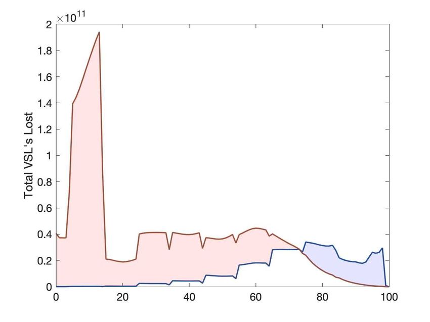
19 crisis, with a specific focus on the intergenerational impacts of lost economic output
and death from disease contagion. It is thus recognized that policymakers may face the
dilemma of enacting policies that reduce short-run deaths but also decrease aggregate
output and health-care efficiency which each have long-run, negative impacts on wel-
fare. Depending on the severity of the recession and how deadly the disease is, under
many policies the damage to long-run welfare may exceed the short-run benefits. Life ex-
pectancy and the consumption value of life for the young are particularly harmed by the
indirect economic factors associated with the current recession. Meanwhile, older adults
are more at risk from dying from the disease. In order for the consumption value of lost
life years associated with COVID-19 to exceed the value of lost years associated with in-
direct factors resulting from a policy-driven recession, the recession needs to be relatively
mild and the number of deaths prevented relatively high. Otherwise, a greater share of
the burden is placed on the shoulders of the young.
    This paper will proceed as follows. Section 2 will present evidence from the literature
arguing why using a welfare measure that depends on health investment is important
to understand the distributional implications of the 2020 COVID-19 crisis. Section 3 pro-
vides a brief overview of the Hall and Jones (2007) model. Section 4 describes the data
used for parameter selection and important outcomes of the estimation. Section 5 simu-
lates various recession and COVID-19 death scenarios to analyze the welfare implications
of the 2020 crisis through the model’s lens. Finally, Section 6 concludes.

2 Background

2.1 Welfare Implications of COVID-19
Many economists have considered the welfare implications of COVID-19. In a model with
no consumer heterogeneity, Eichenbaum, Rebelo, and Trabandt (2020) show that contain-
ing the spread of the contagion may be welfare-improving in spite of the severe recession
such policies cause. By contrast Bethune and Korinek (2020) show that a more nuanced
approach, where infected agents are fully isolated, is socially optimal and yields milder
recessions compared to full shutdowns. Bethune and Korinek (2020) acknowledge that
in the event such a nuanced approach is infeasible aggressive containment is still opti-
mal though very costly. Glover et al. (2020) advocate for a partial, possibly Swedish-style
containment policy. Their approach, like the one in this paper, considers the effects of
shutdowns on different age groups, and they find that elderly consumers benefit far more
than the young from stringent containment policies that vastly reduce economic activity.

                                             3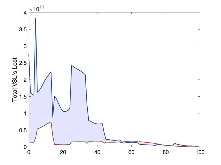
Meanwhile, Correia, Luck, and Verner (2020) attempt to use variation between U.S. cities’
economic shutdown policies during the 1918 Spanish Flu pandemic to argue that short-
term shutdowns to mitigate disease contagion improve long-run growth. Barro, Ursúa,
and Weng (2020) have similar findings. Both results hinge on the fact that working-age
adults were most likely to die from the 1918 Spanish Flu, which is not true in the case of
COVID-19. But, as is shown here, accounting for differences in the age-mortality distri-
bution matters for optimal-mitigation policies.
    The primary contribution of this paper is to consider aggregate welfare implications
in a framework with both endogenous LE’s and VSL’s that are also heterogeneous across
ages and depend on health investment. Results and conclusions presented here conform
more with results in Bethune and Korinek (2020), Glover et al. (2020), and Krueger, Uhlig,
and Xie (2020), suggesting a nuanced response to COVID-19 that does not too drastically
limit commercial activity. Such policies can be aggregate-welfare improving as long as
they reduce overall COVID-19 deaths sufficiently, depending on the various modeling
assumptions.

2.2 The Impact of Recessions and Poverty on Childhood Development
Since this paper argues that the welfare impacts of the COVID-19 recession are dispropor-
tionately shouldered by young people, it is important to understand why policymakers
and economists should care about this by reviewing the literature on recessions, poverty,
and childhood development. Generally speaking, if the 2020 COVID-19 economic reces-
sion leads to increases in poverty and malnourishment amongst children and decreases in
stimulating contact with adults, like educators and mentors, adverse impacts to long-run
welfare should be expected.
    Heckman, Pinto, and Savelyev (2013) establish the long-run, positive impacts of in-
teractive early childhood development programs on the life outcomes of an individual
participant. Heckman (2008) discusses how ability gaps between advantaged and dis-
advantaged children start early in life and can be mitigated by substantial, targeted in-
vestment in early childhood programs. Early environmental factors due to parenting
and familial practices can also lead to better developmental outcomes (Heckman 2008).
But financially-stressed families are less likely to have time for full parental engagement,
which could negatively affect future outcomes for school-aged children of working par-
ents who are out of school due to COVID-19 shutdowns.
    Campbell et al. (2014) find that stimulating early childhood development leads to sig-
nificantly better health and cognitive outcomes during adulthood. In their study, children

                                             4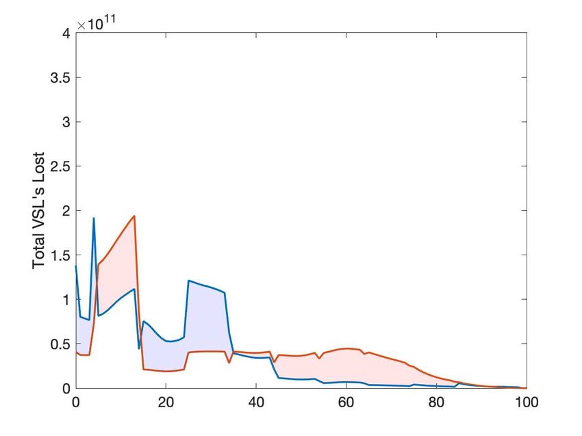
subjected to a treatment where they were engaged in “social stimulation interspersed
with caregiving and supervised play throughout a full 8-hour day for the first 5 years” of
their lives where they were also given “two meals and a snack at the childcare center [and]
were offered primary pediatric care” had significantly lower risk for non-communicable
diseases in their mid-30s (Campbell et al. 2014). Hoddinott et al. (2011) provide strong
evidence that sustained investments in early-life nutrition and childhood development
lead to welfare improvements over the life cycle and thus the long run. If the current
shutdown not only leads to less stimulating social contact but also limits the ability of
impoverished children to benefit from free school breakfast and lunch programs, school
closures will have adverse impacts that affect social, intellectual, and physical develop-
ment.
    The evidence on child health outcomes resulting from economic contractions versus
expansions is mixed. Ferreira and Schady (2009) review empirical evidence finding that
in rich countries, like the U.S., recessions may not have an adverse impact on the health
and human capital development of children. Indeed, they find that child health and ed-
ucational outcomes appear counter-cyclical. The counter-cyclical nature of educational
outcomes for children may be due to the outsize, positive effect of the Great Depression
on high school graduation rates (Goldin 1999; Black and Sokoloff 2006). Recent microe-
conomic evidence in the U.S. also suggests that infant mortality may be counter-cyclical
(Chay and Greenstone 2003; Dehejia and Lleras-Muney 2004; Ferreira and Schady 2009).
But, while infant mortality may be countercyclical, there is evidence that out-of-pocket
spending on childhood health care services is pro-cyclical, especially for children with
a high baseline level of medical care (Karaca-Mandic, Choi Yoo, and Sommers 2013).
Such children often have special needs and are more sensitive to pullbacks in medical
care spending. Further evidence from developing countries suggests that on the whole,
children’s health outcomes are made worse by recession, with potential long-run con-
sequences resulting from malnutrition and stunted growth (Jensen 2000; Stillman and
Thomas 2004; Paxson and Schady 2005; Alderman, Hoddinott, and Kinsey 2006; Ferreira
and Schady 2009).
    Other microeconomic studies focussing on parents’ labor market outcomes suggest
that economic downturns likely harm childhood development more than they open up
opportunities for developmental improvement. Kalil (2013) reviews the preponderance
of evidence as to how parental job loss and income instability affect childhood develop-
ment, concluding that the Great Recession likely adversely affected children’s long-run
economic outcomes. For example, parental job loss, especially in families with lower so-
cioeconomic status, is associated both with negative effects on educational outcomes and

                                            5
behavioral and emotional health problems for children during their teenage years (Ore-
opoulos, Page, and Stevens 2008; Ananat et al. 2011; Kalil 2013). Further, the adverse
impacts on emotional and psychological health of children experiencing parental job loss
appear to persist for at least five years (Kind and Haisken-DeNew 2012). Many studies
suggest that mere perceptions of parents’ job insecurity are enough to cause stress that
leads to poor educational outcomes and behavioral problems (Barling, Dupre, and Hep-
burn 1998; Barling, Zacharatos, and Hepburn 1999; Conger and Donnellan 2007; Ananat
et al. 2011; Schneider, Waldfogel, and Brooks-Gunn 2015). This is because fear and anx-
iety can tax cognitive skills, adversely affecting behavioral health (Leininger and Kalil
2012; Shah, Mullainathan, and Shafir 2012). Given the high unemployment numbers seen
during the 2020 economic crisis, we should expect that familial stresses induced by job
insecurities are at play, possibly affecting children’s health outcomes.
    Poverty in general, whether wrought from aggregate shocks or just bad luck, induces
stress and results in adverse child-development outcomes (Boyer and Halbrook 2011).
Childhood stress can manifest itself as poor physical health outcomes during teenage
years (Evans and Schamberg 2009). It can also stunt brain development and limit the
ability of the individual to engage in complicated cognitive functions, like deep critical
thinking, in the future (Sapolsky 2004). Disparities in academic outcomes in early school-
ing years brought on by a lack of initial human capital development may be magnified as
children progress through school (Cunha et al. 2006). In conclusion, childhood poverty is
associated with poor outcomes during adulthood, including a higher propensity for crim-
inal behavior, mental illness, and general health disparities (Evans and Kim 2007; Evans
and Schamberg 2009; Nikulina, Widom, and Czaja 2011; Kim et al. 2013).
    Thinking about the dynamic, long-run impacts of economic shocks to individuals
across the age distribution, especially with respect to health outcomes, will help build
inference as to which policies can dampen and mitigate recessions’ adverse effects on
children. In light of evidence that directly links the health and viability of adults to their
early childhood education (Campbell et al. 2014), policies that reduce negative impacts of
recessions on childhood cognition should be considered.

2.3 Measuring the Value of Statistical Lives
In this paper, the primary exercise is to analyze a dynamic model that generates en-
dogenous measures of LE and VSL as a result of the consumption and health invest-
ment choices of age-heterogeneous agents. While the model will generate a measure of
VSL that relies on how marginal changes to health investment improve age-specific, non-

                                              6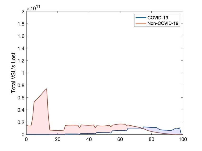
accidental mortality rates, in the literature such a measure of VSL is rather uncommon.
To the best knowledge of this author, the only other paper that attempts to estimate VSL’s
using both mortality rates and age-specific health spending is Hall and Jones (2007), from
which the model here is borrowed directly with a few slight modifications.
    In the empirical literature, VSL’s are typically estimated using labor market outcomes.
Specifically, one can regress the between-industry wage premium on differentials in industry-
specific accidental mortality rates, while controlling for skills and human capital. In the
VSL literature, this is known as the “revealed preference” approach. Other approaches,
known as “stated preference” approaches, explicitly ask individuals how much they would
be willing to accept in exchange for increased risk of death. Viscusi and Aldy (2003) and
Kniesner and Viscusi (2019) provide a review of both of these strands of the VSL litera-
ture, suggesting that for working-age men, VSL’s are $10 million in 2018 dollars. That
is consumption value of an average working-age male’s life is around $10 million. But,
some authors have criticized estimates from labor market measures as quantitatively frag-
ile, since skills and human capital are difficult to observe (Siebert and Wei 1994; Leigh
1995; Miller 2000; Hintermann, Alberini, and Markandya 2010). Nordhaus (2002) criti-
cizes measures of VSL from the labor market literature because they fail to account for
possible dynamic changes to both future risk and future income, as such estimates only
reflect a current risk to current income tradeoff. This is problematic considering that mor-
tality premia have risen along with the health services share of consumption (Nordhaus
2002, 2005). Such a criticism thus provides impetus for alternative models which generate
VSL’s using health spending and mortality outcomes, as is done in this paper.
    Further, using labor market outcomes to quantify VSL’s can be limiting since not all
age groups actually work. Specifically, VSL’s for children and elderly retirees are ignored
in such studies. This may be problematic since Aldy and Viscusi (2008) find significant
correlations between VSL and age for workers in different age groups. They conclude
that VSL follows an inverted-U-shaped profile, where younger workers in their late teens
and early twenties and older workers nearing retirement have similar VSL’s of around $5
million in 2018 dollars, while prime-age workers have VSL’s over $13 million. But how
can we measure the VSL for, say, a 10-year old when using only labor market outcomes?
    To estimate youth VSL’s, some studies rely on parents’ willingness to pay (WTP) to re-
duce childhood risks of death or trauma. Byl (2013) uses evidence from the infant car-seat
market to show that children’s lives are valued at a premium to adults’. This premium
is almost double and could be as high as $17 million in inflation-adjusted 2018 dollars.
Jenkins, Owens, and Wiggins (2001), using the market for bicycle helmets, estimate sep-
arate VSL’s for children and adults, finding the opposite of Byl (2013): adults’ lives are

                                            7
typically more valuable. Other authors have used stated-preference surveys to ask adults
how much they would pay to reduce the risk by half of a child being killed by a parent
or caregiver (Corso, Fang, and Mercy 2011; Peterson, Florence, and Klevens 2018). Such
surveys conclude that the level of VSL for children is around $17 million in 2018 dollars.
Hammitt and Haninger (2010) also find significantly higher VSL’s for children using a
stated-preference survey involving willingness to pay to reduce risk from fatal diseases
and traumas — around $16 million for children versus $7-12 million for their parents.
    While there seems to be a consensus in the literature as to the range of plausible VSL’s
for adults, there is debate as to the shape of the life-cycle VSL profile when younger age
groups are included. The findings presented in this paper, as well as those in Hall and
Jones (2007), suggest that VSL’s are likely declining, almost monotonically, in age. The
results here thus confirm many of the aforementioned WTP studies, while contrasting
with the age-profile VSL estimates of Aldy and Viscusi (2008).
    This paper takes the health production approach to measuring age-specific VSL’s. It
is thus assumed that increases in health investment lead to decreases in non-accidental
mortality and thus increases in life expectancy. VSL’s are then identified parametrically
by the marginal cost, in consumption units, of decreasing the non-accidental mortality
rate. The approach presented here thus relies on a revealed preference argument: the
investments made in children’s health care by society as a whole reflect how much value
society places on children’s lives. Indeed, as will be shown, children enjoy a large VSL
premium over their parents when using health investment data.

3 Model
In modeling how a sudden and unexpected disease contagion simultaneously affects both
economic and health outcomes, we turn to the centralized endowment economy in Hall
and Jones (2007). In their dynamic model, health investment by consumers positively
affects health status through a health production function that is both age- and time-
dependent. Increases in health status lead to declines in mortality risk, raising the proba-
bility the age-a consumer in period t will live to be an age-a + 1 consumer in period t + 1.
Consumers thus face a tradeoff in choosing consumption c at , which yields flow utility to-
day, versus health investment h at , which increases the probability of future survival and
thus the value of future consumption flow utilities. In this manner, health status and thus
survival probabilities are endogenous.
    The model here departs from Hall and Jones (2007) by assuming the period-length is
one year instead of five. Consumers live up to age 100, so in any given period there are

                                             8
101 cohorts of consumers alive, counting newborns. Each age-a cohort in period t is char-
acterized by a representative agent, so that there is no heterogeneity within age groups,
only across age groups and over time. In any given period, there are Nat consumers of age
a alive. Every consumer is assumed to contribute the same amount yt to net resources,
so that yt can be thought of as income per-capita. From this assumption, all variation in
contributions to aggregate welfare across age groups and over time is strictly dependent
on variation of per-capita health investments by age.
Using endogenous health investment, the model generates measures of VSL by age
from the marginal cost of health production. This permits analysis as to how different co-
horts are disparately impacted by both aggregate output shocks affecting yt and shocks to
health care technology directly impacting health status. Each of these channels will affect
welfare measures which rely on VSL’s. First, health investment will vary as net resources
change, affecting the marginal cost of health production and thus mortality rates. Sec-
ond, changes in the productivity of health services will directly affect the marginal cost of
health production for any given level of health investment. But, this will also induce con-
sumers to adjust their health investments as long as mortality risk is not perfectly inelastic
with respect to health investment.
Denote health status as x at , which is a function of health care consumption h at , an ag-
gregate health sector productivity component zt , and an idiosyncratic, age-specific com-
ponent w at , so that x at = f a (h at ; zt , w at ), where f a is increasing in all arguments. h at can
also be thought of as health investment, since its purchase level has dynamic, long-run
implications for survival. w at accounts for factors orthogonal to health technology ad-
vancement, like un-modeled decisions related to education or habits like smoking and
drug use. Hall and Jones (2007) assume zt and h at account for some known fraction µ of
the decline in U.S. mortality rates over the last half century, while w at accounts for the re-
mainder. This leads to an identification issue which is addressed in Section 4.1, re-visiting
some fundamental findings from the health outcomes literature.
Health status, x at , is the inverse of the age-a, period-t mortality rate, m at = 1/ x at .
Survival rates are thus 1 − m at = 1 − 1/ x at . Total mortality is the sum of accidental m acc at
and non-accidental mnon at mortality. Health care investment decisions h at are assumed to
only affect non-accidental mortality, so that health status can be written
1 1
x at = f a (h at ; zt , w at ) = = acc (1)
m acc
at
non
+ m at m at + 1/ xeat
xeat (h at ) = A a ( zt h at w at )θa (2)
In addition to choosing h at , consumers also choose other consumption c at . They receive
9c1−γ
flow utility from c at according to the iso-elastic function u(c at ) = 1at−γ .2
Each consumer receives exogenous endowment income yt which evolves according to
some known process. All risk is thus idiosyncratic and endogenous, acting through the
survival function. Finally, each period assume consumers have base utility b at , which will
be calibrated to ensure that the value of life is zero upon death. As Hall and Jones (2004)
discuss in their working paper, b at will usually be positive since calibrated choices of γ
are > 1, ensuring that u(c at ) < 0. There is no savings mechanism and labor is assumed
to be supplied inelastically.
Under these conditions and assuming equal Pareto weights for all agents alive in pe-
riod t, the social-welfare maximizing allocations satisfy
∞
Vt ( Nt ) = max
{h at ,c at } a
∑ Nat b at + u(c at ) + βVt+1 ( Nt+1 ) (3)
a=0
∞
subject to ∑ Nat ( yt − cat − hat ) = 0 (4)
a=0
1
Na+1,t+1 = 1− Nat (5)
x at
x at = f a (h at ; zt , w at ) (6)
yt+1 = e g yt yt (7)
where Nt is a vector with components N1t , N2t , . . . , Nat , . . . describing the population dis-
tribution in t, and β ∈ (0, 1) describes a consumer’s time preferences.3
Optimal allocations of {h at , c at } a are subject to the equilibrium condition
β v a+1,t+1 x2at
= ∀ a, t (8)
u f ′ (h )
| {zc } | {zat }
Marginal Benefit of Saving a Life Marginal Cost of Saving a Life
∂V
v a+1,t+1 is the standard envelope condition, ∂N t+1 , which captures how the total future
a+1,t+1
value of social welfare changes in response to variation in the population level of agents
surviving from age a in t to become age a + 1 in t + 1. Under the parameterization of
2 Hall and Jones (2007) consider both a flow utility function that only features other consumption and one
where consumers benefit from health status. This so-called “quality of life” utility component is omitted
here, without loss of generality. Indeed, Hall and Jones (2007) show that regardless of whether the quality
of life component is included, VSL estimates are hardly affected.
3 The planner’s optimization problem is the same as that in the working paper Hall and Jones (2004),
where base utilities are allowed to be both age- and time-dependent. This specification is preferred to that
in the published version of the paper, so that b at can be directly calibrated to match VSL’s estimated from
health investment technology.
10health technology in (2), the right hand side of (8) is h at xeat (h at )/θ a , which is a measure of
VSL. In practice, the age- and time-varying utility intercepts b at , can be backed out of (8) to
ensure that the empirical estimates of VSL’s, using the marginal cost of health production
on the right, exactly equal the marginal benefit attributable to household preferences.
That is, given data on health outcomes, income, consumption, b at can be calibrated to
force (8) to hold.
4 Parameter Selection
Updating both versions of Hall and Jones (2004, 2007), the health production parameters
are selected using a regression of survival probabilities on health spending that accounts
for possible trends in age-specific residuals, w at . The estimation of xeat (h at ) is described in
detail in Section 4.1, where several assumptions on the fraction of trend decline in mor-
tality associated with technological change, which is denoted by µ , are considered. With
health production parameters, productivities, and residuals in hand, age-specific, period-
t VSL’s can be computed using the marginal cost approach: VSL at = h at xeat (h at )/θ a . Hav-
ing VSL’s, base utilities b at , can be backed out of the equilibrium condition (8) following a
procedure described briefly in Section 4.2. Finally, in Section 4.3, given the health produc-
tion parameters, productivities, and base utilities, the model is solved backwards from
2018 to 1959 by simulating equilibrium choices of c at and h at for yt computed from NIPA.
4.1 Estimating Health Production Parameters
Aggregate NIPA data from 1959-2018 and age-specific health spending data from Meara,
White, and Cutler (2004) are used to estimate A a and θ a for each a. Aggregate health
spending is the sum of personal consumption expenditure (PCE) on health care and gov-
ernment spending on health care. All other non-health-care consumption is the sum of
other PCE spending and non-health-related government spending. To compute these
data points, we can turn to NIPA’s PCE Tables 2.5.3, 2.5.4, and 2.5.5, and the government
outlay Tables 3.15.3, 3.15.4, and 3.15.5. Dealing with unit-uniformity issues arising from
combining chain-weighted price and quantity indices, the procedures in Whelan (2002)
are used to construct new indices for the combined aggregate series using both PCE and
government spending. Using the aggregated health spending data, age-dependent health
spending distributions are constructed by utilizing the weights for five-year age groups
described in Meara, White, and Cutler (2004) and interpolating both within periods across
age groups and over time to arrive at annual distributions of health spending from 1959
11to 2018 for consumers of ages 0 to 100. A cubic polynomial is used for interpolation over
the time dimension. Where extrapolation is required, assume the health spending distri-
bution across ages is stationary after the last year of observations in the sample.4 Within a
period, a simple replication scheme is followed: since health spending data is only avail-
able for individual averages over ten-year age groups, the same health spending level is
assigned to all individuals within an age group. For age-specific mortality data, several
sources for both accidental and non-accidental mortality rates are used — for years 1950
to 2003, the National Center for Health Statistics report, Health, United States, 2003, and
for years 2004 to 2017, the National Vital Statistics Reports, Volume 68, Number 9, Deaths:
Final Data for 2017, updated on June 24, 2019. Finally, life-expectancy data, which are not
directly used in the estimation but matched independent of parameter selection, are taken
from Table 4 of the 2017 National Vital Statistics Reports.
With health investment and mortality data, (2) is estimated separately for each age-a
consumer unit using a two-step regression procedure where the trend in w at is assumed
orthogonal to health outcomes xeat whenever it is also assumed that some fraction µ of
mortality trend decline is attributable to non-technological factors. Note that when µ = 1
all trend decline in mortality is assumed to be attributed to technological change acting
through either zt or yt via h at . For more details on this identification argument see the
discussion in Hall and Jones (2007).
Here, two separate assumptions on µ are considered and the orthogonality restriction
for the trend in w at is assessed using a C-test on the difference in two Sargan/Hansen
statistics described in detail in Hayashi (2000). In all cases the growth rate in zt is assumed
to be identical to growth in yt , i.e. g z = g y . This assumption is affirmed by empirical work
in Horenstein and Santos (2019) who find little evidence to suggest productivity growth
in the health sector substantially differs from GDP growth. In the first exercise, it is as-
sumed that µ = 1, so that all decline in mortality is due to technical advancement. In the
µ = 1 case, the orthogonality of trend in w at is irrelevant. Alternatively, examining the
case where µ = 2/3 as in Hall and Jones (2007) allows for the orthogonality restriction on
trend growth in w at to be tested. The C-test fails to reject such a restriction, so gwa t is used
as an instrumental variable (IV). This empirical result jibes with the original findings in
Hall and Jones (2007) and other studies which suggest that factors not related to health
spending have played an important role in mortality rate declines (Fogel 2004; Grossman
2005; Cutler, Deaton, and Lleras-Muney 2006). The preferred health production specifica-
4 This extrapolation assumption was tested where the extrapolated data using the Meara, White, and
Cutler (2004) age-specific health spending estimates were compared against data from the Centers for Medi-
care & Medicaid Services (CMS 2019). Differences between the age-distributions of health investment are
insignificant. The results of this test are available upon request.
12tion is thus the 2SLS estimation where µ = 2/3 and gwa t is used as an IV.
(a) Health Production Intercept (b) Elasticity w.r.t. Health Investment
Figure 1: Here, plots of the estimates for ln A a and θ a are presented. The cases where
µ = 1 and µ = 2/3 with no trend instrument track each other in terms of the declining
profile by age. The IV versus non-IV regressions yield similar estimates except for the
15-25 age group. All estimates of θ a are significant at the 1% level.
Figure 1 presents estimates for the time-independent health production parameters,
where age indexes the horizontal axes. The stair-step feature of the estimates reflects the
interpolation scheme assigning the same health and survival rates to everyone in ten-year
age groups. In the µ = 2/3 case, the introduction of the linear-trend IV only significantly
affects inference as to the elasticity of health outcomes θ a for 15-25 year olds, which can
be seen by looking at the differences in the gold versus red lines in Figure 1b.
Focussing on θ a , notice that this elasticity appears to consistently decline in age, with
the exception of the jump for teens and young adults. Its negative, −θ a , is the elasticity
of the preventable mortality rate with respect to health spending. It thus represents the
percent change of a percentage-point decline in mortality with respect to health spending.
To fix intuition as to why θ a mostly declines with age, consider the non-accidental mor-
tality rates of a 30-year old and a 70-year old. Currently, a 30-year old has a probability
of dying before he reaches age 31 of approximately 0.0006, or 0.06%, while a 70-year old
has a probability of dying before reaching age 71 of 0.0175 or 1.75%. Estimates of θ30 and
θ70 for the µ = 2/3 case with no IV are 0.6540 and 0.4012 respectively. A 1% increase in
health spending by a 30-year old thus leads to a 0.65% reduction in the mortality rate, so
that the new mortality percentage is 0.02%, amounting to an absolute reduction of 0.04%.
Meanwhile, for a 70-year old, a 1% increase in health spending leads to mortality declin-
ing from 1.75% to 1.05%, or 0.7% in absolute terms. Thus, despite the fact that θ70 < θ30 ,
13a 1% increase in health spending for a 70-year old actually has a greater impact on overall
mortality-rate decline because the 70-year old is starting at a base rate that is substantially
lower than that of the 30-year old.
(a) Productivity Levels, 2018 = 1 (b) Productivity Growth Rates
Figure 2: These plots illustrate both the evolution of age-weighted health productivities
(a) and the age-specific growth rates (b). In panel (a) estimates are projected out to 2100
to illustrate the differential rates at which returns to health care investment evolve for
different age groups. In panel (b), estimated health productivity growth rates from 1959
to 2018 show that younger and older adults benefitted the most from residual returns to
health care efficiency zt and other age-specific indirect factors w at over the latter half of
the twentieth century.
Figure 2 shows the age-weighted productivity levels and growth rates over time under
the assumption µ = 2/3. Age-weighted growth is (1/µ − 1) ( gha + g z ) + g z . Both older
and younger age groups experience faster health productivity growth than working-age
adults. The measure of productivity presented here accounts both for changes in the total
factor productivity of health services zt and changes to the idiosyncratic, age-specific com-
ponent w at , which captures other exogenous factors, unrelated to health services produc-
tivity. These include everything from improvements to public-school lunch and nutrition
programs for children to heightened on-the-job safety standards for adults, as well as the
effects of changes to pollution, urban density, and other environmental forces. w at , espe-
cially for young agents, will capture the aforementioned residual, non-health-technology
impacts of the 2020 recession, such as factors resulting from school closures adversely
affecting young agents’ health outcomes. Multiplied together, zt w at then captures the de-
gree to which returns to health productivity zt are either enhanced or dampened by these
other age-dependent factors.
144.2 Estimating Base Utilities, b at
To compute b at , an estimate of VSL at is needed so that the health production function
TFP and elasticity estimates can reconcile both c at and h at in a full decision-theoretic equi-
librium environment. The right-hand side of (8) is a measure of VSL at , which can be
computed using only health data and fitted health production parameters. Thus, after
fitting the health production function, with an estimate for VSL at in hand and assuming
that v101,t = 0 for all t, β v a+1,t+1 can be backed out and the model’s full Lagrangian
expression can be used to compute
v at = b at + u(ct ) + β v a+1,t+1 + uc ( yt − ct − h at ) (9)
where uc is the marginal utility of consumption, and output per-capita, consumption per-
capita, and health investment are data. Note that, given the problem here is that of a
planner efficiently allocating resources, it is without loss of generality that ct = c at since,
by the Second Welfare Theorem, there exist implicit transfers reconciling this efficient
allocation for a de-centralized environment.5 With b at in hand, it remains only to vary γ
and β to solve for equilibrium values of ct and h at generated by the full decision-theoretic
model.
4.3 Equilibrium VSL’s and Life Expectancy
Given γ , β is selected to match consumption growth gc from a classical Euler equation,
so that β = (1 + gc )γ /1.04, where 1.04 is assumed to be the gross interest rate and
gc = 0.0168 — average per-capita consumption growth from 1959-2018. Given b at and
the health production parameters, the model is solved using several values of γ selected
over the interval (1, 2]. γ = 1.25 best matches the life expectancy of newborns and the
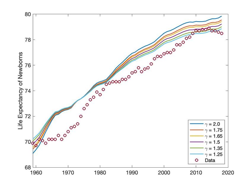
aggregate share of health spending in 2018. Figure 3 presents model-generated equilib-
rium LE’s of newborns under different values of γ along with LE estimates from data.
The model’s equilibrium appears to adequately capture the increasing profile over time.
γ = 1.25 is used for the upcoming simulations because the equilibrium time series un-
der this assumption appears to provide the closest match to LE’s from the data in 2018.
Further, lower values of γ are associated with greater leveling-off in long run LE growth,
which is also apparent in the data, especially in the decade after the Great Recession.
In equilibrium, the model generates estimates for working-age adults’ VSL’s in line
with VSL estimates from labor market outcomes. Table 1 presents these estimates for the
5 Hall and Jones (2007) also recognize this fact, as evidenced by their calibration scheme.
15Figure 3: This plot presents the life expectancy of newborns from the simulated model
equilibria under different values of γ alongside life-expectancy data taken from the Na-
tional Vital Statistics Reports. In all separate simulations where γ is varied, it is assumed
that µ = 2/3 and health production function estimates from the 2SLS model are used. The
preferred specification has γ = 1.25, which most closely matches life expectancy data in
2018, the last year in the present data sample.
preferred specification where µ = 2/3, γ = 1.25, and health production parameters are
taken from the 2SLS regression with a trend IV. Both cumulative VSL’s and VSL’s divided
by age-specific LE, where the latter is a measure of the value of life per year of life saved,
are presented. 2018 VSL estimates for 30, 40, and 50 year olds in the baseline model range
from $4 to $9 million. Estimates using Mincer-style regressions on wages and industry-
specific mortality risk, which are thoroughly reviewed in Kniesner and Viscusi (2019),
suggest values within this range. Meanwhile, VSL estimates for children are notably
higher and exceed the ranges of estimates from microeconomic studies looking at parents’
WTP for child-safety products and reviewed in this paper in Section 2.3.
Notice that, not only do children have higher VSL’s measuring the expected consump-
tion value of their remaining life years (top half of table), but some, particularly 10-year-
olds, also have higher VSL’s per life-year remaining (VSL/LE in the bottom half of the
table). Now consider the fact that there are far more children between the age of say
5 and 15 than elderly people between the age of say 75 and 85. Suppose an arbitrary
16Table 1: Equilibrium VSL’s, γ = 1.25, µ = 2/3 with IV
Value of Life in Thousands of 2018$
Age 1960 1970 1980 1990 2000 2010 2018
0 2010.966 3330.654 4763.997 6525.515 7996.263 8935.804 9552.773
10 5854.994 8033.472 11068.602 16009.304 21853.497 29520.890 34287.264
20 1889.003 2223.565 2679.445 3655.983 4916.239 6113.957 6841.157
30 2672.409 3614.118 4547.095 6298.397 8388.125 8932.166 8281.171
40 1534.607 2344.928 3161.870 4411.828 5495.411 6220.439 6202.894
50 793.792 1347.851 1890.560 2717.719 3485.834 4009.968 4404.305
60 506.081 914.671 1332.577 1944.938 2556.526 3049.265 3482.870
70 439.982 799.947 1166.095 1714.775 2247.303 2666.708 3100.446
80 452.276 799.654 1124.982 1622.251 2103.413 2426.037 2763.816
90 412.520 716.010 979.319 1383.096 1769.241 2017.137 2194.594
Value of Life per Year of Life Remaining in Thousands of 2018$
Age 1960 1970 1980 1990 2000 2010 2018
0 28.958 46.452 64.840 86.651 104.302 115.317 122.684
10 97.375 129.009 173.109 243.731 326.261 435.649 503.326
20 37.353 42.167 49.285 65.235 85.832 105.394 117.244
30 64.834 83.254 101.022 135.150 175.666 184.334 169.622
40 47.771 68.404 88.287 118.234 143.133 159.137 156.979
50 33.427 52.384 69.720 95.470 118.329 133.165 144.156
60 30.552 50.277 68.955 95.161 120.207 139.696 156.764
70 41.031 67.271 91.862 127.021 159.315 183.833 209.797
80 70.835 113.389 150.135 204.224 253.941 285.457 321.687
90 109.947 175.853 229.368 309.328 382.910 428.040 465.715
drop in economic activity causes all VSL/LE’s to decline by a fixed percentage across the
board. The per-capita hit to children will be higher than to others since they have such
high starting VSL/LE baselines. Further, the total impact on each age group will be higher
for younger cohorts than older ones because there are more youths than senior citizens.
In the context of a disease whose mortality rates are disproportionately skewed toward
older people, policies designed to curb the spread of disease in order to preserve lives
while simultaneously causing an economic recession thus amount to a transfer of welfare
from young to old. This phenomenon is explored in more detail in the simulations in
Section 5.
175 The Welfare Impacts of Disease Contagion
Aggregate shocks will affect income and possibly health investment and thus health out-
comes. Aggregate shocks coupled with a global pandemic will also affect the efficiency
of health investment when it comes to generating health outcomes. This is because a
pandemic strains health care systems due to large numbers of people with acute illnesses
requiring immediate care. Indeed, this potential capacity problem was the main reason
why many localities quickly enacted measures to mitigate the spread of COVID-19 in the
early weeks of the contagion. For April and May, many U.S. localities allowed only essen-
tial medical procedures to occur, so that consumers were forced to put off preventative
care and elective surgeries despite still paying insurance premiums which would cover
such procedures. Money spent for health care during this time was thus spent less ef-
ficiently as multiple weeks and months passed with preventative and elective care put
on hold. Thus, while those policies were implemented to seemingly maintain capacity
and efficiency in the health care system, health outcomes beyond those directly related to
the COVID-19 pandemic may still have been adversely affected. While health efficiency
shocks are represented by a drop in zt , the 2020 recession has also likely brought on resid-
ual shocks to w at . Aside from the adverse residual effects on childhood development
which have been discussed, gym closures may restrict adults’ exercise regimens, and
families confined to close-quarters for months on end may be more likely to engage-in
and/or experience abusive behavior, amongst other possible outcomes.
In terms of the model here, the U.S. economy therefore experienced two simultaneous
aggregate shocks to welfare, independent of health outcomes that directly result from
the COVID-19 pandemic: 1) a reduction in yt affecting health investment choices; 2) a
reduction in zt w at affecting the efficiency of those same choices. COVID-19 overwhelm-
ingly affects individuals with compromised immune systems who are older. The degree
to which COVID-19 causes premature deaths for consumers of different ages combined
with the degree to which consumers of different ages are differentially affected by both
shocks to yt and zt w at will determine how the present crisis adversely impacts individuals
across the age distribution.
In this section, equilibrium outcomes under several scenarios are considered in or-
der to account for uncertainty around the magnitude of the economic shocks, as well
as mortality directly caused by the COVID-19 contagion. Specifically, life expectancies,
and VSL’s for people of all ages change in response to income and health productivity
shocks. Several shock scenarios are simulated relative to a baseline where yt and zt w at
18continue to grow at their pre-COVID rates.6 The simulations can be divided into two
camps: 1) those where both yt and zt w at are shocked, while accounting for differential
COVID-19 mortality risk across the age-distribution; 2) the same as the first simulation,
except replacing COVID-19 mortality risk with age-specific estimates for the 1918 Span-
ish Flu. The latter counterfactual exercise is undertaken in order to assess the importance
of the disease contagion’s age-mortality distribution on both aggregate and distributional
welfare outcomes.
In each broad camp, there are six separate scenarios for income and health productiv-
ity shocks.7 The first income shock scenario builds on the Congressional Budget Office’s
(CBO) May 2020 projections of output loss due to the policy-driven recession (CBO 2020).
The CBO estimates a −5.6% annual growth rate for 2020 followed by 4.2% for 2021. An
L-shaped recession is considered in scenario two, where output falls −5.6% in the first
year and recovers thereafter only at the post-Great Recession rate of 0.98%. Next, a quasi-
V-shaped recession is considered where output falls by 5.6% in 2020 and rises by 5.6%
in 2021. Finally, these exercises are repeated after adjusting the magnitude of the initial
shock to −10%.
The six scenarios for health productivity shocks directly correspond to the income
shock processes. Assume that health productivity shocks and recovery rates are propor-
tional to those of yt . For example, suppose that output continued to grow at the post-
Great Recession rate, and call the level of 2020 per-capita output associated with this
growth y2020 . Then, a −5.6% year-on-year shock to 2019 output leads to a reduction in
2020 output relative to y2020 of −0.056 − 0.0098 = −0.0658. Now, note that baseline
g z + gwa can be computed under the assumption that µ = 2/3 and a further assumption
that zt grows at the same rate as yt . In every different shock and recovery scenario and for
each age-a agent in each subsequent period after the shock, the log of age-specific produc-
tivities zt w at can be rescaled by the proportional growth factor (in this example, −0.0658)
6 Specifically,
assume that had COVID-19 not occurred, yt would continue to grow at its post-Great Re-
cession annual rate of 0.0098 and zt w at would evolve along its constant, age-specific growth path presented
in Figure 2a.
7 It should be noted that all shocks are modeled in the “MIT” sense. That is, they occur suddenly and
without expectation. Indeed, consumers and thus the social planner are not thought to have any idea that
such a shock were to ever be possible, thus failing to plan for it. The model is first solved for equilibrium
outcomes using output growth and population projections out to year 2100, assuming that no adverse shock
pertaining to a contagion has occurred in 2020. Then, having equilibrium consumption and health invest-
ment decisions in hand, per-capita income yt and health productivities suddenly decline, corresponding to
the recession and recovery characteristics described above. In this formulation, with a period length of one
year, 2019 is the last period prior to the shock affecting output in 2020. Recovery begins in 2021 in every
scenario, and the simulations are conducted by solving the model backwards from 2100 where per-capita
growth after 2021 is projected out at the model-implied post-Great Recession (after 2009) annual average of
0.98%.
19relative to the baseline. Having now shocked both yt and zt w at , equilibrium outcomes
can be computed.
5.1 Joint Income and Health Investment Productivity Shocks Account-
ing for COVID-19 Mortality Risk
COVID-19 itself, being an acute event, has little impact on the LE of the young, because
mortality rates from the disease are skewed toward older people. Rather, LE is impacted
through channels residual to the COVID-19 crisis, such as the drop in income and health
investment due to the economic fallout. This section considers the distributional impli-
cations of the economic shutdown while accounting for health productivity shocks and
shocks to mortality directly resulting from the crisis. Indeed, shutting down the economy
amounts to a transfer of welfare from the young to the old. Depending on the ultimate
severity of the crisis, the value of life years lost attributable directly to people dying from
the COVID-19 disease may be exceeded by the value of life years lost due to the non-
COVID-19 residual economic impacts.
Note that the analysis here takes no stand on whether shutting down the economy
to reduce COVID-19 deaths is somehow optimal. Rather, the focus here is on the trade-
off between the value of short-run lives saved and long-run lives lost when VSL’s are
age-dependent and health investment heterogeneity ensures that consumers of different
ages are differentially-affected by economic shocks. Unlike work in Bethune and Korinek
(2020), Eichenbaum, Rebelo, and Trabandt (2020), Glover et al. (2020), and Krueger, Uh-
lig, and Xie (2020) the model here contains no mechanism endogenously linking output
loss to reductions in total disease-related deaths. Rather, income and total disease deaths
are exogenous. Since there is so much uncertainty surrounding how the economic cri-
sis and, ultimately, the disease contagion will play out, this assumption allows for direct
comparison of outcomes under differing degrees of simultaneous economic and disease
contagion. Specifically, the exercises here involve simulating VSL’s and LE’s under dif-
ferent combinations of output shocks and total disease deaths to understand how welfare
loss is distributed between generations. The goal of such an exercise is to understand
how people of different ages are affected by these simultaneous occurrences.
As of July 9, 2020, over 126,000 people in the U.S. had died of COVID-19 (JHUM 2020).
According to the Centers for Disease Control and Prevention (CDC), over 59% of deaths
were individuals 75 years of age or older, and over 80% of deaths were individuals 65
years of age or older (CDC 2020c). Letting mcovid a,2020 denote the age-specific mortality rate
from COVID-19 taken from the CDC’s provisional COVID-19 death counts, the mortality
20distribution associated with COVID-19 can be computed. Specifically, since the CDC
currently reports the total number of deaths by age for each week of the pandemic back
to February 1, 2020, there exists data for the conditional age-distribution of all current
COVID-19 mortalities. Figure 4 presents the age-distribution of COVID-19 deaths where
each line corresponds to a different week of the pandemic. Notice that the age-specific
death distribution has been stable over time and skews older.
Figure 4: Age bins are on the horizontal axis. The different lines represent the distribution
of COVID-19 deaths by age conditional on getting the disease for different weeks of the
pandemic. The sample begins the week starting Sunday, March 8, 2020, and concludes
with the week ending Saturday, June 27, 2020 (CDC 2020c). The conditional age-specific
death distribution appears stationary over time.
While Figure 4 shows the probability of dying from COVID-19 conditional on getting
the disease, the age-specific marginal probability of dying from the disease, mcovid
a,2020 , also
depends on the total number of deaths and the population levels of different age groups.
Using the COVID-19 forecasting models presented at the CDC’s main forecasting hub for
4-weeks out,8 mcovid
a,2020 is computed for seven separate scenarios of total disease deaths: 1)
average 4-week deaths across all models cited by the CDC of 145,224 which is closest to
4-week projections from the Notre Dame-FRED COVID-19 forecasts (ND 2020); 2) maxi-
mal 4-week ahead deaths of 180,226 predicted by Columbia University’s Shaman Group
(CU 2020); 3) 250,000 deaths; 4) 500,000 deaths; 5) 750,000 deaths; 6) 1,000,000 deaths; 7)
1,500,000 deaths; 8) 2,000,000 deaths. Scenarios (3) through (8) account for how the crisis
8 See CDC (2020b) for a full list and description of the models the CDC uses for COVID-19 case and death
forecasting and CDC (2020a) for the actual forecasting data.
21You can also read