Should Germany Have Built a New Wall? Macroeconomic Lessons from the 2015-18 Refugee Wave
←
→
Page content transcription
If your browser does not render page correctly, please read the page content below
Should Germany Have Built a New Wall?
Macroeconomic Lessons from the 2015-18 Refugee Wave∗
          Christopher Busch†               Dirk Krueger‡             Alexander Ludwig§
                            Irina Popova¶               Zainab Iftikhark

                                               Abstract

          We evaluate the macroeconomic and distributional effects of the recent wave of
      refugee immigration into Germany, increasing immigration from its long-run average
      of 200,000 per year to about one million both in 2015 and 2016. To do this we develop
      a quantitative overlapping generations model and calibrate it to replicate education,
      and productivity differentials between foreign born and native workers using German
      panel micro data from the German Socio-Economic Panel (SOEP). Workers of different
      skill types and of different migration background (natives and immigrants) are mod-
      elled as imperfect substitutes in aggregate production, giving rise to endogenous wage
      differentials. We then simulate the short- and long-run positive and normative effects
      of the refugee wave, with specific focus on the welfare impact from this wave on na-
      tives with low skills that directly compete with migrants in the German labour market.
      Our results indicate that this group suffers moderate welfare losses; the welfare gains
      of other parts of the native population are large enough, however, to compensate the
      low-skilled for these losses.

Keywords: Immigration, Refugees, Overlapping Generations, Demographic Change
J.E.L. classification codes: [F22, E20, H55]
    ∗
      We thank our discussants Tommaso Porzio, Sebastian Heise and Chris Moser, Friedrich Breyer, Al-
fred Garloff, Joan Llull, Kjetil Storesletten and Marco Weißler and seminar participants at Northwestern,
Wharton, the UPenn Macro Public Finance, EIEF and Carnegie Rochester Conferences, the Norface TRISP
Meeting and the Macro Inequality Group at UAB for very helpful comments and Anna-Maria Maurer for ex-
cellent research assistance. Alex Ludwig gratefully acknowledges financial support by NORFACE Dynamics
of Inequality across the Life-Course (TRISP) grant 462-16-120 and by the Research Center SAFE, funded by
the State of Hessen initiative for research LOEWE. Dirk Krueger thanks the NSF for support under grant
SES 1757084.
    †
      MOVE-UAB and Barcelona GSE
    ‡
      University of Pennsylvania
    §
      SAFE, Goethe University Frankfurt
   ¶
      Goethe University Frankfurt
    k
      Goethe University Frankfurt
1         Introduction
In the last few years, Europe has experienced a massive refugee wave from Africa and Asia
(and Syria specifically) that has brought in an inflow of mostly young, mostly unskilled
refugees, substantially increasing the flow in migration into Western Europe from other parts
of the world. Germany has been the recipient of a large share of these refugees, creating
political opposition to further in-migration. In 2015 and 2016 alone, ca. 2 million individuals
immigrated into Germany, making it by far the largest recipient of migration in Europe.1
This flow is large in absolute terms, relative to a native population in Germany of 82 million,
and has created substantial political backlash and the rise of right-wing political parties. The
flow is comparable to the flow of individuals migrating from East to West Germany after
World War II, inducing the political regime in East Germany to build the German Wall in
1961. It is larger than the net inflow of ca. 1.8 million individuals from East Germany into
West Germany from 1989 to 2006 after the wall came down in 1989, see Glorius (2010). This
in-migration of young foreigners occurs against the backdrop of a secular massive ageing of
the native German population, raising the possibility that reforms of the public pay-as-you-
go pension system necessitated by population ageing could be postponed or moderated.
    Motivated by these observations we evaluate the macroeconomic and welfare implications
of the large wave of refugee inflows into the German economy in the short- and in the
long run. Simply put, we ask whether it would have been in the economic interest of the
local population to erect, figuratively speaking, a new wall to fence Germany off from the
observed migration flow. The more nuanced question we answer is what are the economic
characteristics of the group of native Germans that were most bound to gain, and those most
bound to lose from such a large-scale refugee wave.
    To answer this question we construct, calibrate and simulate a quantitative OLG model
with time-varying demographic structure and neoclassical production that is subject to em-
pirically realistic inflows of a low-skilled migrant population. To gain intuition we first
construct a simple two-period version of the model as in Diamond (1965), and show analyt-
ically that these migrant inflows have four main impacts on welfare of natives. First, they
raise overall labor supply in an otherwise ageing economy and thus lower the capital-labor
ratio and wages, and increase rates of return, as long as the economy is closed. Second,
the migration inflow changes the supply of low-skilled non-native workers, relative to that
of their native brethren, and relative to high-skilled labor. If these workers are imperfect
substitutes, then wages of skilled native workers rise (since skilled workers have become
relatively scarcer). On the other hand, the impact on wages of unskilled native workers is
    1
        The UK is a distant second among European countries, with ca. 600,000 immigrants in 2015.

                                                      1
ambiguous: unskilled workers are now more abundant, which lowers their wages. But to the
extent that unskilled native and unskilled migrant workers are also imperfect substitutes,
the native unskilled are now scarcer as well. The net effect on the relative wage of this
group is then determined by the substitutability of skilled v/s unskilled labor relative to
the substitutability between unskilled native and migrant labor. If this latter substitution
elasticity is high relative to the former elasticity (as we estimate empirically), relative wages
of native unskilled workers will fall. Third, since migrants are young, an increase in their
inflow reduces the old-age dependency ratio and increases the relative return on the PAYGO
social security system for native contributors. Finally, the inflow of low-skilled migrants
leads to an increase of tax-financed administrative government expenditures which reduces
welfare of the natives, ceteris paribus.
    We then extend our analysis to a quantitative OLG economy with a national labor mar-
ket in order to quantify the relative importance of these four channels. As in the simple
model workers with differential skill levels and different migratory background are imperfect
substitutes in production. We model the public social security system closely following the
actual German system, and introduce a realistic demographic structure, including a demo-
graphic transition towards an ageing population. This demographic transition necessitates
reforms of the social security system in the absence of migration inflows of young workers.
Our main thought experiment consists of a sudden, unexpected inflow of refugees of the size
and composition experienced in the years 2015 to 2018. We compute the transition induced
by this refugee wave and contrast it with the scenario in which the refugee inflow does not
occur, and thus the ageing of the population continues at pre-refugee speed. By comparing
these scenarios we quantify the macroeconomic, distributional and welfare consequences for
natives in different skill classes from this recent refugee wave.
    In order to conduct our quantitative analysis we require as inputs aggregate migration
flows, the skill composition of migrants, as well as micro estimates for wage profiles and
assimilation speeds of migrants. To derive the latter two we turn to micro data from the
German Socio-Economic Panel Study (SOEP). The structure of the SOEP allows us to
measure wages of immigrants from different geographic origins over a long period of time
(1984–2017). We use this information to estimate the elasticity of substitution between
different groups of natives and immigrants, key ingredients in the aggregate production
function for the quantitative analysis. Apart from the core samples of the SOEP we also
use data from the IAB-SOEP Migration Sample (2013-2017), which oversamples immigrants
from Arab and Islamic countries, the main source countries of the immigration wave from
2015-18 we study, as well as the IAB-BAMF-SOEP Refugee sample (2015-2017), which

                                               2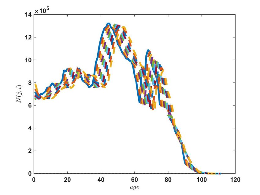
samples the refugee population that arrived in Germany in the years of interest. We use this
information to characterize the incumbent migrant population and the incoming refugees.

                                 Figure 1: Wages since Immigration

    Figure 1 displays wages of migrants, relative to natives with the same level of education,
age and family background, as a function of the time since arrival in Germany. It shows
very sizeable initial wage discounts, in the order of 30% for economic immigrants from poor
countries, and in excess of 40% for political asylum seekers, with very significant conver-
gence towards native German wages over time, especially for the economic migrants, but
at much slower speed for political refugees.2 The availability of rich micro data on migrant
labor market outcomes is an important benefit of analyzing the German experience in the
context of world-wide immigration flows in the last five years. Equipped with these key em-
pirical ingredients we simulate the macroeconomic and distributional impacts of the recent
migration wave. We feed into our model the actual evolution of the domestic and migrant
population (the high migration scenario), as well as two counterfactual scenarios in which we
either fix migration flows to relatively low average levels (the baseline scenario) or only let
political refugees in-migrate (the refugee migration scenario). We obtain three main quanti-
tative findings. First, gross wages of unskilled natives deteriorate, on account of increased
competition on the labor market from equally unskilled refugees. This effect is partially
offset by lower effective contributions to social security; thus net wages of low skilled natives
decrease throughout our entire projection period. Furthermore, taxes increase to finance ad-
ministrative expenditures and transfers to low skilled refugees. Thus, low skilled individuals
currently alive and born in the future experience welfare losses. Second, medium and high
   2
     The much slower convergence among the asylum seekers might not be due to slow productivity conver-
gence, but also reflect restricted access to the German labor market by this group stemming from administra-
tive hurdles described in section 3. It could also stem from reduced incentives to accumulate Germany-specific
human capital since political refugees face a much larger probability of return migration.

                                                      3
skilled natives experience significant welfare gains. Third, the aggregate gains, measured as
consumption equivalent variation, are much larger than the aggregate losses. This suggests
that a compensation of low skilled natives is possible.
    Based on these results our answer to the question motivating this paper is that Germany
should not have built a new wall once transitional dynamics and fiscal and general equilibrium
consequences from the refugee wave in 2015-2018 are taken into account. This is true even
from the perspective of the native low-skilled population, which is most severely subjected
to the migrant competition on the German labor market, but only if this population group is
compensated for their net wage losses using the gains of the rest of the German population.

2    Related Literature
Our work relates to four strands of the literature. First, we build on a large literature
studying the effects of immigration on incomes and welfare of natives. An early influential
paper is Borjas (1999) who shows that an influx of immigrants into a host country (the
U.S. in his context) leads to redistribution among natives towards capital income and an
overall net benefit to native households which Borjas calls the ’Immigration Surplus’. It
emerges as long as capital and (immigrant) labor are not perfect substitutes in production.
Ben-Gad (2004) extends the analysis to endogenous labor supply and capital accumulation
and finds a smaller immigration surplus to the U.S. The same effect of an inflow of labor
will be present in our analysis, and it dampens the long-run decline in the labor force
due to the demographic transition of the native population. Motivated by the evidence in
Borjas (2003) subsequent papers assume imperfect substitution among workers with different
characteristics so that immigration lowers the wages of competing workers. Ben-Gad (2008)
allows for heterogeneous skills and concludes the immigration surplus is maximized with
skilled immigration due to complementarity between skilled labor and capital. In a study for
Germany D’Amuri, Ottaviano, and Peri (2010) show that the pre-2010 inflow of immigrants
leaves wages and employment levels of natives broadly unaffected; incumbent immigrants
are adversely affected by the inflow of new migrants. Felbermayr, Geis-Thöne, and Kohler
(2010) and Ottaviano and Peri (2012) largely confirm these conclusions. In our model we
take these relative gross wage responses into account by allowing for a flexible substitution
structure across skill and nationality groups in aggregate production. This approach is
subject to the criticism by Dustmann, Schonberg, and Stuhler (2016) who argue that the

                                              4
underlying assumption that migrants can be sorted into conventional experience-, education-
and nationality cells might be invalid, a concern we address through sensitivity analyses.3
    Second, our paper is related to the literature on assimilation of migrants. Borjas (1985)
emphasizes the problem of (positive) selection of immigrants who stay in a given country for
estimates of assimilation speeds. More recently, the work by Weiss, Sauer, and Gotlibovski
(2003) and Eckstein and Weiss (2004) emphasizes the adjustment of occupational choices
and human capital formation for wage growth of immigrants to Israel. Dustmann and
Preston (2012) point out an initial skill degradation among immigrants upon arrival into
host countries and Lessem and Sanders (2019) find skill upgrading of immigrants over time,
emphasizing the role played by language skill in this process.4 Motivated by this evidence
we capture assimilation in a reduced form way by allowing the conditional productivity
of immigrants to increase with time since immigration, by estimating assimilation speeds of
wage processes between different groups of immigrants, based on the data shown in Figure 1.
    Third, regarding the fiscal effects of migration we follow Storesletten (2000), who analyzes
the impact of immigration to the U.S. from 1960-1990 in a general equilibrium overlapping
generation economy such as ours. The key finding is that only medium- and high-skilled im-
migration can ease the fiscal burden in the country, whereas low-skilled immigration cannot.
In the context of the ageing population of Japan, Imrohoroglu, Kitao, and Yamada (2017)
reach similar conclusions. Chojnicki, Docquier, and Ragot (2011) perform a retrospective
analysis of the immigration wave of 1945-2000 to the U.S. and conclude that welfare gains
could have been achieved for natives had the past immigration to the U.S. been dominantly
high-skilled. Similarly, the findings of Guerreiro, Rebelo, and Teles (2019) suggest that free
immigration is welfare-maximizing for natives if immigrants can be excluded from the so-
cial welfare system. Finally, using SOEP data Kirdar (2012) estimates the fiscal impact of
immigration on Germany in the presence of an endogenous return migration choice.5
    3
      Llull (2018) observes that imperfect substitutability across workers is an endogenous outcome of het-
erogenous education, labor supply and career choices of natives and incumbent immigrants to show that
natives who are close competitors of immigrants are adversely affected. Similarly, Colas (2019) argues that
natives and old immigrants respond to new immigrants by internally migrating to different labor markets,
and Burstein, Hanson, Tian, and Vogel (2017) analyze how these adjustments vary across tradeable and
non-tradeable sectors.
    4
      Lagakos, Moll, Porzio, Qian, and Schoellman (2018) show that returns to experience accumulated in the
birth country of a migrant before coming to the U.S. are positively correlated with birth-country GDP per
capita. Heise and Porzio (2019) document that even 25 years after the German reunification, real wages in
the East are still 26% lower than in the West.
    5
      A related recent literature uses frictional labor market models and stresses positive effects on immigration
on host economies through endogenous job creation, see e.g. Chassamboulli and Palivos (2014), Nanos and
Schluter (2014), Moreno-Galbis and Tritah (2016), Battisti, Felbermayr, Peri, and Poutvaara (2018) and
Iftikhar and Zaharieva (2019).

                                                        5
Finally, this paper contributes to studies on the impact of the most recent immigration
wave into the European Union, and into Germany specifically. Kancs and Lecca (2018)
analyze alternative refugee integration scenarios for the period 2016-2040 to show that full
repayment of investment in refugees’ integration is achieved in 9 to 19 years and that im-
migration has a positive growth effect on the German economy.6 Scharfbillig and Weissler
(2019) find no evidence that immigrants displace employment of natives but that employ-
ment of incumbent migrants is adversely affected. Their results suggest that natives and
immigrants are imperfect substitutes in production despite having similar qualifications,
whereas the degree of substitution between asylum seekers and other migrant residents of
Germany is higher, which is a key ingredient in our quantitative model.7

3       Institutional Background
In this section we give a brief description of the historical and institutional background of
the large migration inflow in 2015-16. The goal is not to provide a comprehensive review,
but rather give the background for justifying key modelling assumptions in the quantitative
model. More than 50% of the increase in migrants in 2015 and 2016 stems from political
refugees originating in Syria. The Syrian civil war officially began on March 15, 2011.
Political asylum seekers started arriving in numbers via land and sea in Europe in 2013,
and in 2015 the crisis reached its peak when the EU received more than one million asylum
applications from Syria alone. Germany was the main destination country for these refugees.
Chancellor Angela Merkel announced in August 2015 a temporarily suspension of the EU
Dublin regulations which required refugees to apply for asylum in the country to which they
arrive first. In September 2015 Germany agreed to let refugees from Hungary enter Germany.
    As the flow of new asylum seekers subsided in 2017, the focus of policy shifted towards
the integration of these refugees into the German labour market. In August, 2016 the
Prior Review policy that restricted the access of the immigrants to the labour markets was
suspended until August of 2019. In June 2019 “The Alien Employment Promotion Act”
was adopted to promote assistance with asylum procedures and integration into the labour
market. Whereas officially recognized political refugees (those having been granted asylum)
have unrestricted access to German job market and have the same rights as German citizens,
asylum seekers cannot access the labour market during the first three months of their arrival
in Germany. After this waiting period is over access to the labour market is granted with
    6
    Related, Stähler (2017) studies the macroeconomic effects of (failed) integration.
    7
    Further, Dehos (2017) finds a positive association between refugees’ inflow during 2010-2015 and non-
violent property crimes while Sola (2018) concludes that the refugee crisis of 2015 affected the concerns of
the public regarding immigration in the short-run.

                                                     6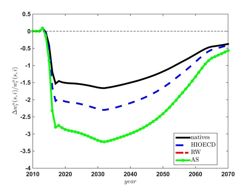
restrictions. In order to get a work permit the asylum seekers must have a job offer and
the German job centers responsible for administering German labour market law check that
neither an EU citizen and nor a non- EU citizen with a residence permit is displaced as
a result of the hiring of the asylum seeker. All asylum seekers are barred from taking up
self-employment for the entire duration of their asylum procedure. Overall, these restrictions
negatively impact both employment opportunities of asylum seekers and the wages they can
earn. As a consequence, wages and earnings of these individuals are initially low, as figure 1
in the introduction shows.
    Finally, in order to assess the fiscal consequences of the recent migration wave, it is
important to assess the extent to which migrants qualify for social assistance. Asylum Seekers
are provided social and medical benefits in accordance with the Asylum-Seekers’ Benefits
Act. Benefits include food, housing, heating, healthcare, personal hygiene, assistance in
sickness, pregnancy and birth as well as household durables and consumables. In October,
2015 the level of social benefits were raised and ’in kind’ benefits were substituted by ’in
cash’ benefits. Furthermore asylum seekers are entitled to standard social benefits and full
healthcare after receiving social benefits under Asylum Seekers’ Benefits Act for 15 months.
Thus, it is a fairly accurate approximation of reality to assume that asylum seekers are
eligible for the same type of social assistance payments as natives, certainly after an initial
period in which these benefits are moderately lower. For a refugee (i.e. a successful asylum
applicant) the same statement applies.
    Against this background, and motivated by the massive inflow of migrants into Germany
in 2015-16 into a labour market characterized by an ageing workforce, we now develop first a
simple model to study the qualitative impact of these developments, before quantifying them
in a more realistic version that allows us to capture the institutional details of Germany in
this period more accurately.

4    Simple Model
We now develop an OLG model with two-period lived households whose basic structure will
also form the foundation for the quantitative model in the next section. The purpose of
this simple model is to clarify the main trade-offs from the recent migration inflows. On
one hand, the asylum seeking immigrants are on average young, and thus help to stabilize
social security budgets. On the other hand, at least initially these migrants have low labor
productivity in the German labor market and the migration system has to be administered
which is costly.

                                              7
Competitive firms operate a neo-classical technology that employs capital and three types
of labor inputs. There are high-skilled (hi) native (na) workers and low skilled workers (lo)
which might either also be natives or come from a per period inflow of foreigners (f o). These
three different groups of workers are assumed to be imperfect substitutes in production.
This structure permits us to display three main effects of an inflow of migrants on gross
wages: First, it increases the relative scarcity of high skilled workers, which, in a model with
imperfect substitutability, increases relative wages of the high skilled and reduces wages of
low-skilled workers. Second, if low-skilled natives and low-skilled foreigners are imperfect
substitutes, an increase in migration raises the relative wage of low-skilled natives. And
finally, an inflow of workers increases the overall supply of labor which, in general equilibrium,
decreases the overall wage level.
    We assume that the economy is ageing, modelled through an exogenous population
growth rate γ n < 1 of the native population. In addition, in every period a number of
young migrants enter the country, shifting the demographic composition of the population
towards younger individuals. In retirement, households earn a social security income, which
is related to past contributions in a Bismarckian pay-as-you-go (PAYGO) pension scheme.
Pension payments in the PAYGO system are financed by levying the contribution rate τ on
labor income of young workers. This structure gives rise to an additional effect of migration
beyond the impact on wages of natives: it increases the population growth rate and thus the
fraction of the young in the population, thereby raising, ceteris paribus, the implicit rate of
return of the pension system.

4.1    Population
There are two-period lived households. We denote by Nt (0) the size of the period t young
population and by Nt (1) the size of the old. We ignore mortality risk, thus Nt+1 (1) = Nt (0).
The young population in each period t consists of native high skill workers, Nt (0, hi, na),
and low skill native- and foreign-born workers Nt (0, lo) = Nt (0, lo, na) + Nt (0, lo, f o). There
is a constant share ω of high skilled workers in the native population, thus Nt (0, hi, na) =
ωNt (0, na) and Nt (0, lo, na) = (1 − ω)Nt (0, na). The population grows at an exogenous
rate γt and thus the young population in t is given by Nt (0) = γt Nt−1 (0).
    The population growth rate γt is determined jointly by the fertility rate of the native
population and the migration rate of individuals from abroad. Let γtn denote the birth rate
of the native population; we assume that once migrants enter the country, they possess the
same fertility rate as native individuals. We further express the exogenous migration flows

                                                8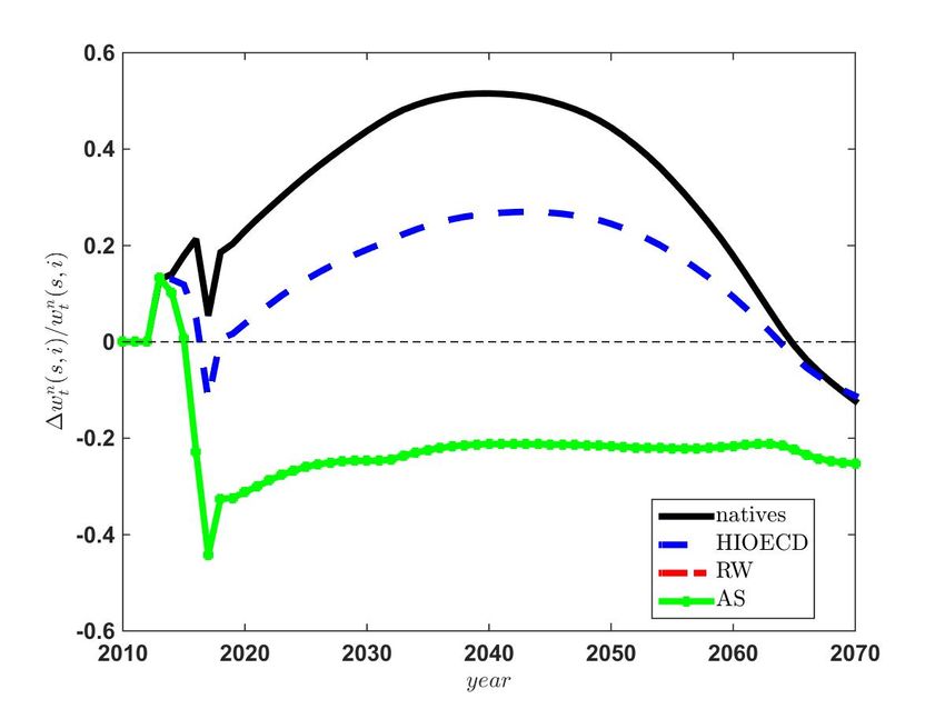
as a share of the population stock of the young population in the previous period,

                                    Nt (0, lo, f o) = µt Nt−1 (0)

Combining these two assumptions yields

                          Nt (0) = γtn Nt−1 (0) + Nt (0, lo, f o)
                                  = (γtn + µt ) Nt−1 (0) = γt Nt−1 (0).

Therefore the population growth rate γt = γtn + µt is the sum of the fertility rate γtn of
individuals living in the country when young, and the migration rate µt ; a positive immigra-
tion µt > 0 then acts like an increase in the fertility rate of the economy.

4.2     Technology
Production takes place with a nested CES-Cobb-Douglas production function of form

                                          Yt = Ktα Lt1−α                                    (1)

where                                                      11
                                       1− 1          1− 1

                           Lt = Lt (lo) σlh + Lt (hi) σlh 1− σlh .                          (2)

and
                                          1− σ 1                1− σ 1
                                                                         11
                                                                         1− σ
                     Lt (lo) = Lt (lo, na)     nf + Lt (lo, f o)     nf       nf            (3)

where σlh is the elasticity of substitution between skilled and unskilled labor, and σnf is the
elasticity of substitution between low-skilled labor supplied by natives and migrants. Notice
that Lt (s, i) are efficiency weighted units of labor with productivity differences across types
of workers described next. Finally, the depreciation rate of capital is denoted by δ = 1.

4.3     Households
Households work one unit of time when young and have skill-specific (s ∈ {lo, hi}) labor
productivity (s, i) that also depends on their migratory origin i ∈ {na, f o}. We normalize
(hi, na) = 1. The group-specific wage per unit of time is denoted by wt (s, i), on which
individuals pay social security contributions at rate τt . When young they consume ct (0, s, i)
and save at+1 (s, i). Assets earn a gross risk-free interest rate Rt+1 . When old they receive
an exogenous retirement income bt+1 (s, i), identical across all workers within a group s, i,
and consume ct+1 (1, s, i). The budget constraints in the two periods of life for workers in

                                                  9
group s, i, are thus given by
ct (0, s, i) + at+1 (s, i) = wt (s, i)(1 − τt ) (4a)
ct+1 (1, s, i) = at+1 (s, i)Rt+1 + bt+1 (s, i). (4b)
Households born in period t of type (s, i) have logarithmic preferences over consumption,
discount the future with factor β. Thus, their lifetime utility function Ut (s, i) given by
Ut (s, i) = ln(ct (0, s, i)) + β ln(ct+1 (1, s, i)). (5)
4.4 Government
The government organizes a PAYG pension system. We assume that pensions of workers of
group i are proportional to their wages when young, where the replacement rate ρt determines
the size of the social security system, and is assumed to be constant across all groups:
bt (s, i) = ρt τt−1 wt−1 (s, i). (6)
Note that the pension system is organized as a Bismarckian system in which benefits are
closely tied to past contributions, which is an accurate approximation of the actual German
system.8 Also note that ρt can be interpreted as the internal gross return of the pension
system since we can rewrite equation (6) as
bt (s, i)
ρt =
τt−1 wt−1 (s, i)
In addition, the government has to finance the bureaucracy in charge of integrating migrants
into Germany. We assume that per migrant a resource cost of κ̃t τt wt is required to administer
the migration system. These resource costs constitute lost output rather than transfers, and
for analytical convenience we express them as a share κ̃t of tax payments. The total cost for
migrants then depends on the number of migrants, and is given by
κ̃t τt wt Nt (0, lo, f o) = κt τt wt Lt
where κt = κ̃t Nt (0,lo,f
Lt
o)
. Written in this way, the cost κt captures both the cost per migrant
κ̃t , a parameter of the model, and the effect of an increase in the number of migrants (as
parameterized by µt ), since the ratio Nt (0,lo,f
Lt
o)
is strictly increasing in µt .
8
The German legislation does not feature dependency on τt−1 , but note that this is just a rescaling of
the replacement rate because we could equivalently write bt (s, i) = ρ̃t wt−1 (s, i)
10Finally, we assume that the budget of the government is balanced in every period, which
requires that the sequence of payroll tax rates {τt } satisfies:
X X X X
τt wt (s, i)Nt (0, s, i) = ρt τt−1 wt−1 (s, i)Nt (1, s, i) + κt τt wt Lt .
s∈{hi,lo} i∈{na,f o} s∈{hi,lo} i∈{na,f o}
(7)
By assumption there are no high-skilled migrants in the model, and thus Nt (0, hi, f o) =
Nt (1, hi, f o) = 0. Simply put, given labor income taxes {τt } and costs for administrating
migration (as parameterized by κt ), the social security replacement rate ρt adjusts to changes
in the demographic composition of the population, to ensure government budget balance.9
4.5 Characterization of Equilibrium
We relegate a formal definition of the competitive equilibrium to appendix A. As is common
in neoclassical growth models, the key variable describing the dynamics of the competitive
equilibrium is the capital-labor ratio kt = Kt
Lt
. Starting from an arbitrary initial capital K0
and for an exogenous sequence of skilled and unskilled labor determined by fertility and
migration rates as well as exogenous policy (characterized by social security replacement
rates), once the dynamics of capital and thus the capital-labor ratio is determined, factor
prices, relative wages of each group, factor demands and consumption allocations of all
private households follow directly from the firm’s optimality conditions and the household
budget constraints. The dynamics of the capital labor ratio itself is determined from private
household savings decisions and the asset market clearing condition.
We will proceed with the analysis of the model “from the back”, first characterizing
wages for a given sequence of the capital-labor-ratio, then demonstrating that in the model
all households optimally choose the same saving rate, which then in turn determines the law
of motion for the capital-labor ratio. We finally provide comparative statics with respect to
the size of migration flows, as summarized by the migration rate µt .
4.5.1 Firm Optimization and Equilibrium Wages
The representative firm hires three types of labor Lt (hi), Lt (lo, na), Lt (lo, f o), combines them
into a labor composite Lt and uses this labor and capital Kt to produce output. Profit
maximization implies that the gross return on capital and the wage per unit of the labor
9
For analytical convenience, in the simple model we consolidate the social security and general government
revenue budget; the quantitative model will separate these two budgets, as is realistic for the German case.
11composite equal the marginal products of capital and labor, respectively:
1 + rt = Rt = αktα−1 (8)
wt = (1 − α)ktα . (9)
Furthermore, the wage per unit of time for a worker of type (s, i) is determined by the product
of its labor efficiency units (s, i), the wage per efficiency unit of the labor composite wt and
the marginal product of labor of type (s, i) in producing the labor composite Lt , that is,
∂Lt
wt (s, i) = wt · (s, i) · (10)
∂Lt (s, i)
Exploiting equations (2) and (3) yields as wages (and thus labor incomes) as functions
of the common wage per labor efficiency units as well as the relative scarcity of different
demographic groups, whose impact is controlled by the substitution elasticities between
skilled and unskilled labor σlh and between unskilled labor of natives and migrants σnf .
σ1
Lt lh
wt (hi) = wt · (11)
Lt (hi)
σ1 1
Lt lh Lt (lo) σnf
wt (lo, i) = wt · (lo, i) · · (12)
Lt (lo) Lt (lo, i)
Exploiting the market clearing conditions (29) and (30) and the demographic relationships
to express labor efficiency units of the different groups in terms of demographic variables
gives the following:
Proposition 1. Equilibrium wages of the different groups are determined as
wt (hi) = wt Whi (µt /γtn )
wt (lo, na) = wt Wlo (µt /γtn ) · Wna (µt /γtn )
where the exogenous demographic factors Whi (µt /γtn ), Wna (µt /γtn ) are increasing in µt /γtn
and Wlo (µt /γtn ) is decreasing in µt /γtn . The wage wt per labor efficiency unit is a strictly
increasing function purely of the aggregate capital-labor ratio.
124.5.2 Household Optimization
To derive the equilibrium dynamics of the capital-labor ratio it is useful to restate the
household maximization problem in terms of household saving rates
at+1 (s, i)
st (s, i) = (13)
wt (s, i)
With this definition we can rewrite consumption in both periods as
ct (0, s, i) = wt (s, i) [(1 − τt ) − st (s, i)] (14)
ρt+1 τt
ct+1 (1, s, i) = wt (s, i)Rt+1 st (s, i) + (15)
Rt+1
and the objective function of the household becomes
wt (s, i)
Ut (s, i) = (1 + β) ln(wt ) + β ln(Rt+1 ) + (1 + β) ln
wt
ρt+1 τt
+ ln ((1 − τt ) − st (s, i)) + β ln st (s, i) + (16)
Rt+1
This expression clarifies the three forces impacted by population ageing and migration. First,
demographic changes affect general equilibrium aggregate factor prices (wt , Rt+1 ) unless we
analyze a small open economy. Second, it changes relative wages of the different population
groups, as summarized by proposition 1. Third, it changes the relative return on the social
security system measured by Rρt+1 t+1
, and with it, potentially the optimal saving decisions of
households. With log-utility the optimal saving rate is independent of the first two forces.
Taking first order conditions with respect to (16) gives the optimal saving rate as
ρt+1
β(1 − τt ) − τ
Rt+1 t
st (s, i) = (17)
1+β
Note that the saving rate is identical across all population groups and only depends on
the fiscal side of the model characterizing the PAYGO social security system. The only
remaining endogenous variable in the saving rate and thus in the welfare of a given generation
is the relative return of the social security system Rρt+1
t+1
. Using the budget constraint of the
13government (7) and noting that Nt+1 (i, 1) = Nt (i, 0) we have
P
ρt+1 τt+1 s,i wt+1 (s, i)Nt+1 (s, i, 0) − κt+1 wt+1 Lt+1
= P
Rt+1 τt Rt+1 s,i wt (s, i)Nt (s, i, 0)
τt+1 (1 − κt+1 )wt+1 Lt+1 (1 − κt+1 )τt+1 wt+1 L
= = γ
τt Rt+1 wt Lt τt Rt+1 wt t+1
L
where γt+1 = LLt+1
t
is the growth rate of aggregate labor supply in efficiency units, and
a function purely of the exogenous demographics of the model, as lemma 1 below shows.
The general equilibrium term Rwt+1t+1
wt
is still endogenous and depends on the dynamics of
the capital-labor ratio. To establish a benchmark we first characterize the saving rate and
welfare in a small open economy where the interest rate R is constant and exogenous, which,
from the firm optimality conditions, implies a constant exogenous wage wt = w per labor
efficiency unit and a constant exogenous capital-labor ratio.
4.5.3 The Savings Rate and Welfare in Partial Equilibrium (Small Open Econ-
omy)
With an exogenous interest rate R the term Rwt+1t+1
wt
in equation (18) is exogenous and equals
wt+1
Rt+1 wt
= R1 . The following proposition immediately follows from equations (17) and (16):
Proposition 2. In a small open economy, the equilibrium saving rate and welfare of an
individual of type (s, i) born at time t are given by
L
γt+1
β(1 − τt ) − (1 − κt+1 )τt+1 R
st (s, i) = = st
1+β
wt (s, i)
Ut (s, i) = (1 + β) ln(w) + β ln(R) + (1 + β) ln
wt
L
γt+1
+ β ln(β) − (1 + β) ln(1 + β) + (1 + β) ln 1 − τt + (1 − κt+1 )τt+1
R
4.5.4 The Dynamics of the Capital-Labor Ratio in General Equilibrium
In general equilibrium the ratio Rwt+1
t+1
wt
is endogenous and requires one to solve for the dynam-
ics of the capital-labor ratio. The market-clearing condition on the capital market implies
X X
Kt+1 = at+1 (s, i)Nt (0, s, i) = st (s, i)wt (s, i)Nt (0, s, i) = st wt Lt
s,i s,i
14and thus
Kt+1 (1 − α)ktα
= kt+1 = st L
(18)
Lt+1 γt+1
α
wt+1 (1 − α)kt+1 (1 − α)st
= α−1 α
= L
(19)
Rt+1 wt αkt+1 (1 − α)kt αγt+1
ρt+1 τt+1 (1 − κt+1 )wt+1 L (1 − κt+1 )τt+1 (1 − α)st
τt = γt+1 τt = (20)
Rt+1 τt Rt+1 wt α
Equations (17) and (20) can be solved for the saving rate in general equilibrium, which in
turn determines general equilibrium welfare. These results are summarized in the following
Proposition 3. The general equilibrium saving rate and welfare of an individual of type
(s, i) born at time t are given by
αβ(1 − τt )
st (s, i) = st = (21)
α(1 + β) + (1 − α)(1 − κt+1 )τt+1
wt (s, i)
Ut (s, i) = (1 + β) ln(wt ) + β ln(Rt+1 ) + (1 + β) ln
wt
α + (1 − α)τt
+ β ln(β) + (1 + β) ln(1 − τt ) + (1 + β) ln
α(1 + β) + (1 − α)(1 − κt+1 )τt+1
4.6 Comparative Statics: An Increase in the Migration Rate µ
In this subsection we derive the comparative statics of the model with respect to the mi-
gration rate µt and the fertility rate (population growth rate) γtn of the native population.
From propositions 2 and 3 we know that these are completely determined by the demographic
factors driving relative wages Whi (µt /γtn ), Wna (µt /γtn ) as well as the growth in aggregate la-
L
bor γt+1 (µt , γtn ). The following lemma, proved in appendix A, summarizes the impact of
migration and fertility rates on these exogenous demographic factors.
Lemma 1. Consider a change in the migration and/or native fertility rate (µt , γtn )
1. The relative wage factors Whi (µt /γtn ), Wna (µt /γtn ) are strictly increasing in µt /γtn and
Wlo (µt /γtn ) is strictly decreasing in µt /γtn .
L
2. The growth rate of aggregate labor γt+1 (µt , γtn ) is strictly increasing in µt and γtn if the
changes in µt , γtn are permanent. The share of migrants in labor Nt (0,lo,f Lt
o)
and thus κt
is strictly increasing in µt if the changes in µt , γtn are permanent.
Equipped with this result and propositions 2 and 3 we now can state
Theorem 1. Consider an unexpected but permanent increase in the migration rate µt .
151. First consider a small open economy:
(a) Welfare of all young native households is negatively impacted by an increase in
the effective cost from migrants κt+1 , positively impacted by an increase in the
γL
relative return on social security t+1
R
, and from the relative wage effect Whi (µt /γtn )
is unambiguously positive for high-skilled natives, but Wlo (µt /γtn ) · Wna (µt /γtn ) is
ambiguous for low-skilled natives.
(b) Therefore as long as migrants are not too costly (κ̃t+1 and thus κt+1 is sufficiently
small), welfare of young high-skilled natives at the time of the migration boom,
Ut (hi, na) increases due to the boom.
(c) The welfare consequences for young low-skilled natives Ut (lo, na) are ambiguous,
but positive as long as their relative wages do not decline too much. This is the
case as long as native and migrant low-skilled labor is sufficiently non-substitutable
relative to skilled vs. unskilled labor (i.e. as long as σnf is sufficiently small
relative to σlh ).
2. In general equilibrium the migration cost and the relative wage effects are identical
to those in the small open economy and the impact on the relative return on social
γL
security t+1
R
is absent. The wage level wt falls and the real return Rt+1 increases, and
the overall general equilibrium effect (1 + β) ln(wt ) + β ln(Rt+1 ) is negative as long as
the capital share α is sufficiently large or the increase in labor in t and t + 1 is of
similar magnitude.10 In this case the welfare consequences from the migration boom
shift down for all groups relative to the small open economy.
The proof follows directly from lemma 1 as well as propositions 2 and 3. A similar
theorem can be derived for a decline in the population growth rate of the native population.
The main upshot of the simple model is that the welfare consequences of the 2015-106
immigration boom will depend on four factors: i) the relative wage effects determined by
the relative substitution pattern of skilled, unskilled native and skilled native labor, ii) the
adjustment of the PAYGO pension system, iii) the costs to administer the migration system
and iv) general equilibrium level effects on wages and interest rates which are likely adverse.
We now seek to quantify these effects in a more realistic large-scale overlapping generations
economy.
10
The appendix provides conditions on the fundamentals for which this is true, and they are easily verifiable
in the quantitative model.
165 The Quantitative Model
The quantitative model we employ is a large-scale overlapping generations model in the tra-
dition of Auerbach and Kotlikoff (1987), but with time-varying, deterministic demographic
structure. The key model ingredients are i) a detailed demographic model that accurately
describes migrant flows into and out of the country, ii) a production technology that allows
for flexible substitution patterns of workers with different migratory background and leads to
relative wages that depend on the relative labor supplies of the different population groups,
iii) a household sector making consumption-savings and labor supply decisions, and iv) a
government that administers the migration system, a basic social safety net, a pay-as-you-go
social security system and that collects taxes.
We now first describe the underlying demographic model that captures the flow of mi-
grants and asylum seekers into Germany. We then turn to the description of the economic
model, its production technology, endowments and preferences of households, as well as gov-
ernment policies. The recursive formulation of the household problem and the definition of
equilibrium is relegated to the appendix.
To provide an overview and set up notation, Table 1, summarizes the state variables used
in the model. We refer to it at various places of the remaining description.
Table 1: List of State Variables
State Var. Values Interpretation
j j ∈ {0, 1, . . . , J} Model Age
s s ∈ {lo, me, hi} Skill (education)
i i ∈ {na, ho, rw, as} Region of Origin
g g ∈ {f e, ma} Gender
m m ∈ {si, co} Marital status
e e ∈ {em, re, rl} Labor Market Status
a a≥0 Assets
5.1 Demographics and Population Flows
We distinguish between the native population and the foreign-born population. Foreigners
are composed of those that entered the country as regular immigrants and those that came
as refugees and are asylum seekers.11 The basic difference between native households and
11
We use the terms “refugees” and “asylum seekers” interchangeably. Empirically the latter group includes
all successful asylum seekers as well as those waiting for a decision of their application, and finally those
that have either been denied protection or lost their humanitarian residence title but remain in the country.
17foreigners is in their labor productivity, their access to government transfers as well as the fact
that labor inputs supplied by natives and foreigners are imperfect substitutes in production.
We consider four population groups, denoted by i ∈ {na, hi, rw, as}, which we also refer
to as “citizenship” (in an economic, not in a legal sense). Within the group of regular
immigrants, we distinguish between the stock originating from high income OECD countries
(ho) and the rest of the world (rw). We assume that each population group is composed
of three education groups, the low, medium, and high skilled, denoted by s ∈ {lo, me, hi}.
Within each group we consider two genders of individuals, g ∈ {f e, ma}, of f emale and male
workers. We assume that mortality and fertility rates are homogeneous across skill groups.
Households are born at age j = 0 and live at most until age J > 0. The number of people
alive at time t of age j from region i and of gender g is denoted by Nt (j, i, g), the number of
people dying between period t and t + 1 and from age j to j + 1 is denoted by Dt+1 (j + 1, i, g)
and the net inflow of immigrants of this group by Mt+1 (j + 1, i, g), which may be negative
in case there is net emigration. We further define by ςt (j, i, g) = 1 − Dt+1 (j+1,i,g)
Nt (j,i,g)
the time-,
age-, population group- and gender-specific survival rate. We restrict survival rates to be
the same across genders, ςt (j, i, f e) = ςt (j, i, ma) = ςt (j, i). Although this is a counterfactual
restriction on demographic dynamics—females have higher survival rates than males—it
significantly simplifies the economic model where we assume that both members of couple
households have the same age and die jointly. Also, denote by µt (j, i, g) = Mt+1 (j+1,i,g)
Nt (j,i,g)
the
net migration rate, i.e., the percentage net addition to the stock of (j, i, g) type individuals
from period t to t + 1.
For most of the analysis we model the dynamics of immigrants into the country in terms
of net flows Mt (j, i, g) and thus implicitly assume that the gross flow is equal to the net flow.
However, two additional model elements concerning asylum seekers deserve mention: some
have to leave the country, and some “assimilate” and become regular rw immigrants. Each
period the stock Nt (j, as, g)ςt (j, as) of asylum seekers that survives to the next period faces
the probability π l of having to leave the country. Those that stay face a probability π ar to
f
assimilate to the rw population group. Denoting by Mt+1 (j +1, as, g) the inflow from foreign
countries to that group, the net immigration flow to group as is thus
f
(j + 1, as, g) − π l + (1 − π l )π ar Nt (j, as, g)ςt (j, as)
Mt+1 (j + 1, as, g) = Mt+1
and therefore
µt (j, as, g) = µft (j, as, g) − π l + (1 − π l )π ar ςt (j, as).
18Likewise, we assume that in each period a fraction π rh of the stock of population group rw
f
assimilates to population group ho. Denoting by Mt+1 (j + 1, rw, g) the inflow from foreign
countries to population group rw, the net inflow to the population group rw is thus
f
Mt+1 (j + 1, rw, g) = Mt+1 (j + 1, rw, g) + (1 − π l )π ar ςt (j, as)Nt (j, as, g)
− π rh ςt (j, rw)Nt (j, rw, g)
and thus
Nt (j, as, g)
µt (j, rw, g) = µft (j, rw, g) + (1 − π l )π ar ςt (j, as) − π rh ςt (j, rw).
Nt (j, rw, g)
f
Correspondingly, denoting by Mt+1 (j + 1, ho, g) the inflow from foreign countries to popula-
tion group ho, the total inflow to the population group ho is
f
Mt+1 (j + 1, ho, g) = Mt+1 (j + 1, ho, g) + π rh ςt (j, rw)Nt (j, rw, g)
and thus
Nt (j, rw, g)
µt (j, ho, g) = µft (j, ho, g) + π rh ςt (j, rw) .
Nt (j, ho, g)
The dynamics for the size of each population group is then determined according to:
Nt+1 (j + 1, i, g) = Nt (j, i, g) − Dt+1 (j + 1, i, g) + Mt+1 (j + 1, i, g)
= Nt (j, i, g) (ςt (j, i) + µt (j, i, g)) , (22)
with terminal condition Dt+1 (J + 1, i, g) = Nt (j, i, g) and Mt+1 (J + 1, i, g) = 0, that is, at age
J all individuals die and no more migrants enter the country. This concludes the description
of the exogenous mortality and migration processes.
Turning now to fertility, denote by χt (j, i) the time t, age j, group i specific fertility rate.
We assume an exogenous sex ratio at birth and denote by φ the fraction of baby girls (which
is assumed to be constant over time and across population groups). We further assume that
all newborns of group i are natives. We denote by jf the first fertile age of a woman and
by jc the age of completed fertility. The number of native newborns of gender Nt+1 (0, n, g)
19in period t + 1 is then given by
jc
X X
Nt+1 (0, na, f e) = φ χt (j, i) Nt (j, i, f e) (23a)
j=jf i∈{na,ho,rw,as}
jc
X X
Nt+1 (0, na, ma) = (1 − φ) χt (j, i) Nt (j, i, f e). (23b)
j=jf i∈{na,ho,rw,as}
Since all babies born in Germany are treated as natives, the age 0 population in the foreign
population groups are those that migrated from t to t + 1 to Germany as babies, thus
for i ∈ {ho, rw, as} we have
Nt+1 (0, i, g) = Mt+1 (0, i, g).
5.2 Technology
Output Yt is produced with a neoclassical production function that displays constant returns
to scale in capital Kt and a labor aggregate Lt . Firms operate in perfectly competitive output
and factor markets, and thus earn zero profits in equilibrium. Given these assumptions,
without loss of generality we consider the problem of a representative firm. We assume a
Constant Elasticity of Substitution (CES) aggregate production function of the form
11
1− 1
1 1−
Yt = αKt ϑ + (1 − α)(At Lt )1− ϑ ϑ
.
where ϑ is the substitution elasticity between capital and the labor aggregate. Aggregate
labor in turn is a CES aggregate of labor supplied by the different skill groups s ∈ {le, me, hi},
Lt (s) with substitution elasticity σlmh :
1
1− σ 1
1 lmh
1− σ
X
Lt = Lt (s) lmh .
s∈{lo,me,hi}
Labor of skill group s in turn is the CES aggregate of natives and f oreigners with substitution
elasticity σnf giving
1
1− σ 1 1− σ 1
1− σ 1
Lt (s) = Lt (s, na) nf + L̃t (s, f o) nf nf .
With respect to the foreign population stock, we further distinguish between different coun-
tries of origin, and thus the education specific foreign (or immigrant) labor input is disag-
20gregated further with substitution elasticity σhr as
1− σ1 1− 1 1
hr σhr
1− 1
X
L̃t (s, f o) = Lt (s, ho) σhr + Lt (s, i) .
i∈{rw,as}
Note that we thereby assume that conditional on education and experience, population
groups rw and as are perfect substitutes in production.12 As lowest nests we assume perfect
elasticities of substitution across age and gender13 and thus Lt (s, i) = Jj=ja Lt (j, s, i), Lt (j, s, i) =
P
P
g∈{f e,ma} (j, s, i, g)Lt (j, s, i, g). Capital is assumed to depreciate at constant rate δ. The
first-order conditions of the firm problem are provided in Appendix B.
5.3 Households
The recursive formulation of the life-cycle household model is contained in Appendix B. Here
we describe the main elements.
5.3.1 Marital Status
Agents of gender g may either live as singles or as a couple, thus the “marital status”
is m ∈ {si, co}. For simplicity, we assume that marital status is known from the start
of economic live at age ja . We denote by π m (i, g) the exogenous probability of finding a
partner at age ja , which is population group and gender specific. Accordingly, a fraction of
individuals remains single and another fraction forms couples. Thus, there are three types of
households by gender: single females, single males and couples. To reduce the dimensionality
of the state space we assume that couples always feature partners of the same age j and
the same citizenship i. We allow for imperfect assortative matching across skill groups s.
We further assume that there is no possibility of divorce and married households live as a
couples until they die.
5.3.2 Timing of Work and Retirement
Agents work from age ja until at most the mandatory retirement age jr . At age ja the
idiosyncratic elements of the wage process (j, s, i, g) realize. Skill s is exogenously given at
economic birth and we do not consider any inter-generational spill-overs of skills. There are
12
This is due to data limitations. We have too few observations on asylum seekers in the data, which
inhibits the estimation of a substitution elasticity parameter.
13
Again, this assumption is due to data limitations, as the production function is estimated at the level
of the defined groups, and there are too few observations to make the production function more flexible.
21three skill levels, low, medium and high, s ∈ {lo, me, hi}. While agents know their skill lev-
els already at age ja , for an initial working period j ∈ {ja , . . . , js } agents of skill s lose some
time endowment %(s) ∈ (0, 1), which stands in for time spend on formal education, which
increases in the skill level, jhi > jme > jlo = ja − 1, i.e., the low skilled have full time endow-
ment from age ja onwards. Labor supply can be chosen from the discrete set {l1 , . . . , ln },
where l1 = 0. Asylum seekers are not allowed to work for the first three months after arrival.
We model this by adjusting the set of possible labor supply choices to ${l1 , . . . , ln } and
calibrate $ = 34 . There is an early retirement window, i.e., for age j ∈ {je , . . . , jr − 1} agents
can choose to retire early. For simplicity, we assume joint retirement by couples. We denote
the employment status by e ∈ {em, re, rl}, where em is employment, re is early and rl is
late (or regular) retirement, both of which we take to be an absorbing state.
5.3.3 Endowments
Agents (males or females) are endowed with one unit of productive time. An agent of skill s,
age j, “citizenship” i, gender g earns an hourly gross wage of
wt (s, i)(j, s, i, g) (24)
where wt (s, i) is determined from the firm side and (j, s, i, g) is age, skill, nationality and
gender specific productivity, , cf. Section 5.2.
In case individuals choose zero hours (l = 0) they are labeled as “unemployed” and receive
asset-tested lump-sum social assistance pay. Social assistance pay further depends on family
status and the number of children in a household. To capture these institutional features
we denote social assistance pay by but (a, n, m) where a are household asset holdings, m is
marital status, n is the number of children living in the household. Means testing is such
that transfers are not paid out if household assets exceed threshold at (m, n), which depends
on marital status and the number of children in the household, thus
b̄u (m, n) if a(·) ≤ a (m, n)
u t t
bt (a, n, m) = (25)
0 otherwise.
In retirement, agents earn a retirement income, which depends on all fixed observable
characteristics that measure productivity, s, i, g. According to legislation there are early and
late retirement adjustment factors according to which pension payments are adjusted by the
actual age of retirement. We approximate this by letting retirement fall into two brackets
for early and late (respectively regular) retirement. Thus, if the age of retirement falls in
22the bracket [je , jl ) then the retirement state is re, if it is in bracket [jl , jr ] the retirement
state is rl. The elements of pension benefits accruing at the individual level are stored in
variable p(s, i, g, e), where it is understood that p(·) = 0 for e = em. Pension benefits are
further scaled by an aggregate factor υtp , which clears the aggregate pension budget in each
period, cf. Section 5.4. We additionally introduce social assistance pay in old-age at some
level bpt (m)(a, n, m), which, as the social assistance pay during the working period, is means
tested, cf. equation (25), depends on marital status, the number of children co-residing with
retired households and grows exogenously at rate λ.14 Thus, pension benefits are given by
0 for e = em
bpt (a, n, s, i, g, m, e) = υtp · p(s, i, g, e)+ (26)
max{bpt (a, n, m) − υtp · p(s, i, g, e), 0} otherwise.
Agents start their economic life with zero assets. From then on they have access to a
risk-free savings technology with gross interest rate rt . Assets of couples are pooled. In case
singles or both members of a couple die, assets are confiscated and redistributed as accidental
bequests, lump-sum within population subgroups j, s, i to all households of that group. We
denote these transfers from accidental bequests by trt (j, s, i).
For asylum seekers, we distinguish between the first period in which they are asylum
seekers and all other periods in which they are accepted or tolerated (we do not distinguish
between those).15 We denote the seeking state by indicator 1a , which is equal to one in
the first period after arrival. As asylum seekers they are allowed to work, except for the
first three months. Accordingly the labor market states are li ∈ 43 · {l1 , . . . , ln }. Working
is subject to the priority review, which decreases their productivity and is reflected in our
productivity estimates. If they do not work, then they receive transfer payments bat (n, m),
which as the social insurance payments, are means tested and adjusted to household size.
If they do work, transfer payments are reduced one for one. At the end of the first period,
conditional on surviving to the next period they face a probability π l with which they have
to leave the country and, conditional on staying, a probability π ar with which they assimilate
to the foreign population group rw. The remaining fraction (1 − π l )(1 − π ar ) stays in state as
as accepted or tolerated asylees and the seeking indicator 1a accordingly switches to zero.
From now on, asylees who remain in state as have full access to the German social insurance
scheme but their labor productivity is lower than for population group rw. At the end of
14
The age of completed fertility in the data is age jc = 50. Since own households form at the age of 17,
some children may live in households that are already retired.
15
According to factual legislation, some are non-accepted asylees but are tolerated to stay. Of others the
status may still be pending after one year. Economically, there is little difference across these different types.
23You can also read