Ifo WORKING PAPERS 335 2020
←
→
Page content transcription
If your browser does not render page correctly, please read the page content below
ifo                                   335
                                     2020
WORKING                              August 2020

PAPERS
 The ifo Tax and Transfer
 Behavioral Microsimulation
 Model
 Maximilian Blömer, Andreas Peichl
Imprint:

ifo Working Papers
Publisher and distributor: ifo Institute – Leibniz Institute for Economic Research at the
University of Munich
Poschingerstr. 5, 81679 Munich, Germany
Telephone +49(0)89 9224 0, Telefax +49(0)89 985369, email ifo@ifo.de
www.ifo.de

An electronic version of the paper may be downloaded from the ifo website:
www.ifo.de
ifo Working Paper No. 335

   The ifo Tax and Transfer Behavioral Microsimulation Model

                                            Abstract

This paper describes the ifo Tax and Transfer Behavioral Microsimulation Model (ifo-
MSM-TTL), a policy microsimulation model for Germany. The model uses household
microdata from the German Socio-Economic Panel and firm data from the German
Linked Employer-Employee Dataset. This microsimulation model consists of three
components: First, a static module simulates the effects of a tax-benefit reform on
the budget of the individual household. This includes taxes on income and consump-
tion, social security contributions, and public transfers. Secondly, behavioral labor
supply responses are estimated. Thirdly, a demand module takes into account
possible restrictions of labor demand and identifies the partial equilibrium of the
labor market after the supply reactions. The demand module distinguishes our
model from most other microsimulation tools.

JEL code: D58, H20, J22, J23
Keywords: Tax and benefit systems, labor supply, labor demand, Germany, policy
simulation

             Maximilian Blömer                               Andreas Peichl*
    ifo Institute – Leibniz Institute for          ifo Institute – Leibniz Institute for
            Economic Research                              Economic Research
        at the University of Munich,                   at the University of Munich,
                 HU Berlin,                                University of Munich,
              Poschingerstr. 5                               CESifo, HIS, IZA
          81679 Munich, Germany                              Poschingerstr. 5
         Phone: +49-89-9224-1220                         81679 Munich, Germany
              bloemer@ifo.de                            Phone: +49-89-9224-1225
                                                              peichl@ifo.de

* Corresponding author.
1 Introduction
The ifo Microsimulation Model (ifo-MSM), developed at the ifo Institute, has two main
variants: A model used especially for tax policies building on administrative tax return
data (ifo-MSM-TA) and a behavioral microsimulation model used for tax and transfer
policy evaluation and labor supply simulation building mainly on the GSOEP data
(ifo-MSM-TTL).1 This paper describes the current version of the latter variant, the Tax
and Transfer Behavioral Microsimulation Model (ifo-MSM-TTL).2
Note that the ifo Tax and Transfer Behavioral Microsimulation Model has sister
projects at IZA Bonn and ZEW Mannheim which share part of the underlying code
base.3 This documentation provides a largely technical description of the latest version
of the ifo Microsimulation Model and its different modules. While large parts of the
code have been revised and new policies have been included, the basic structure of the
model has been maintained. Hence, this documentation draws heavily from Peichl et al.
(2010b) and Löffler et al. (2014a).
The ifo Microsimulation Model consists of three core components. The basis is a static
microsimulation model that incorporates the complex German tax and benefit system
for the years 1984 to 2020. The second module is a micro-econometrically estimated
labor supply model, which takes into account behavioral reactions to reforms of the
tax-benefit system. The third component is a labor demand module, which completes
the analysis of the labor market and allows a global assessment of the effects of policy
measures. Finally, the ifo Microsimulation Model incorporates a comprehensive output
module that allows analyzing the likely effects of policy reforms in various illustrative
ways. Components one and two are based on data from the German Socio-Economic
Panel (GSOEP), a representative panel study of private households in Germany. Supple-
mentary information can be drawn from the German Income and Expenditure Survey
(EVS) and the Income Tax Return Data (FAST). The demand module uses German
Linked Employer-Employee Data from the IAB (LIAB).
Microsimulation Models (MSM) have become one of the standard analytical tools in
the field of applied welfare and distributional analysis. The main feature of a microsim-
ulation approach is the partial equilibrium analysis that simulates the effects of policy
1
For recent applications using ifo-MSM-TA, see e.g. Dorn et al. (2017a,b) and Fuest et al. (2017). For
applications using ifo-MSM-TTL see Section 7 of this documentation. An application where both
variants of the model have been used can be found in Blömer et al. (2019a).
2
In the following the ifo-MSM-TTL will also be called simply “ifo Microsimulation Model”.
3
The sister projects are branded IZAΨMOD and the ZEW Microsimulation Model. The model de-
velopment started in the mid 2000s at FiFo Cologne (see Peichl and Schaefer, 2009) and continued
later first at IZA and then at ZEW, see Peichl et al. (2010b) and Löffler et al. (2014a). The authors
would like to thank everybody who has been helping to develop this microsimulation model and con-
tributed to the code base over the past years, especially Florian Buhlmann, Max Löffler, Nico Pestel,
Sebastian Siegloch, Eric Sommer and Holger Stichnoth for valuable contributions. We thank the
Gesellschaft zur Förderung der wirtschaftswissenschaftlichen Forschung (Freunde des ifo Instituts)
e.V. for financial support.
2reforms (i.e. changes in tax or benefits) on one side of the market (i.e. households, firms,
individuals). The simulation basically consists of evaluating the effects of a change in
the economic environment of individual agents in terms of welfare or activity (Bour-
guignon and Spadaro, 2006). MSM are based on microdata and therefore account for
heterogeneity of economic agents within the population. Hence, the advantage of MSM
stems from the precise identification of winners and losers of a reform, which allows for
the overall evaluation of welfare effects as well as political economy factors that may
obstruct the implementation.
Within the MSM category, many models are applied to redistribution policies. Tax
models, for example, are widely used to simulate the distributional consequences of a tax
or benefit change among heterogeneous groups of families and to predict the likely costs
to the government of a proposed or hypothetical policy reform (Creedy and Duncan,
2002).
As far as the distributional analysis is concerned, there is a variety of different ap-
proaches. Non-behavioral models, also referred to as arithmetic models, simulate changes
in the real disposable income of individuals or households due to a tax or benefit re-
form under the assumption that behavior is exogenous to the tax and benefit system
(Bourguignon and Spadaro, 2006). Hence, individuals are not allowed to change their
behavior. These models simulate first-round effects only, which comprise immediate
fiscal and distributional changes.
In contrast to arithmetic models, behavioral models take some kind of behavioral re-
sponse of individuals or households into account. Such responses are usually based on the
rationale of utility maximization. Within this approach, labor supply and consumption
are among the types of behavior most frequently included in the analysis. Microe-
conometric labor supply models incorporate a theoretical grounding of the behavioral
response and allow for the modeling of labor supply decisions along the extensive (la-
bor market participation) as well as the intensive (hours worked) margin (Peichl, 2009).
Usually, a labor supply module is either integrated into the microsimulation model or
can be linked to it as an external module.
The simulation steps of the ifo Microsimulation Model are illustrated in Figure 1 and
can be described as follows: First, the database for the year of interest is generated.
Following common practice, we impute non-observed wages with a Heckman procedure
(Heckman, 1979). Secondly, the current tax and benefit system (often called “Status
quo”) is simulated using the modified data. The ifo Microsimulation Model computes
individual tax payments for each case in the sample considering gross incomes and de-
ductions in detail. This way, we obtain disposable income for every household in the
sample. Thirdly, a discrete choice household labor supply model is applied to estimate
the consumption/leisure preferences of each household using the calculated net incomes
and information on working hours. Fourthly, the effects of tax and benefit reforms are
analyzed. The reform will alter net incomes of households (first-round effect), which,
3Estimation of LS module
Tax transfer SQ
SQ × Wages SQ SQ SQ
Hours = Gross incomes Net incomes
Tax transfer Ref
SQ × Wages SQ SQ Ref (MA)
Hours = Gross incomes Net incomes
LS module
Tax transfer Ref
Ref × Wages SQ Ref Ref (LS)
Hours = Gross incomes Net incomes
LD module
Tax transfer Ref
Ref’ × Wages Ref’ Ref’ Ref (LD)
Hours = Gross incomes Net incomes
LS module
Notes: “SQ” denotes the variables (hours, wages and income variables) in the status quo tax and transfer
system. “Ref” denotes the variables in the counter factual reform scenario. “Ref (MA)” denotes the
outcome variables after applying the reform tax and transfer system, without simulating any behavioral
changes (“morning after”). “Ref (LS)” denotes the outcome variables taking labor supply effects (LS)
into account. The labor demand (LD) module iterates LD and LS effects until convergence, resulting in
outcome variables denoted by “Ref (LD)”.
Figure 1: Model Setup and Simulation Steps
in a second step, will induce labor supply reactions following the previously estimated
consumption/leisure preferences which are assumed to be constant. Next, the labor
demand module is employed to estimate how the labor supply reactions translate into
employment effects. This sets the ground for a detailed analysis of distributional and
employment effects of the welfare reform. As the household sample includes sample
weights, our results can be generalized to the whole population.
The rest of this paper is organized as follows. Section 2 describes the data used for
the different modules. Section 3 sets up the tax benefit module. In Section 4 the labor
supply module is presented and Section 5 describes the labor demand module. Section 6
compares the simulated outcomes to official data. Section 7 concludes by presenting
selected applications of the ifo Microsimulation Model.
2 Data
2.1 The German Socio-Economic Panel (GSOEP)
Both the tax benefit and the labor supply module of the ifo Microsimulation Model are
based on the German Socio-Economic Panel (GSOEP), which is a microdata household
4panel study.4 GSOEP was launched in 1984 as a representative cross-section of the
adult population living in private households in (Western) Germany and dealt with
the expansion of its “survey territory” due to the fall of the Berlin wall in late 1989
by introducing the Eastern German sample in June 1990. The number of cases was
enlarged over time by additional samples that represent the entire German population.
Moreover, the representativeness of the sample was improved by oversampling certain
groups such as high-income households or migrants. The cross-sectional number of cases
is at the level of about 30,000 individuals living in 15,000 households.
GSOEP provides rich data on all aspects of life, including personal economic cir-
cumstances, personal well-being, employment, and personal background. The major
dimensions of information exploited by the ifo Microsimulation Model are employment
and income. Among others, we draw the following data from the GSOEP: gross wage,
job type, government transfers, working time, household composition, age and education
of household members, and housing costs. The ifo Microsimulation Model is constantly
updated to the newest GSOEP wave, but it is also possible to employ older waves (back
to the year 1984) to analyze potential effects of changes in the German population, e.g.
in the household composition.
We alter the household concept given by the data structure and instead define labor
supply units within each household. As an example, the labor supply of a grown-up child
with completed education can be regarded in isolation of his parents’ behavior and vice
versa. Similarly, an adult who happens to live in the same flat as a couple has to be
considered as a separate labor supply unit. This decomposition of households leaves us
with labor supply units with one or two adults only.
The ifo Microsimulation Model differentiates between several types of households: (A)
single households, (B) single parents, (C) couple households where only one spouse is
flexible as far as working hours are concerned, and (D) couples with two flexible spouses.5
Additionally, there are households that are inflexible as far as their labor supply decision
is concerned. It is assumed that the labor supply reaction of those inflexible households
is based on a different consumption/leisure decision (or at least with a different weighting
of the relevant determinants) than that of those working full time.6 We assume that a
person is not flexible in his/her labor supply (meaning he or she has an inelastic labor
supply) if a person is either
• younger than 16 years of age,
• older than 65 years and out of employment7 ,
• in education or military service,
4
For a general overview see Goebel et al., 2019.
5
This notation will be kept during the rest of the documentation.
6
For this reason, it is not possible to assume the same econometric relationship for these individuals.
7
For reforms changing the retirement age, this assumption would need to be relaxed.
5• receiving old-age or disability pensions,
• self-employed or a civil servant,
• has or had refugee status in recent years.
Every other employed or unemployed person is assumed to have an elastic labor supply.
Another important differentiation is the assignment of individuals to three skill lev-
els. The high-skilled hold a university, polytechnical or college degree. Medium-skilled
workers have either completed a vocational training or obtained the German highest
high school diploma, called “Abitur”. Unskilled workers have neither finished vocational
training nor obtained Abitur.
2.2 The Linked Employer-Employee Dataset (LIAB)
As the GSOEP is a household survey and does not contain any information on firms,
the demand module is based on a different dataset. We employ the Linked Employer-
Employee Dataset (LIAB) from the Institute of Employment Research (IAB) in Nurem-
berg, Germany.8 The LIAB combines data from the employment statistics from the
German Federal Employment Agency (Bundesagentur für Arbeit) with the IAB Estab-
lishment Panel, which are panel data on plant level. The employment statistics come
from official records, namely the German employment register, which covers all employ-
ees paying social security contributions or receiving unemployment benefits. Since 1973
all employers have been required to report all employees covered by social security to
the social security agencies (Bender and Haas, 2002). This way, about 80 percent of
German employees are covered. Civil servants, self-employed and family workers are not
included in the statistics. Among others, the employee history provides information on
daily wages, age, seniority, schooling, training, occupation, industry and region (Bender
et al., 2000). By combining these data with data on received unemployment benefits,
the periods of non-employment are filled, completing the (un)employment history of the
individuals.
The second source of the LIAB is the IAB Establishment Panel, which contains annual
information on establishment structures and personnel decisions in the period from 1993
onward (Alda et al., 2005). It is a representative stratified random sample from the
population of all establishments that only covers establishments with at least one socially
8
The advantage of using linked employer-employee data in the context of labor demand estimations
is straightforward. When only relying on employee data, it is possible to observe qualification and
wages, but generally, no information on firms is available. When using datasets on firms, variables
like output, labor demand and investments are observed, but in general, the individual wages of
the employees are missing. Sometimes the sum of wages and the number of workers can be used
to calculate an average wage. This procedure, however, has a major disadvantage, since the most
important variable determining the labor demand from a theoretical perspective, i.e., the wage, is
derived from an aggregate. It is not observed on the micro-level which automatically casts doubt on
the reliability and accuracy of the results.
6insured employee. The name establishment has to be taken literally since the unit of
observation is the individual plant, not the company. The establishment panel covers
16 industries and 10 employment size classes. In 1993, the sample comprised 4265
plants, which is 0.27 percent of all plants in Western Germany. The Eastern German
subsample was established in 1996. In 2005, the unified sample was made up of 16,280
establishments.
We use the cross-sectional LIAB, covering the years 1996 to 2007. For each year, it
contains 4,000 to 16,000 establishments and 1.8 to 2.5 million employees.
As for qualification we distinguish between three skill levels: unskilled, medium-skilled
and high-skilled workers following the classification presented in Section 2.1. Since we
are interested in the labor demand depending on the skill levels, individuals with missing
information on qualification are dropped. Finally, the average deflated real wages per
skill group and per establishment are computed, as well as the number of employees per
plant and skill level.
2.3 Income Tax Return Data (FAST)
The German income tax system includes a wide range of deductions that are subtracted
from taxable income. These deductions can be grouped into two categories: Income-
related expenses (Werbungskosten) and deductions related to personal circumstances
(Sonderausgaben and Außergewöhnliche Belastungen), see also Section 3.1.2. Most of
these items cannot be calculated on the basis of the GSOEP data. However, ignoring
them would lead to overestimation of the tax base and thus to flawed reform effects on tax
revenues. In order to improve the accuracy of the income tax simulation, we additionally
exploit administrative tax return data, published by the German Ministry of Finance.9
It comprises a 10% subsample of all income tax cases for the years 1998, 2001, 2004,
2007, 2010 and 2014 resulting in about 3.5 million observations per year. These rich data
enable us to fit a flexible regression of covariates observed in both GSOEP and FAST
on the amounts of these deductions. These encompass income and squared income from
various sources, the age, the number of children and interactions thereof. To be specific,
we estimate Tobit models separately for income-related expenses and other deductions.
In addition, we run different models of singles and married couples. These estimates
are then used to predict income-related expenses and other deductions separately on the
household level in the GSOEP.10
9
Official term: Faktisch anonymisierte Daten aus der Lohn- und Einkommensteuerstatistik (FAST).
For an overview, see Merz et al. (2006).
10
Our approach relates to Buck (2006).
72.4 The survey of income and expenditures (EVS)
An optional feature of the ifo Microsimulation Model is the incorporation of consump-
tion expenditures. This allows for extending the scope of the distributional analysis to
reforms of indirect taxes, such as the Value Added Tax and excise taxes. As the GSOEP
is restricted with respect to the coverage of consumption expenditures, we make use of
the German survey of income and expenditures (EVS).11 It is a cross-sectional survey
conducted by the Federal Statistical Office that started in 1962/1963 and was repeated
about every five years. The most recent wave was conducted in 2018.12 It covers about
55,000 households who participate on a voluntary basis. For scientific use, an 80% sub-
sample is provided. EVS contains detailed information about every household member
on employment, income from different sources and assets. Its focus rests on expendi-
tures for all types of commodities as well as on household equipment. All participants
constantly keep a record of their expenditures throughout a three-month period, which
secures a high data quality. There are some notable differences between EVS and GSOEP
concerning the representativeness of the German population (Becker et al., 2003). While
income is covered in more detail in EVS, it exhibits under-coverage of households with
very low and very high incomes, resulting in an income distribution with slightly thinner
tails than in the GSOEP.
In order to draw inferences on indirect taxes, we have to impute consumption ex-
penditures in GSOEP based on variables observed in both data sets. We adapt the
approach of Decoster et al. (2013). Apart from income, we use household characteristics
such as age, education and gender, employment type of the household head as well as
household size, region and size of the community as determining variables. In a first
step, we estimate the Engel curve, i.e. the relation between log consumption and log in-
come, controlling for household characteristics. This is done separately for durable and
non-durable commodities as a whole. In a second step, we regress expenditure shares
for 15 non-durable consumption categories on the log of total consumption and the same
covariates. As the commodity groups tobacco, alcoholic beverages, rents, and education
exhibit a large share of zero expenditures, we fit a probit model on a dummy indicat-
ing non-zero consumption for the respective group. Based on these estimates, we are
able to impute household consumption in the GSOEP. This flexible procedure allows for
capturing structural changes in consumption: if income rises, expenditures for leisure
activities are likely to increase stronger than e.g. those for necessities.
11
Einkommens- und Verbrauchsstichprobe. Expenditures in GSOEP have been covered on a regular
basis since 2010. However, the data quality is inferior to that of EVS. This is due to the retrospective
survey design of GSOEP and justifies the additional effort of imputing consumption expenditures.
For details on consumption expenditures in GSOEP, see Marcus et al. (2013).
12
See Statistisches Bundesamt (2017) for a detailed description of the methodology.
8Table 1: Calculation of the personal income tax
Σ Sum of net incomes from 7 categories
(receipts from each source minus expenses)
= Income from all sources
− Tax allowances for elderly persons and income from agriculture and forestry
− Expenses for social security contributions
− Personal Expenses (Single Parents and Children Allowance)
− Special Expenses
− Income-related Expenses
= Taxable Income x
Tax formula T (x)
= Tax due T
3 Static tax benefit module
In this section, the modeling of the German tax-benefit system is described. The de-
scription refers to the institutional setting as of 2020. Tax benefit rules from years since
1984 are, however, also implemented. As the system is complex, we focus on the major
parts of the model in this description.
3.1 Modeling the German income tax law
Individuals are subject to the personal income tax. Residents are taxed on their global
income; non-residents are taxed on income earned in Germany only.13
3.1.1 Income sources
The basic steps for the calculation of the personal income tax under German tax law
are illustrated by Table 1.
The first step is to determine a taxpayer’s income from different sources and to allocate
it to the seven forms of income, the German tax law distinguishes between14 : income
from agriculture and forestry, business income, self-employment income, salaries and
wages from employment, investment income, rental income and other income (including,
for example, annuities and certain capital gains). Marginal employment with monthly
earnings up to A
C 450 (Minijobs or geringfügige Beschäftigungen) is not considered for
the income summation.
13
The legal norm setting up the German tax system is called Einkommensteuergesetz (EStG). As the
concrete tax rules, especially specific numerical values such as ceilings, allowances or deductible
contributions constantly change, we will only present the general underlying principle of the tax
system and refer to the concrete legal norm, from which the current concrete numerical values can
be obtained.
14
See EStG §§ 13–23.
9For each type of income, the tax law allows for certain income-related deductions. In
principle, all expenses that are necessary to obtain, maintain or preserve the income
from a source are deductible from the receipts of that source. The second step is to
sum up these incomes to obtain the adjusted gross income. Third, deductions like
contributions to pension plans or charitable donations are taken into account, which
gives taxable income as a result. Finally, the income tax is calculated by applying the
tax rate schedule to taxable income.
3.1.2 Taxable income
The subtraction of special expenses (Sonderausgaben), expenses for extraordinary bur-
dens (außergewöhnliche Belastungen), income-related expenses (Werbungskosten), loss
deduction and child allowance from adjusted gross income yields the taxable income (see
Table 5 in the Appendix.)
Furthermore, negative income from the preceding assessment period (loss deduction
carried back) is deductible from the tax base.15
Each tax unit with children receives either a child allowance16 or a child benefit17
depending on which is more favorable18 . In practice, each entitled tax unit receives the
child benefit. If the child allowance is more favorable, it is deducted from the taxable
income while in this case the sum of received child benefits is added to the tax due.
The model includes this regulation as it compares allowance and benefit for each case.
Finally, taxable income is computed by subtracting these deductions from the adjusted
gross income.
3.1.3 Tax due
The tax liability T is calculated on the basis of a mathematical formula which is, as of
2020, defined as follows:
0 if x ≤ 9, 408
x−9,408 x−9,408
if 9, 409 ≤ x ≤ 14, 532
(972.87 10,000 + 1, 400) 10,000
T = (212.02 x−14,532
10,000 + 2, 397) x−14,532
10,000 + 972.79 if 14.533 ≤ x ≤ 57, 051 (1)
0.42x − 8, 963.74 if 57.052 ≤ x ≤ 270.500
0.45x − 17, 078.74
if x ≤ 270.501
where x is the annual taxable income in Euros.19 For married taxpayers filing jointly,
the tax is twice the amount of applying the formula to half of the married couple’s joint
x1 +x2
taxable income: T (x1 + x2 ) = 2T 2 .
15
See EStG § 10d.
16
Cf. EStG § 32.
17
The amount of child benefits can be found in § 66 of the EStG.
18
See EStG § 31.
19
See EStG § 32a.
10Table 2: Social Security Contribution (SSC) rates and Assessment Ceilings
SSC rate Ass. Ceiling
Old Age Pension Insurance 9.30%
A
C 6,900 / A
C 6,450a
Unemployment Insurance 1.20%
Health Insurance Scheme 8.40%
A
C 4,688
Nursing Care Insurance 1.53%
Notes: All figures as of 2020. SSC rates refer to employees’ share of monthly income. Current
contribution rates and ceilings can be found in the Sozialgesetzbuch (SGB). For health insur-
ance see SGB V, for old age insurance see SGB VI, for unemployment insurance SGB III and
for nursing care insurance SGB XI. a Lower ceilings for East Germany.
In addition, a solidarity surcharge (Solidaritätszuschlag) is levied.20 The solidarity
surcharge amounts to 5.5% of the income tax due but has a tax-exemption level and a
phase-in zone. In 2020 the solidarity surcharge is calculated as min[0.055T, max(0.2T −
972, 0)]. This solidarity surcharge sees a considerable reduction for low and medium tax
bases from 2021 on and will be calculated with an increased tax-exemption to A
C 16,956
and an updated phase-in zone by min[0.055T, max(0.119(T − 16, 956), 0)].
In 2009, Germany switched to a dual income tax system, treating capital income
differently. Since then, a flat rate of 25% is levied on capital income.21 There remains
however the possibility to tax capital income according to the schedule (1), if this is
more favorable for the household.
3.2 Social Security Contributions
Besides income taxes, labor earnings are also subject to mandatory social security contri-
butions (SSC), see Table 2. They contribute to the health insurance scheme, the old-age
pension insurance, the unemployment insurance, and the nursing care insurance.22 In
general, SSC are equally split between employer and employee. Self-employed workers
may contribute voluntarily, while membership in the social security systems is compul-
sory for all employees. Civil servants, however, are not subject to contribution payments.
SSC are calculated as a constant share of labor earnings. Receivers of other types of
income do not contribute to the social security insurances. If the labor income exceeds
an assessment ceiling, SSC are kept constant.
Employments with low earnings are exempt from SSC. These are marginal employ-
ments (Minijobs) with monthly gross earnings up to A
C 450. Employments with earnings
between A
C 450 and A
C 1,300 (Midijobs) fall in the phase-in zone where the SSC contri-
butions gradually increase until they reach the regular SSC contributions at A
C 1,300.
20
See SolZG 1995 § 3, § 4.
21
See EStG § 32d. This is also referred to as withholding tax (Abgeltungsteuer).
22
The fifth pillar of the German system of social insurance, the workplace accident insurance, is financed
by employer contributions only.
113.3 Consumption Taxes
The main consumption tax in Germany is the Value-Added Tax (VAT). Apart from the
standard rate of 19%23 , a reduced rate of 7% is applied on: most food commodities,
public transport, books, newspapers, journals, entrance to cultural facilities, and works
of art.24 Moreover, medical, educational and financial services as well as rents are fully
exempted from the VAT.25
We impute consumption expenditures differentiated according to 16 consumption cat-
egories (15 non-durable and 1 aggregate of durable commodities), as described in Sec-
tion 2.4. However, the VAT legislation with its three tax rates (0%, 7%, 19%) is mostly
not congruent to these expenditure categories. Therefore, we rely on the weighting
scheme of the so-called “representative basket of products” by the German Federal Sta-
tistical Office (Destatis). An example illustrates this: The first expenditure category
comprises consumption of food and non-alcoholic drinks, the former being taxed with
the reduced rate, the latter taxed with the full rate. As non-alcoholic drinks are assigned
a weight of 9.3% by Destatis, we allot 9.3% of category I expenditures the standard VAT
rate. For, the remaining 90.8%, we apply a rate of 7%.
Beyond, we are able to simulate the most important excise taxes, namely those on
energy (most prominently fuel) and on tobacco. These taxes are per-unit taxes and thus
based on consumed quantities. Since the EVS provides only information on expenditures,
we need to infer on consumed quantities auxiliary information on average prices.
3.4 Modeling the benefit system
In addition to the tax schedule, the main pillars of the German benefit system, namely
child benefit, unemployment benefit, housing benefit, and social benefits, are also mod-
eled in the ifo Microsimulation Model.
3.4.1 Unemployment benefit I
Persons who were employed subject to social insurance contributions at least 12 months
before getting unemployed are entitled to receive the so-called unemployment benefit I
(according to the SGB III). The amount to be paid depends on the average gross income
of a certain period.
The GSOEP panel data contains information about previous unemployment benefit
payments, employment periods, etc. When modeling a person’s working time categories
it has to be examined whether the person might get unemployment benefits in certain
working time categories. This is assumed for persons who received unemployment ben-
efits or who were employed subject to social insurance contributions at least 12 months
23
See § 12 (1) UStG.
24
§ 12 (2) UStG and Appendix 2, UStG.
25
§ 4 UStG.
12within the last 36 months. The remaining net income is deducted from the unemploy-
ment benefit.
3.4.2 Unemployment benefit II
The unemployment benefit II (UB II) replaced the former system of unemployment
support and social benefits in the course of the so-called Hartz IV reform in 2005. All
employable persons between 15 and the regular retirement age and the persons living
with them in the same household are entitled to receive unemployment benefit II, as
soon as they are no longer entitled to receive unemployment benefit I.26
In contrast to the latter, unemployment benefit II depends on the neediness of the
recipient and is therefore means-tested. A person is needy if he/she, by his own house-
hold’s income, is not able to satisfy his/her own elementary needs and those of the
persons living in the same household. The unemployment benefit II corresponds to the
former social benefits system plus housing and heating costs if necessary. This basic
amount for each person is means-tested against the household’s net income as well as
the household’s wealth. Although wealth is not included regularly in the GSOEP, it is
proxied by the amount of household capital income.
3.4.3 Social assistance
Persons who are not able to take care of their subsistence are entitled to receive social
benefits. Ever since unemployment benefit II (see above) was introduced, only non-
employable persons can receive social benefits. Furthermore, social benefits are paid
under extraordinary circumstances such as impairment of health. Analogous to unem-
ployment benefit II the basic amount for each person and their respective household
net income are taken into account to determine the amount of social benefits actually
paid.27
3.4.4 Child benefits
Every family receives a lump-sum child benefit of A
C 204 per month for the first and the
second child each. For the third child, the benefit amounts to A
C 210, and to A
C 235 for
every additional child28 . As explained above, every household receives either the child
benefit or child allowance, depending on what is more favorable.
There is also a supplementary child benefit (Kinderzuschlag). Families are eligible
for this benefit if their household income plus the supplementary child benefit exceeds
the subsistence level as defined by UB II. For these families, the supplementary child
benefit is paid on top of the basic child benefit and amounts up to A
C 185 per month.
26
See SGB II.
27
See SGB XII.
28
See § 66 (1) EStG.
13Depending on the parent’s income the supplementary child benefit is withdrawn at a
rate of 45% for higher incomes. Note that recipients of supplementary child benefit are
not eligible for UB II.
Various income sources of the child and Advance on Alimony Payments are also con-
sidered for the calculation of the supplementary child benefit using a factor of 45%.
3.4.5 Advance on Alimony Payment
Single Parents can get an Advance on Alimony Payment (Unterhaltsvorschuss) if the
other parent is not able to pay child alimony.29 As of 2020, the monthly payment
amounts to A
C 378 for children up to 6 years, A
C 424 for children 7 to 12 years old and
A
C 497 for children 13 to 17 years old. However, from these values an amount of A
C 204
(the amount of the child benefit for the first child) will be deducted.
3.4.6 Housing benefits
Housing benefits are paid on request to tenants as well as to owners. The number of
persons living in the household, the number of family members, the income and the
rent relative to the local rent level determine if a person is entitled to receive housing
benefits.30
First, summing up the individual incomes considering the basic allowances gives the
chargeable household income. Then, due to missing information about local rent levels,
the weighted averages of rents up to the maximum support allowed are taken into account
to determine the housing benefit. Housing benefits may also not be paid along with
UB II.
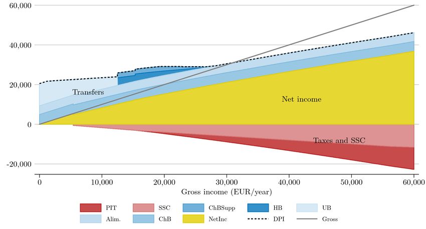
3.5 Visualization
The tax-benefit module can be used to visualize certain features of the German Tax-
Benefit System. Figure 2 decomposes the total disposable income (the dashed line
on top) of a hypothetical single household into benefits received, tax and contribution
payments, as well as net income for a given value of market income on the horizontal axis.
The decomposition is demonstrated for a single parent with two children in Figure 3.
Comparable figures for couples with and without kids are shown in Figures 9 and 10 in
the Appendix. It is assumed for the figures that adults are in the labor force and thus
eligible for unemployment benefit. Furthermore, full benefit take-up is assumed.
The figures demonstrate the basic unemployment benefit fading out as gross income
rises. It can also be seen that social security contributions form the major fraction of
the payment burden for households with gross income below A
C 50,000, as they kick in at
a fairly low income level. Figure 3 demonstrates the interaction between Unemployment
29
§1612a BGB and Mindestunterhaltsverordnung.
30
See § 26 SGB I and Wohngeldgesetz (WoGG).
14Note: The graph shows the development of the disposable income (DPI) applied to the gross in-
come (Gross) of a household after deduction of all components: Income tax (PIT), social security
contributions (SSC), housing benefit, unemployment benefit II as well as net income after the deduction
of the income tax and social security contributions (net). All information in EUR/year. Source: ifo
Microsimulation model.
Figure 2: Income components – Status quo (2020) – Single
Note: The graph shows the development of the disposable income (DPI) applied to the gross in-
come (Gross) of a household after deduction of all components: Income tax (PIT), social security contri-
butions (SSC), advance payment of maintenance/alimony (Alim.), child benefit supplement (ChBSupp),
housing benefit, unemployment benefit II as well as net income after the deduction of the income tax and
social security contributions (net). All information in EUR/year. Source: ifo Microsimulation model.
Figure 3: Income components – Status quo (2020) – Single parent, two children
15Note: The graph shows the effective total marginal burden from taxes, social security contributions
and transfer withdrawal for a given gross income of a household. Graphical truncation at 120 percent.
Source: ifo Microsimulation model.
Figure 4: Marginal burden – Status quo (2020) – Single
Benefit II, the Supplementary Child Benefit and Housing Benefit.31 If either of the
latter two is sufficient to raise household income above the subsistence level, they are
given priority to the unemployment benefit. As income increases, housing benefits and
supplementary child benefits fade out.
From a behavioral perspective, it is more interesting to analyze the pattern of the
effective marginal tax rate (EMTR). The EMTR is defined as the change in the tax
liability for a marginal change in gross income. Hence, it is a measure for the incentive
to increase income at the margin, e.g. via increasing labor supply. Figure 4 plots the
EMTR for a single household.32
Monthly earnings of A
C 100 are not charged against the unemployment benefit. Hence,
EMTR is zero up to A
C 1,200. Afterwards, 80% to 100% of earnings are deducted against
Unemployment Benefit II. The bump just above A
C 20,000 is caused by two parallel rules
to compute the solidarity surcharge, of which the more favorable one is applied. For
higher income levels, the EMTR for singles is mostly between 40 and 50 percent. The
two steps in the EMTR pattern are induced by the assessment ceilings for social security
contributions (see Table 2). These are also the reasons why marginal tax rates of top-
31
We assume an average rent for a three-person household among those receiving UB II as of 01/2020.
32
Note that these marginal rates can show spikes to ±∞. These spikes occur because the net income
changes stepwise at these points for a small increase in gross income, i.e. the net income as a function
of gross income is not continuous at that point. This does not necessary mean that the absolute
change in net income is big.
16income earners are slightly lower than for the middle class. Beyond, it should be noted
that, except for lump-sum deductions, we do not assume any tax-deductible items in
this calculation. Accounting for these may create a significant difference between gross
income and taxable income, thus lowering the effective burden of taxation. In addition,
capital income, which is taxed with a flat rate of only 25%, plays an increasing role for
high-income earners.
4 Behavioral labor supply module
The evaluation of policy reforms is divided into two steps. First, purely static calcula-
tions yield so-called morning-after or first-round effects, holding labor supply decisions
constant and ignoring behavioral responses. In a second step, we analyze potential
changes in the labor market outcomes due to the reform. Thereby, the analysis accounts
for the fact that policy reforms not only change net incomes and tax revenues but also
affect the incentives whether and how much to work. Many policy measures like the
Hartz reforms in Germany or the Earned Income Tax Credit (EITC) in the US are even
targeted at increasing the incentives for participation in the labor market and increas-
ing hours worked. Ignoring behavioral aspects of a policy reform thus yields only an
imperfect image of the likely effects of the reform.
Structural labor supply models have become the standard tool to evaluate such behav-
ioral responses. The idea is to estimate individual preferences under the observed status
quo and to predict behavioral responses under the new policy regime but assuming pref-
erences to be constant. Within this structural approach, there are several possibilities
to model labor supply. A major distinction can be made between the use of continuous
and discrete behavioral models. We briefly describe these two strengths of the literature
and proceed by describing the static discrete choice labor supply model implemented in
the ifo Microsimulation Model.33
4.1 Discrete vs. continuous labor supply modeling
The first empirical approaches in labor supply modeling relied on the derivation of
marginal utility with respect to hours of work. This technique follows directly from the
standard textbook neoclassical labor supply models and assumes that the household’s
utility is maximized over a continuous set of hours of work. This approach was intro-
duced by Hausman (see, e.g. Hausman, 1981) and is therefore also known as Hausman
approach. However, the classical model has some shortcomings. First, labor supply
responses are restricted to the intensive margin and neglect the participation decision,
which contradicts the empirical observation that labor supply is more responsive on the
extensive than on the intensive margin (Heckman, 1993). Second, it has proven quite
33
This section draws heavily from Löffler et al. (2014b) and Löffler (2013).
17cumbersome to employ this kind of model in the case of couple households or when the
budget set is non-convex, which is often the case given the complicated tax and benefit
systems in many countries and also in Germany. Third, the estimation of these models
requires rather restrictive a priori assumptions Bloemen and Kapteyn (see, e.g. 2008)
and MaCurdy et al. (1990, for details) and the estimated models are very sensitive to
the underlying wages (Eklof and Sacklen, 2000; Ericson and Flood, 1997).
For these reasons, it has become increasingly popular since the mid-1990s to model
labor supply as a choice between different jobs or types—known as discrete choice
approach. Pioneered by Aaberge et al. (1995), van Soest (1995) and Hoynes (1996),
this approach incorporates the labor supply decision in the context of a random utility
model. The model is estimated comparing different levels of utility instead of deriving
the marginal utility over the set of possible working hours. This allows incorporating
the full complexity of taxes and transfers without worrying about non-convexities, non-
monotonicity or corner solutions in the choice set. The same is true for couple households
and the joint labor supply decision of both partners, which can be modeled rather eas-
ily in the discrete choice context. In addition to these technical considerations, highly
regulated labor markets as in Germany are also better described as a choice between
different jobs or discrete working hours categories instead of a continuous decision on
hours worked. Furthermore, a richer stochastic specification in terms of unobserved wage
rates of non-workers and random preferences can be incorporated into a discrete choice
model.
For recent surveys of the empirical literature on labor supply models, see, for example,
Blundell and MaCurdy (1999), Bargain and Peichl (2013), Löffler et al. (2014b), Bargain
et al. (2014) or Aaberge and Colombino (2014).
4.2 Labor supply estimation
We follow recent developments in the literature and implement the behavioral labor
supply module in a discrete choice context. Following the standard procedure in the
literature, we assume that the household’s head and his partner jointly maximize a
unitary utility function in the arguments consumption and leisure of both partners.
Stated mathematically, household n opts for alternative i if this alternative is utility-
maximizing:
n o
f f f f
U Cni , Lm m m m
i , Li , Pni , ni = max U f wnj hj , wnj hj , In , T − hj , T − hj , Pnj , nj
j∈Jn
(2)
where the household chooses from jobs or job types j ∈ Jn (including non-participation in
f
the labor market with j = 0), Cnj denotes consumption levels, Lm
j and Lf denote leisure
of the male and the female partner, respectively, Pnj denotes whether the household is
eligible for and also claims welfare participation. The function f (·) represents the tax
18and transfer system that transforms gross to net incomes, In denotes non-labor income of
f
the household, T is the total time endowment, hm
j and hj denote working hours of both
spouses and nj captures unobservable tastes or disutility components for household n
when choosing job j.
In line with the common procedure in the literature, we assume that households choose
from a set of predefined job types, classified according to intervals of work hours. Single
decision-makers decide to work 0, 10, 20, 30, 40, 50, 60 hours per week, couples face
7 × 7 = 49 hours alternatives. This classification of intervals also roughly corresponds to
the observed hours’ distribution. Although this choice set representation is sometimes
criticized because of the arbitrary classification of working hours (see, e.g. Aaberge et
al., 2009), sensitivity analyses have shown that these rather typical hours intervals are a
good approximation to more flexible models (Bargain et al., 2014; Flood and Islam, 2005,
see, e.g.). Moreover, for every job type that makes the household eligible for transfer
receipt, households decide whether to claim the benefit. In principle, this makes up to
14 alternatives for singles and 98 alternatives for couples. However, welfare eligibility
often ends at the latest when working full-time.
4.2.1 Utility specification
As in the standard conditional logit model of McFadden (1974), we assume that un-
observables nj are additive separable and i.i.d. extreme value type I distributed. This
leaves us with the specification of the systematic part of the utility function. The ifo
Microsimulation Model incorporates a set of different utility specifications of which all
three are frequently used in the literature (see survey in Löffler et al., 2014b).
Quadratic utility specification The so-called quadratic utility function describes a
second-order polynomial in the choice variables consumption and leisure. This speci-
fication has been used, e.g. in Blundell et al. (2000a,b) and Bargain et al. (2014).
f 1 0 f
U q Cnj , Lm 2 m
j , Lj , Pnj , nj = xnj β1 Cnj + β2 Cnj + β3 Cnj Lj + β4 Cnj Lj
2 0 m 2 3 0 f f 2
+ xnj β5 Lj + β6 Lm
j + xnj β7 Lj + β8 Lj
4 0 5 0
+ xnj δ Pnj + xnj γ + nj (3)
In addition to consumption and leisure and their squared terms, the utility function also
accounts for potential stigma from welfare participation δ (if Pnj = 1) and labor market
restrictions such as fixed costs or working hours regulations γ.
Translog utility specification A slightly different version of the quadratic utility func-
tion is known as translog utility specification. In this form, the logs instead of the levels
of consumption and leisure enter the utility function. The translog specification has been
19used, e.g. by Haan (2006) and van Soest (1995) and Flood et al. (2007).
f 1 0 f
U t Cnj , Lm 2 m
j , Lj , Pnj , nj = xnj β1 ln Cnj + β2 (ln Cnj ) + β3 ln Cnj ln Lj + β4 ln Cnj ln Lj
2 0 3 0 f f 2
+ xnj β5 ln Lm m 2
j + β6 (ln Lj ) + xnj β7 ln Lj + β8 (ln Lj )
4 0 5 0
+ xnj δ Pnj + xnj γ + nj (4)
Again, the pure utility is given by coefficients β1 to β8 . The vector δ denotes the potential
disutility from welfare participation, γ captures labor market restrictions.
Box-Cox utility specification The third utility specification refers to a Box-Cox trans-
formed functional form. The Box-Cox specification has been used, e.g. by Aaberge et al.
(1995) and Blundell and Shephard (2011) and Löffler et al. (2014b).
f
(λ ) (λ ) m (λ ) (λfL )
U b Cnj , Lm 1 0
j , Lj , Pnj , nj = xnj β1 Cnj
C
+ β3 Cnj C Lm
j
(λL )
+ β4 Cnj C Lfj
2 0 m (λL ) m
3 0 f (λfL ) 4 0 5 0
+ xnj β5 Lj + xnj β7 Lj + xnj δ Pnj + xnj γ + nj
(5)
m (λfL ) (λ )
The Box-Cox variables Lm
j
(λL )
, Lfj and Cnj C are defined as follows (s = m, f ):
s
∗ λ s∗λ
Cnj C −1
if λC 6= 0 s
Lj sL −1
if λsL 6= 0
(λ )
Cnj C = λC
Lsj (λL ) = λL
(6)
ln C ∗
if λC = 0 ln Ls ∗
if λsL = 0
nj j
∗
Cnj = Cnj /1000 Lsj ∗ = Lsj /80 (7)
1 to x5 capture individual and household
In all these specifications, the vectors xnj nj
5 includes alternative specific variables as well. Thereby,
characteristics, the vector xnj
all three utility specifications allow for observed heterogeneity in preferences. In ad-
dition, it has become standard practice in structural labor supply models to allow for
unobserved heterogeneity in preferences as well. We incorporate this possibility in the
ifo Microsimulation Model by allowing preference coefficients (β1 to β8 , δ and γ) to
be random. This modeling approach—known as random coefficients model—assumes
that specific parameters are multivariate normally distributed.34 The rather technical
extension allows us to estimate the full distribution of tastes across all households in
our sample (more specifically, the mean and the variance of this distribution) instead of
estimating just the average preference for consumption or leisure.
As noted before, we not only model preferences for the level of consumption, but
also take account of the source of income by allowing for potential disutility δ from
34
We introduced unobserved heterogeneity in three coefficients, one in β1 , one in β5 and one in β7 .
20welfare participation (Moffitt, 1983). The underlying rationale is to pick up the empirical
observation that some households decide not to become welfare recipients although they
would be eligible. One reason might be that households do not want to enter the welfare
bureaucracy for a potentially small benefit payment. This modeling approach has been
proposed by Hoynes (1996) and Keane and Moffitt (1998).
Labor market regulations also crucially influence individual labor market decisions. In
the literature, different approaches have been taken. While van Soest (1995) arbitrarily
allowed part-time jobs to have lower utility levels, e.g. due to higher search costs, Euwals
and Soest (1999) introduced fixed costs of working instead of part-time restrictions.
Although fixed costs are easier to interpret, their modeling assumption remains rather
ad hoc. Aaberge et al. (1995) provide a theoretically more convincing concept that
models the share of market opportunities and peaks in the working hours distribution
due to working hours regulations. The behavioral labor supply module implemented in
the ifo Microsimulation Model incorporates all these different approaches.
4.2.2 Wage imputation
In order to evaluate the latent and thus unobserved choice set, we have to produce
counterfactual choice alternatives and calculate what the household’s consumption would
be, had it chosen a job type different from the observed one. A crucial issue when
estimating preferences and labor market conditions thus concerns the imputation of
hourly wages. Wage rates have to be imputed at least for non-workers, but some authors
also impute wages for the full sample of all households trying to avoid two distinct wage
distributions—the observed one for actual employees and the estimated one for non-
workers.
In addition to the imputation method, there are also different methods to predict
wages. The most important issue relates to the treatment of wage prediction errors.
Often, only the average predicted wage is used for the estimation, assuming that of-
fered jobs pay this wage with certainty. Instead of this rather restrictive assumption,
it becomes more and more common practice, to take account of the full distribution of
wage predictions and integrating the wage prediction error out during the labor supply
estimation.
Löffler et al. (2014b) show that the modeling decisions of how and for whom to impute
wages substantially impact the estimated labor supply elasticities. In fact, some impu-
tation methods lead to a substantial bias and even double the estimated labor supply
elasticities.
4.2.3 Estimation
To uncover the preference coefficients, we estimate the outlined model via maximum
likelihood methods. While the simplest version of this model reduces to a standard con-
21ditional or multinomial logit model with a closed-form solution, this model exhibits the
assumption of Independence of Irrelevant Alternatives (IIA, see, e.g. Luce, 1959). The
IIA assumption implies that the preference between two alternatives does not depend
on the presence or the characteristics of any other alternative. This assumption may
sometimes be justified but will rather be restrictive and unrealistic in most cases. There-
fore, it is common practice to also include unobservable components as in the random
coefficients model or prediction errors in wages. Both extensions depart from the sim-
ple multinomial logit model and thereby also yield more complex substitution patterns,
overcoming the IIA assumption.
In turn, these mixed logit models (McFadden and Train, 2000) no longer have a closed-
form solution. The reason is that the probabilities of household n choosing job type i
now have to be evaluated over the range of possible individual preference coefficients βn ,
labor market conditions γn and wage predictions ŵn :
N Z +∞ Z +∞ Z +∞
Y exp (vni {·|ŵni , βn }) g (i|γn )
L= f (βn , γn )f (ŵn ) dβn dγn dŵn
j∈Jn exp vnj ·|ŵnj , βn
P
n=1 −∞ −∞ −∞ g (j|γn )
(8)
By evaluating the full set of coefficients and wage predictions—each weighted by the
respective probability density—, we are able to estimate the distribution of the coeffi-
cients and not only population averages. In order to estimate this kind of model, Train
(2009) proposes the use of simulation methods to approximate the integrals of equation
(r) R
n o
(r) (r)
(8) and maximize a simulated log-likelihood based on a sequence βn , γn , ŵn
r=1
with r = 1, . . . , R draws sampled from the (joint) distributions of (βn , γn , ŵn ). The
maximum simulated log-likelihood is given by:
n o
(r) (r) (r)
N R exp vni · ŵni , βn g i γn
X 1 X
ln(SL) = ln . (9)
n o
R r=1 P (r) (r) (r)
n=1 j∈Jn exp vnj · ŵnj , βn g j γn
We use Halton sequences instead of (pseudo) random draws in order to increase the
stability of our estimation results. The labor supply estimation is performed using the
Stata command lslogit (see Löffler, 2013, for technical details on the estimation).
4.2.4 Benchmark model
While the ifo Microsimulation Model allows us to easily check the sensitivity of our results
with regard to the utility specification or the wage imputation procedure, our benchmark
model uses a setting that is both computationally feasible and able to replicate the
observed hours distribution. This is satisfied by a model that assumes a translog utility
function as in Equation 4. Preference coefficients are assumed to be non-random, and the
individual choice set is inflated to endogenize the welfare participation. Labor market
regulations are adopted according to Aaberge et al. (1995). We use predicted wages only
22You can also read