Heterogeneous Real Estate Agents and the Housing Cycle

∗
   Heterogeneous Real Estate Agents and the Housing Cycle

                                  Sonia Gilbukh†                 Paul Goldsmith-Pinkham‡

                                                       October 30, 2019

                                                             Abstract

           The real estate market is highly intermediated, with 90 percent of buyers and sellers hiring an agent to
       help them transact a house. However, low barriers to entry and fixed commission rates result in a market
       where inexperienced intermediaries have a large market share, especially following house price booms.
       Using rich micro-level data on 10.4 million listings, we first show that houses listed for sale by inexperienced
       real estate agents have a lower probability of selling, and this effect is strongest during the housing bust. We
       then study the aggregate implications of the distribution of agents’ experience on housing market liquidity
       by building a dynamic entry and exit model of real estate agents with aggregate shocks. Several policies
       that raise the barriers to entry for agents are considered: 1) lower commission rates, 2) increased entry
       costs, and 3) more informed clients. Relative to the baseline, all three policies lead to an increase in average
       liquidity, with the largest effect during the bust.

    ∗ First version: March 15, 2017. This version: October 30, 2019. We thank Luis Cabral, Stijn Van Nieuwerburgh, Petra Moser, David

Backus, and John Lazarev for their invaluable support and guidance. Gara Afonso, Edward Coulson, Diego Dariuch, Hanna Halaburda,
Andrew Haughwout, Julian Kozlowski, Virgiliu Midrigan, Brian Peterson, Pau Roldan, Thomas Sargent, and Lawrence White provided
helpful discussions and suggestions. We also greatly benefited from comments by Vadim Elenev, Jihye Jeon, Nic Kozeniauskas, David
Lucca, Joe Tracy, and Jacob Wallace. In addition, we thank seminar participants at NYU Stern in Macro and IO, the Federal Reserve Bank
of New York, the Federal Reserve Board, the Bank of Canada, Baruch College, London School of Economics, Harvard Business School,
Colorado Finance Summit, Pre-WFA Real Estate Meeting, Society of Economic Dynamics, AREUEA International conference, GBRUES,
Haverford, Hong Kong University, University of Toronto IO, and CREFR groups for valuable comments and suggestions. Sonia Gilbukh
gratefully acknowledges the hospitality of the New York Federal Reserve Bank of New York where she spent the summer of 2017. Part
of the work on this paper was completed while Goldsmith-Pinkham was employed by the Federal Reserve Bank of New York. The
views expressed are those of the authors and do not necessarily reflect those of the Federal Reserve Bank of New York or the Federal
Reserve Board.
    † Zicklin School of Business, Baruch College, The City University of New York. Email: sophia.gilbukh@gmail.com.
    ‡ Yale University, School of Management. Email: paulgp@gmail.com.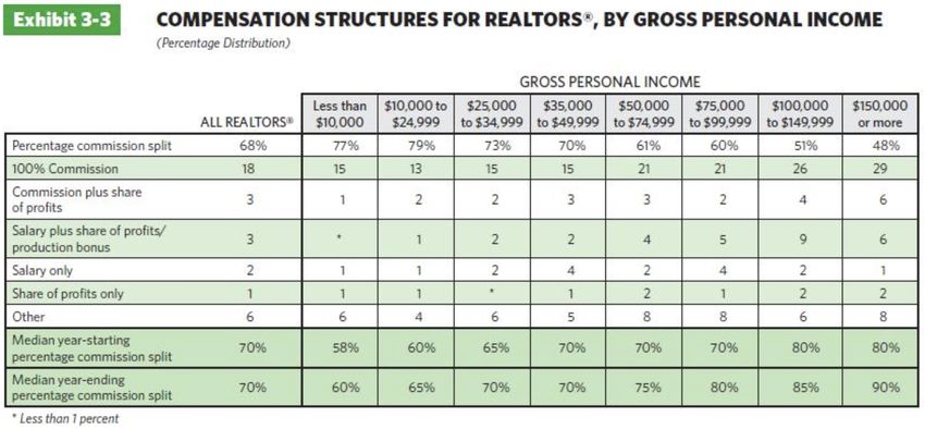

1     Introduction
The US housing market is subject to strong boom-bust cycles. The collapse prior to the Great Recession pro-

vides a particularly severe illustration: from 2006 to 2008, house prices dropped by 18 percent, while the proba-

bility of a house selling within a year of listing fell by 28 percent, from 67 percent in 2005 to 48 percent in 2008.1

Despite a large literature studying the significance of expectations, financial conditions, and other frictions in

generating and amplifying the housing cycle, few studies have focused on a prominent feature of this market:

real estate agents.2 Not only are agents central to the matching process between buyers and sellers—88 percent

of home buyers and 89 percent of home sellers use an agent (National Association of Relators, 2017)—but low

barriers to entry and fixed commission rates result in a market where inexperienced intermediaries have a

large market share, especially following house price booms.

      This paper studies how the experience of agents affects the sale probability of homes listed for sale and

how this effect aggregates to influence overall housing liquidity through the distribution of experience. Com-

bining micro-level empirical evidence and a dynamic model of entry and exit, we show that the presence of

inexperienced agents leads to reduced liquidity, with a larger impact in the downturns that follow housing

booms. Downturns are particularly affected for two reasons: first, not only are inexperienced agents worse

at selling listings but they are also especially bad during housing busts. Second, due to low barriers to entry,

the housing boom attracts many new agents into the profession, intensifying competition for clients and thus

hindering experience accumulation. These new agents remain in the market for the onset of the downturn,

resulting in a distribution skewed toward lower experience.

      We begin by documenting two empirical facts using a rich micro-level dataset of 10.4 million transactions

over the 2001–2014 period on 60 different Multiple Listing Service (MLS) platforms. First, an agent’s work

experience is highly predictive of how successfully and quickly they can sell homes. All else equal, listings

with agents in the 10th percentile of experience sell with a 11.3 percentage point (pp) lower probability than

those listed by agents in the 90th percentile. Second, this difference varies significantly over the housing cycle,

ranging from 8.2 pps in the boom to 13.2 pps in the bust. When compared to the respective average sale
    1 Source:authors’ calculations using the S&P/Case-Shiller US National Home Price Index and CoreLogic Multiple Listing Service
database.
   2 Favilukis, Ludvigson, and Van Nieuwerburgh (2017) illustrate the role of relaxing financial constraints on house prices. See Davis

and Van Nieuwerburgh (2015) and Guerrieri and Uhlig (2016) for literature review on financial frictions and the housing cycle. Among
many papers exploring search and information frictions in this market are Hong and Stein (1999), Head, Lloyd-Ellis, and Sun (2014),
Ngai and Tenreyro (2014), Anenberg (2016), and Guren (2018).

                                                                  1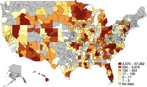

probability of 66.1 and 48.2 percent in those periods, the effects correspond to a 12.4 percent and 27.3 percent

advantage in liquidity.

     A key challenge in this empirical exercise is the lack of random assignment between listings and agents. As

a result, two types of selection bias could confound our results: selection on property (or listing) characteristics

and selection on listing client characteristics. For example, a more experienced agent might select to work with

easier-to-sell properties or more motivated clients. To address these selection channels, our estimates control

for a rich set of housing characteristics as well as zip-code-by-list-year-month fixed effects. We find similar

estimates in robustness results controlling for additional home and homeowner characteristics using historical

deed data as well as two subsample analyses where these selection effects are less likely to be a concern.

     We also show the consequences of the probability of sale beyond the initial listing. During the housing

bust, the ability to quickly sell a home was crucial for homeowners who had difficulty making their mortgage

payments. Those who fell delinquent on their mortgages and failed to sell were forced into foreclosure. Listed

homes that failed to sell in 2008 had a 5.5 percent chance of going into foreclosure in the next two years as

compared to close to 0 percent for sold properties. Highlighting the importance of experience in real estate

agents, we find that houses that listed in the bust years with inexperienced agents are 0.9 pps more likely

to subsequently foreclose (30 percent of the average probability of subsequent foreclosure during that period)

compared to those listed with experienced agents. Thus, not only did the inexperienced agents affect individual

sale outcomes, but they also contributed to negative externalities on the neighboring properties through the

foreclosure channel.3

     Our main empirical results focus on the overall effect that real estate agent experience has on the prob-

ability of sale but do not focus on the mechanisms that cause experience to increase the match probability.

One salient mechanism that sellers particularly care about is strategic pricing. Since properties with lower

list prices are more likely to sell, ceterus paribus, if experienced agents list properties with lower list prices

that will lead to higher listing liquidity. Using repeat sales data, we show that more experienced agents do

list properties for lower list prices, leading to slightly lower sale prices. However, the difference in markup on

a similar property is very small relative to the overall effect of experience on the probability of sale. Using a

back-of-the-envelope calculation, we estimate that the price channel makes up only about 20 percent of the

overall impact of experience on listing liquidity. Hence, we choose not to distinguish between mechanisms

affecting experience advantage and focus on the overall effect only.

     Assessing the potential improvement in aggregate housing liquidity through the real estate agent channel
   3 A body of papers have documented the externalities imposed by foreclosures on local housing markets, including Lin, Rosenblatt,

and Yao (2009), Campbell, Giglio, and Pathak (2011), Mian, Sufi, and Trebbi (2015), and Gupta (2016).

                                                                 2

is difficult because agent experience is endogenous. Agents’ choices to enter and exit, as well as their accu-

mulation of experience, depend on market conditions. Empirically, we show that entry and exit decisions are

affected by local house prices, volume of listings, and the market tightness. We consider policies that improve

liquidity by changing agents’ economic incentives to affect the distribution of experience. To accurately assess

the impact of these policies, we build a structural model that embeds housing search in a dynamic labor market

of real estate agents with aggregate market fluctuations.

    The model features frictional search in the housing market, where agent earnings depend on their expe-

rience. Experience has three advantages. First, agents with higher experience work with more clients. We

assume that some buyers and sellers look for an agent at random, while the rest seek a recommendation. This

implies that each agent is approached by a number of clients (sellers and buyers) that is an increasing function

of experience. Second, experienced agents have access to a more efficient matching technology for their seller

clients and thus have a higher probability of finding them a buyer and of earning a commission. Finally, the

model assumes that agents with higher experience get to keep a higher portion of their commission when

splitting it with the office where they work in. While we do not explicitly model offices, we assume that agents

only keep a fraction of their commissions.

    We then embed the matching market of housing into an entry and exit model of real estate agents with

aggregate market fluctuations. Our setup includes three aggregate states: bust, boom, and medium. Each state

corresponds to the number of sellers willing to sell their house as well as the valuation for houses by the buyers.

Agents’ decisions to participate as intermediaries depend on aggregate market conditions, competition they

face for clients, their success in earning commissions, and the value of accumulating experience and remaining

in the industry in the future years. These features generate empirically realistic fluctuations in the overall entry

and exit patterns of agents.

    Solving for an equilibrium of a heterogeneous agent model with aggregate fluctuations is challenging.

The distribution of agent experience depends on the entire history of aggregate state realizations and is a

pay-off-relevant variable on which real estate agents base exit and entry decisions. Keeping track of the full

distribution of experience effectively makes the state space infinite. To address this, we adopt an oblivious

equilibrium concept, introduced in Weintraub, Benkard, and Van Roy (2010). In this equilibrium, agents do not

perfectly observe the entire distribution of experience but instead approximate it by conditioning the experi-

ence distribution on the aggregate state in the current and previous period.

    Using this dynamic model calibrated to our empirical moments, we consider the impact of three counter-

factual policies: reducing commission rates, increasing entry costs, and informing clients of the importance of

                                                         3

experience. Relative to the baseline, doubling entry costs, halving commission rates, and decreasing the share

of uninformed clients who look for an agent at random all lead to a 3 percent increase in average liquidity,

with the largest effect of nearly 4 percent during the bust and a smaller 2 percent increase during the boom.

However, each policy acts through different channels.

     While the policies have comparable effects of aggregate liquidity, the three policies have different effects

on seller valuations and on the level of employment of real estate agents. Reduction in commission rates has

the largest positive effect on seller valuations, while decreasing the share of clients who look for an agent at

random has the smallest negative impact on the level of employment. Interestingly, doubling entry costs is less

effective along both margins but may be the policy that is most straightforward to implement, for example, by

raising licensing fees. This would also allow states to collect additional revenues and may be the most political

expedient.

     This paper contributes to a literature incorporating search frictions into understanding aggregate housing

market fluctuations (Head, Lloyd-Ellis, and Sun, 2014; Ngai and Tenreyro, 2014; Anenberg, 2016; Guren, 2018).

Our key contribution relative to this literature is to incorporate the heterogeneity in match technology due to

real estate agents’ differential experience. This builds upon a large literature, summarized in Han and Strange

(2015), which studies the role of real estate agents in search models.

     Our paper most closely relates to Barwick and Pathak (2015), who study similar data from the Greater

Boston area for years 1998–2007 and examine the effect of cheap entry on the probability of sale of listed

houses. An important distinction is that we model agent learning as an endogenous process, allowing for

differences in experience accumulation across aggregate states and for different overall competition levels.

By explicitly modeling this channel, we incorporate the learning externality that entering agents impose on

other intermediaries. In addition, our data cover 60 different markets across the US and extends through 2014,

allowing us to explore the recent housing bust in a setting that is not specific to one area. Hsieh and Moretti

(2003) and Han and Hong (2011) also study the effect of cheap entry on market efficiency, specifically focusing

on the business-stealing externality and abstracting from experience all together.

     More broadly, this paper contributes to a large literature on the value of real estate agents. Hendel, Nevo,

and Ortalo-Magné (2009) compare listing outcomes from an FSBO (for sale by owner) platform to those who

were facilitated by an agent. They find that agents provide little value added. Levitt and Syverson (2008) find

that agents can obtain a better price when they are selling their own homes rather than those of their clients.

These papers abstract from agent heterogeneity, which we argue can have a significant impact on value added

for a client.

                                                        4

The rest of the paper is structured as follows. Section 2 describes industry background. Section 3 describes

data and our choice of measure of experience. In Section 4, we present the empirical analysis. Section 5 outlines

the model and the calibration exercise. Section 6 presents results from the counterfactual analysis. We conclude

in Section 7.

2     Real Estate Agents in the United States
Despite the existence of numerous FSBO platforms, the housing market in the US remains highly intermediated,

with 87 percent of buyers and 89 percent of sellers hiring an agent to facilitate buying or selling a home

(National Association of Relators, 2017). There are many reasons why consumers find agents valuable. First,

an agent has access to the local MLS database, which provides detailed information on all the listings currently

available in the area and allows sellers to advertise to potential buyers.4 Second, an agent plays an invaluable

role as an adviser. For example, a listing agent suggests improvements, or “staging,” to make the property

more attractive to buyers, provides input on an appropriate listing price, and advises on whether to accept the

incoming offers. Last, an agent gives a client representation in a negotiation process in the final stages of the

transaction, making an agreement with the counterparty more likely. Through these three channels, hiring an

agent gives access to a more efficient matching technology between home buyers and sellers. Thus, a listing

agent not only attracts more buyers to the listing but also makes buyers more likely to bid on the property and

facilitates the transaction once a buyer is found.

      Despite the role of agents in facilitating one of the most important financial transactions in their clients’

lives, one can become a licensed real estate agent after only 30 hours of classes and a $50 exam fee.5 While these

classes familiarize agents with essential terminology and state laws, they provide little insight into local real

estate markets or into the most effective ways to create transactions. Hence, agents have a substantial room

for improvement after entry. In addition to learning about the local housing market and the tacit knowledge

of selling, agents accrue an accumulated network of former clients, other agents, and a long list of useful pro-

fessionals, such as construction workers, plumbers, electricians, mortgage brokers, appraisers, photographers,

and interior designers. Tapping into these networks makes a sale more likely by increasing the number of

potential counterparties for their clients and by ensuring that the property is “fixed up” and is more desirable

for a buyer. Hence, the inexperience of brand-new agents will likely make them worse at getting properties

sold when compared to incumbent experienced agents. This is a key empirical issue that we assess in Section
    4 The creation of web platforms such as Zillow and RedFin has reduced agents’ monopoly over the information on available listings,

but agents maintain the exclusive ability to list on the MLS to advertise for-sale properties to other agents.
   5 The requirements vary somewhat across states, with class time ranging from 30–50 hours.

                                                                    5

4.

     While there are potentially large differences in the experience of agents, the compensation paid by buyers

and sellers to real estate agents does not appear to vary across agents. As highlighted in other work studying

agents, commissions in the market appear to be relatively fixed across agents, regardless of agent quality (Hsieh

and Moretti, 2003; Barwick and Pathak, 2015; Barwick, Pathak, and Wong, 2017; Barwick and Wong, 2019). The

ease of entry and fixed pricing results in many agents entering the industry for short periods of time.

     Despite being paid the same commissions as experienced agents, inexperienced agents appear able to

attract clients. In 2017, the National Association of Realtors (NAR) found that 74 percent of sellers and 70

percent of buyers signed a contract with the first agent they interviewed (National Association of Relators,

2017). While the first agent contacted is likely not chosen at random, the survey indicates that clients do not

approach the choice decision with much care. One reason may be that clients do not realize the importance

of choosing the right agent or find it difficult to gauge experience. Alternatively, with so many people in

the profession, many clients personally know someone who is a licensed agent and hire them to avoid social

consequences. As a result, as we show below in Section 3, these inexperienced agents have a non-negligible

share of the market.

     It is not just clients who are affected by the prevalence of new and inexperienced agents. The industry has

raised alarms about this phenomenon. In 2015, real estate agents identified the number one challenge to their

industry to be “Masses of Marginal Agents Destroy Reputation” in a report commissioned by the NAR: “[t]he

real estate industry is saddled with a large number of part-time, untrained, unethical, and/or incompetent

agents. This knowledge gap threatens the credibility of the industry.” In another report commissioned by

Inman, an industry periodical, 77 percent of agents responded “low-quality agents” to the question “what are

the challenges that the real estate industry is currently facing?”6

     There are three channels through which agents might be affected by the widespread presence of inexpe-

rienced competitors. First, the inexperienced competitors may be less effective at matching their clients, thus

lowering the average expectation of potential home buyers and sellers of the value of intermediaries. This can

discourage clients from entering the market. Second, as described in Hsieh and Moretti (2003), the ease of entry

results in an excessive amount of real estate agents in the industry, which results in any one agent working

with fewer clients, thus lowering their total profits. Finally, with the intensified competition, agents focus a
    6 A relevant respondent quote in the Inman report: “A great many agents are part-time. Other than the few transactions they

finagle out of their family/ friends yearly they have very little to do with the industry and don’t care to educate themselves or increase
their skills. This is a disservice to their clients and gives real estate professionals a bad name.” For more information about the
Danger Report commissioned by the NAR, see their website: https://www.dangerreport.com/usa/. The Inman report is available here:
https://www.inman.com/2015/08/13/special-report-why-and-how-real-estate-needs-to-clean-house/.

                                                                    6

large amount of their time attracting clients rather than directly working with buyers and sellers. As a result,

they cannot accumulate the relevant experience to become better at matching their clients. This is a second

form of “crowding” out: in addition to social waste from agents spending resources to take business from one

another, as described in Hsieh and Moretti (2003), agents also take from each other the ability to improve their

matching technology by accumulating experience.

3     Data and Measurement
In this section, we describe our data sources and the various sample restrictions that we use. We then discuss

how we measure real estate agent experience and summarize our measure.

3.1    Data Sources

For our main empirical analysis, we use a comprehensive listing-level dataset on residential properties for sale

collected by CoreLogic. The data come from MLS platforms operated by regional real estate boards. Each MLS

varies in size but, on average, covers a geographical area that is approximately equal to a commuting zone. Each

observation in the data represents a listing on an MLS platform, with a large number of variables describing

the property and the status of the listing. These include the date the property is listed, the associated listing

agent (as well as secondary agent in some cases), the original list price, the last observed list price, and detailed

property characteristics such as the living area, number of bedrooms and bathrooms, number of parking spaces,

and age of the structure. If the listing sells, we observe the date of sale, the sale price, and the associated buyer

agent. If the property fails to sell, we also observe when the property is pulled from the market. Crucial for

our analysis is that each real estate agent in an MLS is given a unique identifier such that we can track them

throughout the sample.

      The full CoreLogic MLS dataset has information on over 150 MLS platforms. However, the history for

each MLS in this dataset begins at different times due to variation in CoreLogic’s contracts with each MLS,

with some data beginning as late as 2009. Since we are interested in studying the boom period starting in 2001,

we restrict our analysis to the subsample of MLS whose data begin in 2001. Additionally, due to data quality

issues, we drop several MLS whose data begins in 2001 or earlier but have large jumps in the number of listings

during the sample period from 2001–2014 (more than 100 percent growth in the number of listings in a given

year). This final restriction drops an additional 10 MLS and leaves 60 MLS platforms in our sample. Within

these MLS, we exclude listings with asking prices below $1,000. This leaves us with 10.4 million observations.

Appendix Figure H1 shows the coverage map of the final sample. A key feature of our dataset is that while we

do not have full coverage of the United States, we have near-exhaustive coverage within a geographic location,

                                                         7

ensuring that we observe all potential transactions by real estate agents in an area. Over the sample period

from 2001 to 2013, we observe 569,148 different agents, with an average of 175,458 active agents in each year.

      In addition to the MLS data, our robustness analysis makes use of two additional datasets. First, we use

proprietary deed-level data purchased from CoreLogic, which contain information on housing transactions and

their associated transaction prices recorded at county deeds offices. Using this data allows us to supplement

our analysis in two ways: first, we identify properties that subsequently fall into foreclosure. Second, we

identify the price that a listing was previously transacted at, which gives us a way to control for unobserved

heterogeneity of properties.

      Our second dataset is Zillow’s publicly available zip-code-level house price index. We use this time series

to construct a measure of “inferred price” for listings of previously transacted properties. To do so, we take the

listed properties’ previously transacted price and use the realized house price appreciation in the listing’s zip

code to identify the approximate market price for the listing.

3.2    Measurement of Experience

We next describe how we measure real estate agent experience. Ideally, our measure captures three features of

real estate agent activity. First, our measure should be consistent over the sample period. Thus, a backward-

looking measure, such as time spent as a real estate agent, will be inaccurate because our information about

agents’ history is censored in 2001 at the beginning of sample. Second, our measure should be consistent

over locations. Hence, using an income-based measure will inaccurately assign higher experience to agents

who work in high price areas. Third, the measure should capture as many sources of potential experience as

possible.

      Our preferred measure is the number of clients an agent had in the previous calendar year, as it closely

matches those requirements. This measure captures three types of transactions: the number of listings sold

by the agent in the previous year, the number of listings unsold by the agent in the previous year, and the

number of buyers represented by this agent in a transaction that closed in the previous year.7 Thus, our

measure of experience is in terms of recent output, rather than calendar time since entry, and has a high

discount rate so that any clients who were served two or more years prior do not count toward the current

experience. This provides a consistent measure that can be calculated across all time periods, except 2001, in

our sample. Moreover, our measure assumes that all clients contribute to the experience level equally, no matter

the outcome of the listing, so that both unsold and sold properties count toward the listing agent experience.

This helps ensure that markets with higher and lower levels of sales and prices will be counted equally and
  7 We   are unable to measure clients with buyers agents who do not buy.

                                                                 8

also exploits all transactions that we observe in the data.

      In Appendix B, we discuss alternative measures and approaches to measuring experience, such as weight-

ing listings differently depending on sale outcome, discounting older listing differently, or using years since

entry for agents where we observe entrance. We find that these alternative measures do not materially affect

our results but either limit our sample (due to the longer required time period) or do not map to our theoretical

measure of experience.

      In Figure 1(A), we plot the distribution of experience of active agents, pooling across all years in our

sample. Notably, almost 30 percent of all agents are completely inexperienced, with no previous clients. In

Figure 1(B), we again plot the distribution of experience, this time weighted by the agents’ active listings in

that year. While inexperienced agents now have less listings, compared to their unweighted presence in the

market, they still hold considerable market share. Twenty-five percent of listings are handled by agents who

had 4 or less clients in the past year, and 50 percent are listed with agents with an experience of 12 clients or

less. In other words, the majority of sellers used a listing agent who worked with one client a month (or less)

in the past year. Hence, if experience matters for liquidity, the prevalence of inexperienced agents could have

large aggregate effects in the housing market.

4     Empirical Results
In this section, we use our measure of experience to show a strong link between real estate agent experi-

ence and listing liquidity that varies over the housing cycle. We then highlight how the effect of experience

on liquidity affected foreclosures during the housing bust of 2008–2010. Finally, we discuss the challenge of

counterfactually changing agent experience. We show how agent experience itself varies over the cycle and

responds endogenously to market conditions, demonstrating the need for a structural model that accounts for

agents’ endogenous acquisition of experience.

4.1    Estimation Approach

We first estimate the effect of agent experience on listing outcomes. The challenge for this exercise is lack of

random assignment between listings and agents. Two types of selection can confound our results: selection

on property (or listing) characteristics and selection on listing client characteristics. For example, a more

experienced agent might select to work with easy-to-sell properties or with more motivated clients. To address

these selection channels, we present robustness tests using a rich set of housing and homeowner characteristics

and subsample analyses where these selection effects are less likely to be a concern.

      To examine the effect of agent experience on listing outcomes, we estimate versions of the following

                                                        9

regression:
                                              X
                           yi,t = αi,t +                βp log(1 + experiencei,t ) + δWi,t + i,t ,                             (1)
                                            p∈periods

where yi,t is the outcome for listing i in time t, experiencei,t is the experience of the listing agent for listing

i in time t, Wi,t is a vector of property-specific controls such as square footage and number of bedrooms,

and αi,t denotes time and location fixed effects based on the listing’s location. For most outcomes, time t

indicates the year-month of the listing, except for sale outcomes, where time t denotes the year-month of the

sale. To account for the highly skewed distribution of experience, we use log of one plus experience as our

main explanatory variable. In all regressions, unless noted otherwise, errors are clustered at the MLS level

to account for within-MLS correlation between our experience measure and unobservable shocks (Bertrand,

Duflo, and Mullainathan, 2004; Abadie et al., 2017).

      In our estimation, we allow the effect of experience to vary by time period. We do this in two ways. First,

for some of our graphical results, we allow the effect of experience to vary year-by-year and then plot the

effect for each year. Second, in anticipation of the calibration of our model in Section 5, we define three time

periods—boom, medium, and bust—which reflect the aggregate state of the housing market in each year. The

assignment of each year to period is based on 12-month real house price growth, as measured from 1960 to

2017 by the Case-Shiller index, deflated by the Consumer Price Index less costs of shelter. Years with growth

rates above the 75th percentile are identified as booms, those below the 25th percentile are busts, and those in

between are assigned to a medium period. Appendix Figure H2 illustrates this assignment procedure.8 In our

main tabular results, we report estimates pooled into each of the three time periods.

4.2    Effect of Experience on Listing Liquidity

We begin by focusing on the effect of experience on the probability of sale within 365 days of listing. In Figure

2, we present visual evidence of the strong positive relationship between listing liquidity and agent experience.

The slope in this plot corresponds to the β coefficient of Equation 1, controlling for zip-code-by-list-year-month

fixed effects. This figure does not allow β to vary by time period and so plots the pooled effect of experience on

sale probability over the full sample. The relationship is strikingly linear. The probability of sale within a year

for listings whose agents were in the 10th percentile of the experience distribution is almost 11.5 pps less when

compared to agents in the 90th percentile. More generally, doubling the experience of an agent corresponds to

approximately a 3.9 pp increase in the probability of sale.

      In Figure 3, we let the effect of experience vary by listing year, using the same set of zip-code-by-list-year-
   8 Years 2007, 2008, 2009, 2010, and 2011 are assigned to the bust period; years 2006 and 2012 are in the medium period; and years

2002, 2003, 2004, 2005, and 2013 correspond to the boom period.

                                                                10

month fixed effects as in Figure 2, and plot the corresponding βs with 95 percent confidence intervals. In this

plot, we see large changes in the effect of experience on listing liquidity, with an initial smallest effect of 0.033

(standard error (se) = 0.003) in 2004, the largest coefficient of 0.054 (se = 0.003) in 2009, falling again to 0.030

(se = 0.003) in 2013.

     We formally present estimates results from Equation 1 in Table 1. In each column, we report the effect

of experience on the probability of a listing’s sale within 365 days. In Column 1, we report the overall pooled

effect of experience, while in Columns 2–6, we allow the effect to vary based on the housing cycle, where the

base period is the housing boom. We have two sets of analyses: our main sample in Columns 1–3 in Panel A,

where we use all observations, and our repeat sale sample in Columns 4–6 in Panel B, where we use the sample

of listings that can be linked to the previous transaction of the property. The additional information from this

repeat sample lets us control for unobserved quality of the home and for confounding selection issues.

     We first focus on the full sample in Panel A. In Column 1, we report the overall pooled effect of experience

with zip-code-by-list-year-month fixed effects, corresponding to the estimated effect from Figure 2. In Column

2, we repeat the same exercise but allow the effect to vary by our three aggregate time periods, with the

base period of the housing boom. In Column 3, we add the following housing controls to capture property-

level characteristics: number of bedrooms, bathrooms, garages, living area, and type of cooling system and

indicators for waterfront property, view, and fireplaces.9

     Overall, there is a strong positive effect of experience on listing liquidity. Split out by time period in

Column 2, the effect is 3.2 pps during the boom periods, 3.6 pps in the medium house price growth periods, and

4.6 pps during the housing bust periods. After adding housing controls in Column 3, our preferred specification,

the effect shrinks slightly. Doubling the listing agent’s experience increases the probability of sale by 2.8 pps

(se of 0.3 pp) during the boom period. During the medium house price period, this effect grows to 3.4 pps.

Finally, doubling the listing agent’s experience in the bust has a 1.3 pp larger effect (se of 0.2 pp) than in boom

times, an increase of 46 percent, with an overall effect of 4.5 pps.

     To put these measures in terms of the overall distribution of experience, listings of an agent in the 90th

percentile (corresponding to an experience measure of 18) sell with a 8.2 pp higher probability than listings of

agents in the 10th percentile (corresponding to an experience of 0) during the boom period. In the bust period,

this gap increased to 13.2 pps. Compared to the average probability of sale of 63 percent during the boom

period and 47 percent during the bust, this implies an increase of 13 percent of the mean during the boom and

25.7 of the mean during the bust. Thus, not only is agent experience an important factor in whether a listing
    9 For each discrete characteristic, we dummy out the values to nonparametrically control for their effect. We censor the top 1 percent

of values in our controls to account for outliers.

                                                                   11

sells, but the importance grows as the housing market contracts, with the smallest effect of experience in the

boom and largest effect during the bust.

    In Panel B of Table 1, we exploit the panel nature of our transaction dataset to run two additional robustness

tests addressing potential selection issues. First, in Column 4, we rerun our preferred specification from Column

3 of Panel A, which uses zip-code-by-year-month fixed effects and housing controls but is restricted to the

repeat transaction sample as in Columns 4–6. Our restricted sample’s size is roughly one-third of the original

sample and is tilted toward later years in our sample.

    In our first robustness test, we consider the alternative mechanism that agents with higher experience

choose to work with properties that look observably similar (based on housing controls, location, and timing

of the listing) but have unobserved qualities that make them higher value. As a result, these properties might

be easier to sell. To address this issue, in Column 5, we control for the inferred price of each home. We measure

this using the previous observed sale price (as measured using deeds data) for the property and appreciating

the value of the home using Zillow zip-code- and tier-level house price appreciation indexes.

    We then consider the alternative mechanism that agents with higher experience choose to work with

clients who are easier to work with. To test this in Column 6, we control for the client equity at the time of

the listing, as proxied by the amount of house price appreciation experienced by the seller since the house was

last transacted. As argued in Guren (2018), there are two reasons why clients with lower equity are likely to be

less flexible in the selling process. First, low equity sellers are likely to be cash constrained, especially if they

are looking into purchasing another property and need money for down payment. Second, sellers who have a

higher equity in the property are less likely to experience loss aversion from selling at a lower price than what

they initially paid. Thus, controlling for equity allows for the alternative mechanism that agents with higher

experience choose to work with properties that look observably similar (based on housing controls, location,

and timing of the listing) but choose clients with higher amounts of house price appreciation and thus are more

flexible in the selling process.

    In Column 4, with the same controls in the repeat sample as our preferred specification, we find qualitia-

tively similar results. The effect of experience during the housing boom is large and statistically significant,

with a doubling of experience leading to a 3.9 pp increase in the probability of a listing sale. However, for

this subsample, there is a statistically insignificant difference between the boom period and the medium house

price growth period, likely due to the sample being tilted toward the later part of the sample (and limited ob-

servations during the medium period). There is still a large and significant difference between the effect of

experience in boom and bust periods, with the effect of experience increasing by 36 percent during the bust

                                                         12

period.

     In Column 5, controlling for a direct measure of inferred price, our estimates of the effect of listing agent

experience on sale probability are identical to Column 4. A similar result holds in Column 6 when controlling

directly for client equity. All effects are similar in size and magnitude across the cycle, while the R2 does

appreciably increase across specifications, suggesting that any selection by more experienced real estate agents

into houses is not driving the positive correlation between experience and sale probability (Oster, 2019).10

Additional Robustness Results In the Appendix, we provide two additional robustness tests to ensure

that our estimates are capturing the effect of experience on listing liquidity rather than capturing a selection

of experienced agents into easier-to-sell homes or more motivated sellers. First, in Appendix F, we restrict

our analysis to a homogeneous suburb of San Diego where all houses are nearly identical. In this market, the

standard deviation of prices for listings is less than 20 percent, and as a result, there should be limited selection

on houses by agents of differing experience. In Appendix Figure F2, we repeat the same approach as Figure 2

and find the same linear and monotonic relationship between agent experience and the probability of sale. In

Column 1 of Appendix Table F1, using our preferred regression specification from Column 3 of Table 1, we find

that the effect of experience on the probability of listing sale is still positive but is smaller in magnitude during

the boom period. However, the effect of experience in the medium and bust periods are large and significant,

similar to what we find in Table 1.

     As a second robustness check for selection on clients, we examine a subsample of listings that followed a

deed transfer that we assume proxies for a life-changing event (Kurlat and Stroebel, 2015). Specifically, we look

at listings that occur within two years of a previous transaction where both parties have the same last name but

have a different first name. These transactions likely capture a transfer of property from a married couple to

one partner, which likely happens in a case of divorce or death of one of the spouses. Sellers in this sample are

likely more motivated in getting rid of the property than an average seller because they either cannot afford

maintaining it or do not have use for it altogether. Using this sample, we repeat the same approach as Figure

2 in Appendix Figure H3 and find a similarly significant and linear effect of experience on sale probability.

Due to a smaller sample size across locations, we are unable to control for zip-code-by-list-year-month fixed
   10 Under the assumption of equal selection (δ = 1) and a maximum R2 of 1, the formal Oster (2019) selection bias adjustment would

be an upward adjustment of 0.019, suggesting that there is actually negative selection by experienced agents into more difficult-to-
sell listings. Formally, the Oster (2019) estimate of selection bias considers two components: the change in coefficient when adding
controls and the change in R2 . Since this test is defined for single treatment variables, we reestimate the regressions from Table 1
without time period interactions and consider the sample from Panel B. Our estimate and R2 in the full regression, Column 6 without
time interactions, are 0.046 and 0.2439. In the short regression, with just our experience measure, the estimates and R2 are 0.041 and
0.0147. In the Panel A sample, without the equity stake control, our estimate would have an upward adjustment of 0.027.

                                                                 13

effects and instead include county-by-list-year-month fixed effects. In Column 1 of Appendix Table I7, we

repeat our preferred specification for sale probability. We find a significant and positive effect of experience,

with a similar magnitude to Column 3 of Table 1. However, we do not find significant differences in the effect

of experience across boom and bust periods. Both robustness results suggest that our estimates are capturing

the effect of experience on listing liquidity rather than capturing a selection of experienced agents into listings

with easier-to-sell homes or more motivated sellers.

Additional Liquidity Measures While probability of sale in the next year is our preferred measure of

listing liquidity, there are many other potential proxies we could use in our data.11 In Appendix Tables I1 and

I2, we examine two alternative proxies: number of days that the listing is on the market and number of days

until sale. The first measure counts the number of days until a listing was either sold or withdrawn from the

market (a “failed” attempt to sell). The second measure counts the number of days until a listing is sold, which

excludes nonsales. In both cases, the faster a property sells, the more liquid it is. However, the latter outcome

conditions on sale, thus removing the extensive margin of liquidity. For both sets of analyses, we repeat the

same specifications as in Table 1 in Columns 1–6 using the full sample in Panel A and the repeat sample in

Panel B.

     In Appendix Table I1, we examine the effect of experience on a listing’s days on market. In Column 1 of

Panel A, we see that doubling an agent’s experience reduces the average days on market by approximately 4.9

days. Splitting the effects out by time period in Column 2, we find that this effect is smallest in boom periods,

with a doubling of experience leading to a reduction of 2.9 days on market, or 2 percent of the average listing

time of 137 days during the boom. This effect is larger in magnitude in medium house price growth periods

and largest during busts, where a doubling in experience leads to a reduction in over 7 days, or 3.9 percent of

the average listing time of 179 days on market during the bust. These effects are even larger once we control

for housing characteristics in Column 3 of Panel A, our preferred specification. In Panel B, using the repeat

sample, we find nearly identical estimates to Column 3 in Columns 4–6, ruling out selection on unobservable

property or client characteristics.

     In Appendix Table I2, we examine the effect of experience on a listing’s days to sale. Importantly, this

conditions on the subsample of listings that sell. As a result, this estimate is harder to interpret, as it conditions

on the extensive margin effect of experience on sale. In Column 1 of Appendix Table I2, we estimate that

doubling an agent’s experience leads to a reduction of 2.9 days to sale. In Column 2, we see again that this
  11 This   is similar to the bond market, where there are many potential proxies for liquidity (Houweling, Mentink, and Vorst, 2005).

                                                                   14

effect is smallest during the boom, reducing days to sale by 1.6 days (1.4 percent of the average days to sale of

116 days) and is largest during the bust, reducing it by 4.6 days (3.2 percent of the average days to sale of 143

days). The effects are similar when conditioning on housing characteristics and when using the repeat sample

in Panel B, again showing that the results are not driven by unobservable property or client characteristics.

      Both sets of results in Appendix Table I1 and I2 are consistent with agent experience increasing listing

liquidity. Experience has both a large effect on whether a listing sells at all as well as on the speed that a

transaction is sold within the year. We prefer the sale outcome within a year as a measure that captures both

the extensive and intensive margin of listing liquidity.

4.3    Agent Experience and Listing Prices

Our results so far have focused on the overall effect that real estate agent experience has on probability of

sale but not on the mechanisms by which experience increases the match probability. There are many ways

in which an experienced agent could improve the chances of a listing selling. For example, agents with more

experience are more connected to other agents and also former clients. Thus, they can attract more matches

for a listing by reaching out to potential buyers or by contacting other agents and tapping into their network

of clients. Moreover, a more experienced agent can more effectively market a property to attract viewings and

increase desirability for buyers who view the house. Finally, experienced agents might set lower list prices for

their properties, both attracting more clients and making the purchase more likely. While the client will benefit

from their agent’s network and expertise in the selling process, the client faces an important trade-off when it

comes to the property price. Since properties with lower list prices are more likely to sell, ceterus paribus, if

experienced agents list properties with lower list prices, then that will lead to higher listing liquidity.

      In this section, we explore whether agent’s choice of list price drives the liquidity advantage of experience.

In Table 2, using the preferred empirical specification from Column 3 of Table 1, we consider the impact of real

estate agent experience on several listing price measures. In all cases, we consider log outcomes. In Column 1,

we examine differences in list prices. We find that that a doubling of real estate agent experience is associated

with approximately a 1.3 percent decline in list prices during boom periods and a 3 percent decline during

busts. In Column 2, we see that these declines in list prices correspond to a similar decline in sale prices.

During boom periods, a doubling of experience corresponds to a 1.2 percent decline in sale prices and in busts,

a 2.5 percent decline. Note that this sale price is conditional on a successful sale. In Column 3, we show formally

that experience has no effect on the “discount” taken off of list prices, by estimating the effect of experience

on the ratio of list price to sale price. In all three periods, there is no significant difference, suggesting that the

subsequent sale price, anchored on the list price, is similar.

                                                          15

We next show evidence that this difference in list prices does not reflect unobserved quality of the property.

In Column 4 of Table 2, we use the inferred price of the home as the outcome variable. Recall that this measure

takes the last previously transacted price for this home and uses local house price indices to approximate the

value of the home at the listing date. As a result, we can see whether experienced agents work with homes

that are worth less, driving the negative price effect. During the boom period, a doubling of agent experience

is associated with a statistically insignificant 0.5 percent decline in inferred prices. During the medium house

price growth periods, this effect is also statistically insignificant. However, in the bust, that decline is 1.2

percent and statistically different from zero (se of 0.039). This suggests that only during bust periods do more

experienced agents select into slightly lower value homes. Thus the lower list prices are driven mainly by

agent and seller choice of listing price rather than the selection on homes.

     Finally, in Column 5 of Table 2, we examine by how much the experience reduces the listing price relative

to the inferred value of the home. We do so using the list price scaled by the inferred price from Column 4,

which is effectively the list price markup over our inferred price measure (this is a simple version of the markup

generated in (Guren, 2018)). A smaller ratio suggests a lower list price relative to the value of the home. We

find that across all time periods, a doubling of agents’ experience leads to a 1.5 pp decline in the relative list

price. Hence, the mechanism of agent experience acting through list prices does play a role.

     How much of this decline in list prices explains the effect of experience on listing liquidity? In Figure 4,

we plot a binned scatter plot of the probability of sale in 365 days against the list price, scaled by the inferred

value of the home, controlling for zip-code-by-list-year-month fixed effects and our housing controls. We plot

two relationships on this plot. First, in solid black triangles, we plot the overall relationship for all agents. As

expected, this relationship is strongly negative, with a decline from 1.1 pp to 0.9 pp in the normalized list price

leading to an increase in sale probability of roughly 10 pp.12 The effect of doubling experience on markups is

a reduction of 1.5 percent, suggesting that the effect of list price differences would lead to an increase in the

probability of sale by about 0.75 percent. Since the effect of experience on sale probability is roughly 3.9 pp

during the boom and 5.3 pp during the bust in Column 4 of Table 1, this implies that the listing price effect is

only a small share of the overall impact of experience on listing liquidity.

     We then split this figure by agent experience terciles (weighted by listing) and show that there is a stark

level difference in the probability of sale across experience levels, holding fixed the value of the list price

markup. While for all experience levels, a lower list price corresponds to a higher probability of sale, there

is a additive shift in the probability of sale for different experience levels, implying a large experience effect
 12 Our version of this relationship is much more monotonic compared to the ordinary least squares (OLS) figures in Guren (2018).

We discuss the difference in Appendix G.

                                                               16

independent of prices.13

      Using a back-of-the-envelope calculation, the price channel of experience makes up only about 20 percent

of the overall impact of experience on listing liquidity. This back-of-the-envelope calculation suggests that

listing prices, while important, play a limited role in the effect of agent experience on listing liquidity.14 Thus,

for the rest of the paper and in the model, we abstract from differing pricing strategies and focus on the overall

effect of experience on liquidity.

4.4    Foreclosure Consequences of Illiquidity

We have shown that real estate agent experience significantly affects the probability of sale. Why does the

ability to sell a home matter? First, many people change homes to accommodate the size of their household

and to be closer to a job, friends, or family. Inability to sell the current house thus impedes the purchase of a

home that better serves their needs. This channel is valuable across all time periods. Second, listing liquidity

can be important in the ability to reallocate financial resources from housing to more pressing needs, which

can be particularly valuable during a recession. During the recent housing crisis, many households found

themselves with expensive mortgages that they could not refinance due to tightening credit. Many attempted

to sell their properties but could not do so, and some were forced into foreclosure.

      Foreclosures result in a significant financial burden for people who lose their homes. A likely outcome

is a substantially lower credit score that limits borrowing ability for years to come. Foreclosures are also

socially inefficient because vacant properties tend to depreciate faster, either due to lack of upkeep or through

a higher chance of looting and crime, which reduces the value of the property and puts downward pressure

on prices for all houses in the neighboring areas. Several studies have documented that foreclosed properties

have externalities. This was particularly important in the recent bust, as lower prices might have caused more

homeowners to go into foreclosure.15

      In our listings data, we observe properties that enter foreclosure after being listed for sale as non-foreclosure

or non-REO properties. We focus on the outcome of whether a non-foreclosure and non-REO listing is associ-
  13 While   we do not specifically examine the trade-off between pricing and liquidity in this paper, the results from Guren (2018)
suggest that increasing the list price of a property beyond the “optimal price” (i.e., the markup) will disproportionally hurt liquidity
compared to the effect on liquidity from decreasing the list price. This means that a seller client might have a more favorable outcome
at lower prices rather than higher prices relative to our “inferred” measure. Thus, even if prices did explain the differences in liquidity
for agents of different experience, a seller might still be significantly better off by working with an experienced agent who can better
gauge the inferred, or optimal, price.
   14 The average log experience measure for the bottom tercile and top tercile is 1.2 and 4.2. The estimated effect on normalized list

price would be a reduction by 4.5 pps, leading to a 2.25 pp increase of sale probability (assuming the boom period). The corresponding
overall experience effect from Table 1 suggests an effect on sale probability of roughly 11.7 percent. Overall, the level shift between
the top and bottom tercile of experience varies between 8 and 10 pps, suggesting that the the effect of experience, holding markups
fixed, is large compared to the overall effect of experience on listing liquidity.
   15 Some examples of papers examining foreclosure externalities include Lin, Rosenblatt, and Yao (2009), Campbell, Giglio, and Pathak

(2011), Mian, Sufi, and Trebbi (2015), Gupta (2016), and Guren and McQuade (2019).

                                                                    17