Learning by Exporting and Wage Profiles: New Evidence from Brazil
←
→
Page content transcription
If your browser does not render page correctly, please read the page content below
Munich Personal RePEc Archive

Learning by Exporting and Wage
Profiles: New Evidence from Brazil

Ma, Xiao and Muendler, Marc-Andreas and Nakab,
Alejandro

Peking University, UC San Diego, CESifo and NBER, Universidad
Torcuato Di Tella

August 2020

Online at https://mpra.ub.uni-muenchen.de/109497/
MPRA Paper No. 109497, posted 31 Aug 2021 15:33 UTC
Learning by Exporting and Wage Profiles:
                       New Evidence from Brazil∗
      Xiao Ma               Marc-Andreas Muendler                       Alejandro Nakab
  Peking University       UC San Diego, CESifo and NBER            Universidad Torcuato Di Tella

                First version: June 2020; This version: July 2021

                                             Abstract

         Export activity shapes workers’ experience-wage profiles. Using detailed Brazil-
      ian manufacturing employer-employee and customs data, we document that workers’
      experience-wage profiles are steeper at exporters than at non-exporters. Aside from self-
      selection of more capable firms into exporting, we show that workers’ experience-wage
      profiles are steeper when firms export to high-income destinations. We then develop
      and quantify a model with export market entry, wage renegotiations, and human cap-
      ital accumulation to interpret the data and perform counterfactual experiments. We
      find that human capital growth can explain roughly 40% of differences in wage profiles
      between exporters and non-exporters as well as the gains in experience returns after
      entry into high-income destinations. We also show that increased human capital per
      worker can account for one-half of the overall gains in real income from trade openness.
      In slowing human capital accumulation, trade liberalization can induce welfare losses if
      the trade partners are low-income destinations.

      Keywords: Export Activity; Wage Profiles; Human Capital Accumulation
      JEL Codes: E24, F12, F14, F16, J24, J64

  ∗
    Email: xiaoma@phbs.pku.edu.cn, muendler@ucsd.edu, and anakab@utdt.edu. We thank Titan Alon,
Gordon Hanson, David Lagakos, Tommaso Porzio, Valerie Ramey, Natalia Ramondo, and seminar partici-
pants at UCSD for helpful comments. All potential errors are our own.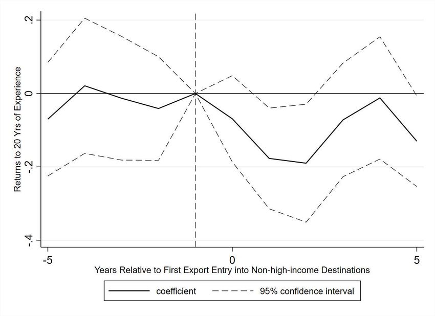
1     Introduction
It is well-known that exporters are more productive than non-exporters. This differential
is partly driven by self-selection of more capable firms into export activity (e.g., Clerides
et al. 1998). There can also be productivity improvements after exporting. For example,
Atkin et al. (2017) find that exporting improves firms’ technical efficiency in a randomized
experiment, and De Loecker (2007) shows that firms’ productivity gains may increase when
firms export to high-income countries.1 These existing studies mostly focus on firm-level
outcomes, whereas exporting may impact workers and firms jointly. It is well-documented
that workers earn higher wages at exporters than at non-exporters (Bernard and Jensen
1995). However, despite much attention to firm-level differences in lifecycle wage growth in
recent studies (Herkenhoff et al. 2018, Jarosch et al. 2018, Gregory 2019),2 little is known
about how firms’ export activity shapes workers’ lifecycle wage dynamics.
    We study empirically the relationship between a firm’s export activity and its workers’
wage profiles. We rely on Brazilian linked employer-employee data and customs records
between 1994–2010, assembling a long-run panel with detailed job information. To construct
experience-wage profiles, we measure a worker’s potential experience in the labor market as
years elapsed after schooling and then estimate how one extra year of experience within a job
(firm-worker match) affects wage growth for workers in different lifecycle stages measured
by potential experience. In principle, one more year of experience and changes in aggregate
time effects can both lead to wage changes. To resolve this well-known collinearity problem
(Deaton 1997), we apply the broadly used Heckman–Lochner–Taber (HLT) approach (e.g.,
Heckman et al. 1998, Huggett et al. 2011, Bowlus and Robinson 2012, Lagakos et al. 2018).
The centerpiece of this approach is to assume no experience returns in the end of the working
life,3 and hence old workers’ wage growth allows us to isolate time effects.
    We document three facts. First, for a person staying in a job for 20 years from the
beginning of her career, her wage growth is 85% at non-exporters and 104% at exporters,
indicating a sizeable difference of 19 percentage points in lifecycle wage growth between ex-
porters and non-exporters. Second, firm productivity proxies and firm fixed effects explain
    1
      For more evidence on the comparison of productivity levels between exporters and non-exporters, see
also Bernard and Jensen (1999), Aw et al. (2000), Van Biesebroeck (2005), Lileeva and Trefler (2010), Aw
et al. (2011), and De Loecker (2013), among others.
    2
      Herkenhoff et al. (2018) and Jarosch et al. (2018) study the effects of exposure to coworkers, and Gregory
(2019) explores the impact of firm-specific human capital accumulation.
    3
      A large number of theories of lifecycle wage growth find that there are little returns to experience in
the final working years (Rubinstein and Weiss 2006).

                                                       1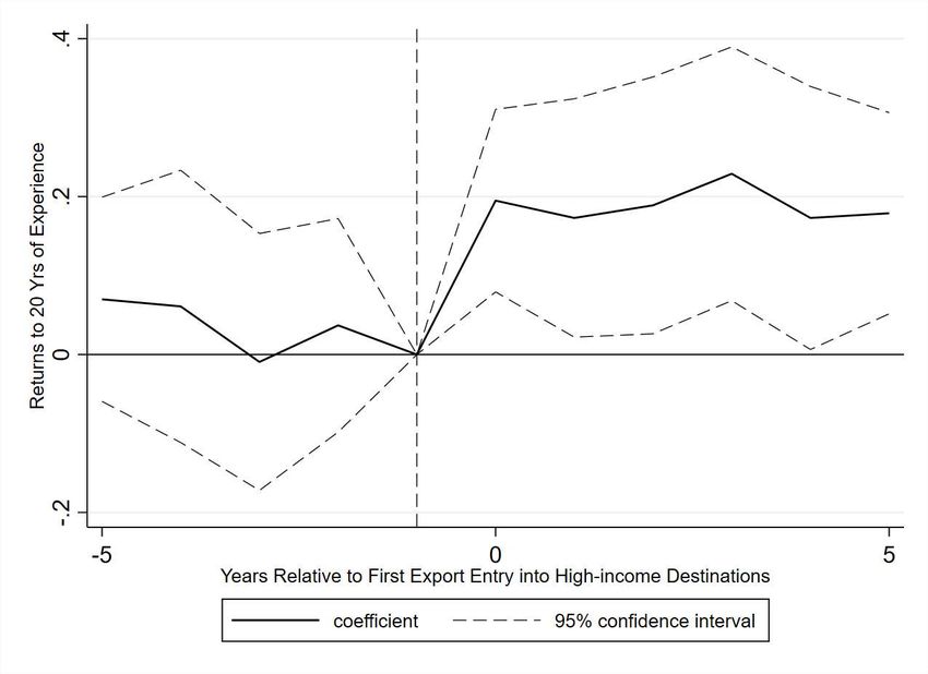
most of the differences in experience-wage profiles between exporters and non-exporters,
hinting that exporters essentially provide higher returns to experience. Third, after control-
ling for productivity proxies, labor composition, and firm fixed effects, returns to experience
are still higher when firms export to high-income destinations. We find that the increase
in returns to experience materializes immediately following firms’ entry into high-income
destinations, and this result is robust when we apply the propensity-matching approach to
lessen the endogeneity concern of export decisions.
   We show our empirical results do not rely on the HLT approach. For workers who have
been observed since a young age, instead of using age and schooling to construct potential
experience, we construct experience based on their observed employment history. Because
of possible breaks in observed employment records (due to reasons such as unemployment),
which resolve the collinearity between experience and time, we thus do not need to impose
the HLT assumption in estimation. Using this sample, we still find that previous experience
at exporters (especially those who export to high-income destinations) is more valuable than
experience at non-exporters, and that these experience effects persist after switching firms.
The estimated experience effects are of similar magnitude to our previous findings. We also
show similar results for a sample of displaced workers due to sudden closure of large firms,
as these workers’ returns to previous experience are more likely to be shaped by learning
than seniority (Jacobson et al. 1993, Dustmann and Meghir 2005).
   The impact of export activity on wage profiles can reflect human capital accumulation as
well as changes in firm-worker rent sharing, as suggested by a large literature quantitatively
studying the earnings dynamics (e.g., Bunzel et al. 1999, Rubinstein and Weiss 2006, Barlevy
2008, Yamaguchi 2010, Burdett et al. 2011, Bowlus and Liu 2013, Bagger et al. 2014, Gregory
2019). The second contribution of this paper is to develop and quantify a model with firms’
export market entry, wage renegotiations, and human capital accumulation to interpret the
data and conduct experiments.
   Our model builds on Cahuc et al. (2006), in which firms post vacancies and meet workers
by random search, and wages can be renegotiated when workers are poached by other firms.
Guided by our evidence, we embed two novel features into the model. First, we consider
that the increment in human capital per time spent increases with firm productivity and
the sales-weighted average knowledge stock in firms’ markets.4 Thus, staying in highly
productive firms (which tend to select into exporting) and being exposed to destinations
   4
    Modelling the dependence of learning returns on firm productivity is also used by Monge-Naranjo (2016)
and Engbom (2020), but they do not consider that human capital gains depend on firms’ product markets.

                                                    2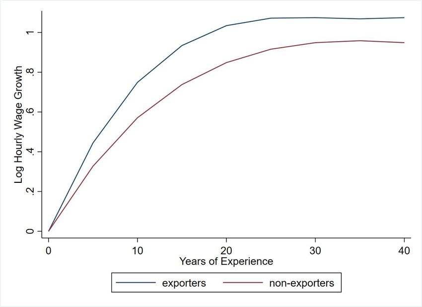
with affluent knowledge can produce faster human capital growth. Second, we consider
destinations to be heterogeneous in their levels of knowledge stock, and therefore different
combinations of destinations imply vastly different learning opportunities for workers.5
    In the model, workers’ within-job wage profiles reflect human capital growth, changes in
time allocated to human capital investment, and wage renegotiations. To understand their
relative contributions, we calibrate our model to the Brazilian manufacturing sector and
target the relevant moments to discipline the strength of wage renegotiations and human
capital investment. In the calibrated model, human capital growth can explain 70% of
the overall within-job wage profiles. However, because of diminishing returns to human
capital investment, human capital growth can only explain 40% of differences in wage profiles
between exporters and non-exporters as well as the gains in experience returns after entry
into high-income destinations. Our calibrated model is also capable to match the observed
decline in experience returns after entry into non-high-income destinations.
    We then use our calibrated model to understand the quantitative effects of trade openness.
In the first counterfactual exercise, we find that the gain in real income from autarky to
the calibrated economy is 9.50%. A large contributor is faster human capital growth with
exposure to high-income destinations—workers enjoy a 4.86% increase in average efficiency
labor due to trade openness. In the second exercise, we lower trade costs from Brazil to
specific export destinations. The gains in real income depend on destinations’ knowledge
stock and are not necessarily positive. Lowering trade costs to high-income destinations by
10% would increase Brazil’s real income by 2.70%, largely due to a 2.12% increase in workers’
average human capital. Surprisingly, lowering trade costs to non-high-income destinations
by 10% would reduce Brazil’s real income by 0.21%, mainly driven by a 0.73% decline
in workers’ average human capital. In the third exercise, we find that higher knowledge
stocks from trade partners would increase Brazil’s real income through changes in workers’
human capital. Finally, we show that assuming learning-by-doing (exogenous human capital
processes) instead of endogenous human capital investment would amplify the gains in human
capital from trade, because with no changes in time allocated to human capital accumulation,
costless human capital growth plays a larger role in explaining the wage profiles.
    This paper relates to several strands of the literature. We directly contribute to the
   5
     This setting is also in contrast with papers that incorporate trade into similar models with labor hiring
constraints (e.g., Fajgelbaum 2019, Dix-Carneiro et al. 2019), which typically model an aggregated rest of
world. Modelling multiple destinations implies a hard permutation problem for deciding the set of export
destinations from all feasible combinations, as firms’ selling decisions are interdependent across markets in
such models, and is thus computationally demanding.

                                                      3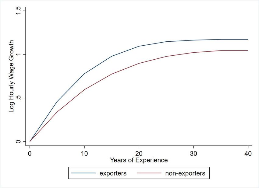
literature on learning by exporting. Recent papers show that through acquiring new knowl-
edge from exporting, firms can improve their technical efficiency (Aw et al. 2000, De Loecker
2013, Atkin et al. 2017) or understanding of export demand (Albornoz et al. 2012, Morales
et al. 2019). Few studies explore how workers may also acquire knowledge from exporting.
Exceptions are Mion and Opromolla (2014) and Muendler and Rauch (2018) who find that
employees’ previous experience at exporters is valuable for their new employers’ choices of
export markets. In contrast with these studies, we look into how export activity affects
workers’ lifecycle wage growth within the firm. Our results indicate that exporting may
enhance workers’ human capital, especially with exposure to advanced export destinations.
    We also make contact with research on lifecycle wage growth. The literature has proposed
many factors affecting lifecycle wage growth, such as job search (Bagger et al. 2014), hu-
man capital accumulation (Manuelli and Seshadri 2014), industry composition (Dix-Carneiro
2014), and match quality (Menzio et al. 2016).6 To our knowledge, our study is the first
to explore the role of a firm’s export activity in shaping its workers’ wage profiles. More-
over, much empirical work finds wage differences between exporters and non-exporters but
abstracts from experience returns (e.g., Bernard and Jensen 1995).7 We show that the ex-
porter wage premium increases with workers’ experience. Finally, recent studies highlight
the importance of lifecycle wage growth in accounting for cross-country income differences
(Islam et al. 2018, Lagakos et al. 2018). Our results imply that incentivizing exporting to
high-income may reduce the cross-country income gap.
    Our paper is also related to the literature that uses quantitative trade models with labor
market search frictions (e.g., Helpman and Itskhoki 2010, Cosar et al. 2016, Dix-Carneiro
et al. 2019, Fajgelbaum 2019). The most related paper is Fajgelbaum (2019) who also builds
on the model of labor search and wage renegotiations in Cahuc et al. (2006). Fajgelbaum
(2019) focuses on the interaction between labor market frictions and firm export decisions,
and his model abstracts from human capital and workers’ lifecycle. In contrast, our analysis
focuses on the impact of export activity on workers’ wage dynamics and thus embeds a rich
modelling of workers’ human capital accumulation and lifecycle choices.
    Finally, we connect with a large literature on international knowledge diffusion. Many
studies use macro aggregates (e.g., output, TFP, and R&D) to empirically study international
   6
      Islam et al. (2018) show how a lot of factors, such as sectors, occupations, and Internet penetration,
determine returns to experience.
    7
      The literature finds that the exporter wage premium is composed of differences in labor composition
and wage premia for workers with identical characteristics, including Schank et al. (2007), Frias et al. (2009),
and Krishna et al. (2014). These existing studies abstract from workers’ experience returns.

                                                       4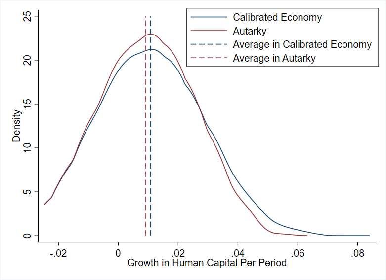
knowledge diffusion (e.g., Coe and Helpman 1995, Eaton and Kortum 1999), as reviewed by
Keller (2021), highlighting that good economic performance of outward-oriented economies
is particularly due to knowledge spillovers from foreign countries. Recent theoretical papers
also explore the relation between trade-induced knowledge diffusion and firm productivity
growth (e.g., Alvarez et al. 2013, Perla et al. 2015, Sampson 2016, Buera and Oberfield
2020).8 This literature links trade with knowledge diffusion, whereas our results highlight
that workers’ human capital accumulation may also reflect trade-induced knowledge flows.
    This paper is organized as follows. Section 2 describes our empirical findings on export
activity and experience-wage profiles, and highlights the interaction between wage profiles
and destination markets. To understand the facts and perform the quantitative analysis,
Section 3 develops a small-country model with export activity, wage renegotiations, and
human capital accumulation. Section 4 calibrates the model to match the data moments, and
Section 5 performs several counterfactual exercises to understand the role of trade openness
in affecting human capital and real income. Section 6 concludes.

2        Experience-Wage Profiles and Exporting
In this section, we document a set of stylized facts on how export activity affects experience-
wage profiles in Brazil. We show that experience-wage profiles are steeper at exporters than
non-exporters. We then show that higher experience-wage profiles at exporters reflect both
selection of more capable firms into exporting and the effects of entering more advanced
export destinations.

2.1        Data
Brazil constitutes a good case study for several reasons. First, Brazil has great data avail-
ability, as described below. Second, Brazilian exporters sell to a wide range of destinations,
allowing the exploration of how export destinations shape wage profiles. For example, in
2010, Brazil’s exports were not only directed to high-income countries (10% of total exports
to the U.S., 25% to Europe, and 4% to Japan), but also to middle- and low-income countries
(23% to Latin America, 15% to China, and 10% to Middle East and Africa). Appendix A.1
describes details of the Brazilian economy and exports during our sample period.
    We rely on the RAIS database between 1994–2010. It provides a complete depiction of
    8
        See Lind and Ramondo (2019) for a review.

                                                    5
workers employed in the Brazilian formal sector, because firms are mandated (by law) to
annually provide workers’ information to RAIS (Menezes-Filho et al. 2008).9 Each datapoint
represents a worker-firm-year observation, containing worker ID, firm ID, and workers’ in-
formation on schooling, age, hourly wage, occupation, and other demographic information.
One limitation of the data is the absence of information about the informal sector. Appendix
A.2 discusses the characteristics of the Brazilian informal sector and shows that including
informal workers in the sample may strengthen our empirical results.
We restrict our empirical analysis to manufacturing firms, which are tradable and ex-
tensively studied. In addition, we focus on full-time male workers aged between 18–65 and
employed at firms with at least 10 employees.10 If a worker has multiple records in a year,
we select the record with the highest hourly wage (Dix-Carneiro 2014). Under these restric-
tions, we obtain a sample of 72 million observations in the period 1994–2010, including 17
million unique worker IDs and 229 thousand unique firm IDs. We also provide details on
the industry and occupation classification of the database in Appendix B.
We use firm IDs to merge the RAIS data with Brazilian customs declarations for mer-
chandise exports collected at SECEX for the years 1994–2010. We define a firm as an
exporter in a given year if the firm has export transactions in that year. The SECEX data
provides which destinations and 8-digit products each firm export in each year, whereas for
1997–2000, the data also provides information on detailed export quantity and value (U.S.$).
Table 1 describes characterizations of the RAIS database, based on worker-firm-year
observations. On average, relative to non-exporters, workers at exporters are slightly older
and more educated, and earn higher hourly wages. Workers at exporters also tend to work
in cognitive occupations (professionals, technicians, and other white-collar jobs). Moreover,
exporters are much larger in terms of employment than non-exporters. These pieces of
evidence are consistent with the exporter premium typically found in the literature (e.g.,
Bernard et al. 2003, Verhoogen 2008). Finally, 49% of worker-firm-year observations are at
exporters, and thus export activity is nontrivial in our sample.
9
The ministry of labor estimates that above 90% of formally employed workers in Brazil were covered
by RAIS throughout the 1990s. The data collection is typically concluded by March following the year
of observation (Menezes-Filho et al. 2008). One benefit of this data is that the reports are substantially
accurate. This accuracy stems from the fact that workers’ public wage supplements rely on the RAIS
information, which encourages workers to check if information is reported correctly by their employers.
10
The restrictions on full-time male workers follow Lagakos et al. (2018), due to large changes in female
labor participation rates. According to the World Bank’s estimates for those aged 15+ in Brazil, female labor
force participation rate increased from 45% in 1994 to 54% in 2010, whereas male labor force participation
rate changed from 81% to 77% in the meantime. The restriction on firm size aims to avoid self-employment.
The results are quantitatively similar if we restrict the employment size to be at least 5.
6Table 1: Sample Statistics
Observations (72 million) Non-exporter Exporter
Mean S.D. Mean S.D.
workers’ characteristics:
age 31.97 9.72 32.78 9.39
schooling 8.23 3.46 9.06 3.77
log(hourly wage), Brazilian Real$ 0.67 0.77 1.20 0.96
cognitive occupations (1 if yes) 0.20 0.40 0.25 0.43
share of workers in the sample 0.51 – 0.49 –
firms’ characteristics:
log(employment) 4.51 1.56 7.05 1.71
log(exports per worker), U.S.$ – – 8.09 2.31
Note: We adjust log(hourly wage) for inflation using 1994 as the baseline year. Cognitive
occupations refer to professionals, technicians, and other white-collar workers. Firm employment
size is computed based on all workers within the firm in the raw sample (including female and
part-time workers) to reflect actual firm size. The export value data is only available in 1997–
2000, and hence log(exports per worker) is based on these four years.
In Appendix B.1, we use the raw data to present experience-wage profiles in the cross
section, showing that workers at exporters have steeper wage profiles than workers at non-
exporters.11 As there are many identification problems with this first-pass attempt, we
proceed to formally estimate experience-wage profiles.
2.2 Aggregate Experience-Wage Profiles by Export Status
Method. We consider a job as a firm-worker match and estimate experience-wage profiles
using workers’ within-job wage growth, following Bagger et al. (2014). In comparison with
using wage levels to estimate experience returns (Islam et al. 2018, Lagakos et al. 2018), this
approach takes advantage of the panel structure of our employer-employee data, controlling
for individual, firm, and match-specific fixed effects that affect wage levels and avoiding the
“incidental parameters” issue of estimating too many fixed effects (Arellano and Hahn 2007).
Another strength of focusing on within-job wage growth is that it avoids potential wage
changes related to job separations. We estimate the following regression:
X
∆ log(wit ) = φxs Ditx + (γst − γst−1 ) + ǫit , (1)
x∈X
11
We also find similar results as in the literature (Islam et al. 2018, Lagakos et al. 2018): more-educated
workers, workers in bigger firms, and workers in more sophisticated occupations have steeper wage profiles.
7where i and t represent individuals and years respectively. The subscript s is the level of
aggregation for estimating experience returns (e.g., exporters and non-exporters), which will
be specified in later implementation. ∆ log(wit ) denotes within-job wage growth, which is
log hourly wage growth from t − 1 to t for individual i within the same firm.12
As we cannot observe all workers’ full employment history, we follow Lagakos et al.
(2018) to construct a measure of potential experience in the labor market as the minimum
of age minus 18 or age minus 6 and schooling, min{age-18,age-6-schooling}. Ditx is a dummy
variable that takes the value 1 if a worker’s current potential experience is in experience
bin x ∈ X = {1–5,6–10,...}, where X is the set of 5-year experience bins. The parameter
φxs measures returns to one extra year of experience for workers in experience bin x, and
thus we allow experience returns to nonparametrically differ across stages of the lifecycle
(measured by experience bin x), because experience returns change as workers grow old.13
γst represents time effects on wage levels at time t (e.g., TFP, price levels).
Estimating equation (1) faces the well-known collinearity problem regarding experience,
individual effects, and time effects in the labor literature (Deaton 1997). This is easily seen
P
as x Ditx = 1 is perfectly correlated with the constant (γst − γst−1 ) for each aggregation
level s and time t. Intuitively, entering a new year amounts to one more year of experience
according to construction of potential experience, and wage growth over time can be induced
by experience or better aggregate economic conditions (e.g., TFP growth). To disentangle
returns to experience from aggregate trends, we adopt the HLT method used broadly in the
literature (e.g., Huggett et al. 2011, Bowlus and Robinson 2012, Lagakos et al. 2018).14 This
approach introduces a restriction on experience returns, drawing on the basic prediction of
a large number of theories of lifecycle wage growth that there are little experience returns in
the final working years, and hence workers’ wage growth in the final working years reflects
time effects.15 Implementing the HLT approach requires assumptions on two parameters: the
number of years with no experience returns, and the depreciation rate. Following Lagakos
et al. (2018), we consider 10 years at the end of the working life (31–40 years of experience)
with no experience returns and a 0% depreciation rate, and these two parameters imply the
restriction φ31−35
s + φs36−40 = 0. Appendix C.1 provides more details on the approach.
12
As the time effects γst − γst−1 depend on the aggregation level s (e.g., exporters and non-exporters),
we also require the corresponding firm status to remain constant from t − 1 to t.
13
Another common way to model experience returns is to assume a quadratic functional form (e.g.,
De La Roca and Puga 2017).
14
See Lagakos et al. (2018) for a detailed description of the method.
15
See Rubinstein and Weiss (2006) for a review of theories on lifecycle wage growth.
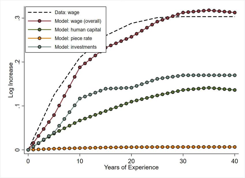
8Figure 1: Log Hourly Wage Increase by Exporters and Non-exporters
Note: This figure presents the (employment-weighted) within-industry experience-wage profiles for workers
at exporters and non-exporters, from estimating equation (1) using the Brazilian data between 1994–2010.
We assume the final 10 years with no experience returns.
Estimation Results. We apply equation (1) to estimate experience-wage profiles using
our sample. As returns to experience may differ across industries (Dix-Carneiro 2014), we
always control for industry effects when comparing wage profiles between exporters and non-
exporters.16 Figure 1 presents the estimated experience-wage profiles at exporters and non-
exporters. For a hypothetical person staying in a job for 20 years from the beginning of their
career, her wage growth is 19 percentage points higher at exporters than at non-exporters,
and the difference slightly declines to 14 percentage points after 40 years of experience.
In Appendix Figure E.1, we show that the differences in wage profiles between exporters
and non-exporters are quantitatively very similar if we assume the final 5 years with no
experience returns. An alternative value of depreciation shifts exporters’ and non-exporters’
wage profiles by the same amount and thus does not affect relative differences in wage
profiles between exporters and non-exporters. Because depreciation rates can matter for the
aggregate amount of human capital, we will calibrate and discuss the depreciation of human
capital in the quantitative analysis.
16
Specially, we estimate equation (1) separately for Brazilian workers within exporters and non-exporters,
for each 3-digit industry. We then apply identical weights (total industry-level employment) to construct
profiles for exporters and non-exporters. Consistently, we always control industry fixed effects in our firm-
level regressions below.
92.3 Firm-level Wage Profiles and Export Destinations
To understand what drives differences in experience returns between exporters and non-
exporters, we modify equation (1) to estimate firm-year-level returns to experience,
X
∆ log(wit ) = φxωt Ditx + (γωt − γωt−1 ) + ǫit , (2)
x∈X
where ω refers to a firm. The returns to experience φxωt are now firm-specific and also time-
variant to allow exploration of changes in firms’ export status, as described below. This
equation involves a large number of firm-specific parameters and usually requires grouping
firms into several groups for estimation (Bonhomme et al. 2018). To exploit the firm-level
information, instead of directly estimating equation (2), we make use of the same assumption
of the HLT method that there are no experience returns for workers in the last 10 years of
31−35 36−40
the working life, φωt + φωt = 0. Based on this assumption, the wage growth of the
last two experience bins reflects the firm-specific wage trend (γωt − γωt−1 ). Hence, we can
construct an estimate for annual returns to experience in experience bin x by
P P P
Dx ∆ log(wit ) 1 D31−35 ∆ log(wit ) D36−40 ∆ log(wit )
φ̂xωt = P it
i∈ω
x
− P it
i∈ω
31−35 + i∈ω
P it 36−40 . (3)
i∈ω Dit 2 i∈ω Dit i∈ω Dit
P x ∆ log(w )
Dit
i∈ωP it
x represents the average individual-level log wage growth between t − 1 and t,
i∈ω Dit
for workers at firm ω in both periods and in experience bin x ∈ X = {1–5,...,36–40}. By
equation (3), we control for time-varying conditions (e.g., TFP growth, demand shocks) that
alter wages for all workers within the firm. For instance, if the firm raises all workers’ wage
by the same proportion due to increased revenue after exporting, this effect will not show
up in equation (3). However, if the wage growth is relatively higher for young workers than
old workers, this relative difference will be interpreted as returns to experience.17
In Table 2, we regress firm-year-level returns to 20 years of experience on firm charac-
P
teristics. The dependent variable is 5 × x∈{1−5,...,16−20} φxω,t , measuring the hypothetical
lifecycle wage growth of a worker staying at firm ω for 20 years from the beginning of their
career, with returns to experience fixed at time t. We choose to report returns to 20 years of
experience, because many firms do not have workers in all experience bins and workers have
17
Besides estimating firm-level wage profiles, the main difference from the method in Section 2.2 is that
the previous method estimates average experience returns over time and only requires average experience
returns in the last ten years to be zero. If we also estimate time-variant experience returns φxst in Section
2.2 and restrict φ31−35
st + φ36−40
st = 0 at each time t, we can then obtain φxst similarly as in equation (3).
10Table 2: Wage Profiles and Firm Characteristics
Dep Var: Firm-year-level Returns to 20 Yrs of Experience
(1) (2) (3) (4) (5) (6)
Sample period 94–10 94–10 94–10 97–00 97–00 97–00
Exporter 0.278*** 0.018 -0.016 -0.050 -0.082 -0.050
(0.013) (0.026) (0.035) (0.073) (0.127) (0.125)
Exporter × ratio of 0.134*** 0.237**
# high-income to # total dests (0.052) (0.110)
Exporter × share of 0.180*
exports to high-income dests (0.104)
Exporter × 0.127**
log(avg GDPPC of dests) (0.062)
Exporter × -0.010 0.038 0.026 0.026
log(# total dests) (0.020) (0.053) (0.060) (0.060)
Exporter × 0.010 0.008
log(avg exports per employee) (0.030) (0.022)
Industry and Year FE Yes Yes Yes Yes Yes Yes
Firm FE No Yes Yes Yes Yes Yes
Controls No Yes Yes Yes Yes Yes
Obs 344,785 344,785 344,785 77,888 77,888 77,888
R-squared 0.007 0.318 0.318 0.488 0.488 0.488
Note: This table presents estimates from regressions of firm-year-level returns to 20 years of experience on firm character-
istics. The baseline group is non-exporters. The controls are the shares of high-school and cognitive workers in the firm’s
workforce as well as firm size. Robust standard errors are in parentheses. Significance levels: * 10%, ** 5%, *** 1%.
little returns to experience after 20 years of experience (Figure 1).
In Column (1), the independent variables are an exporter dummy (1 if a firm exports)
and a set of industry and year fixed effects. The baseline group is non-exporters. We find
that after 20 years of experience, workers’ wage increase is 27 percentage points higher at
exporters than at non-exporters, which is comparable in magnitude to the difference found
earlier (Figure 1)—19 percentage points after 20 years of experience.18
In Column (2), we control for the shares of high-school and cognitive workers in the firm’s
workforce, as labor composition can affect wage profiles (Islam et al. 2018). We further
control for firm employment size, which is associated with firm productivity (Hopenhayn
1992), and firm fixed effects, capturing time-invariant unobserved factors. Surprisingly,
18
The employment-weighted difference in returns to 20 years of experience between exporters and non-
exporters is 18 percentage points. This aligns with the result in Figure 1, which is estimated using worker-level
information and naturally puts higher weight on wage profiles at firms with larger employment size.
11after including these controls, the resulting exporters’ premium in returns to experience
declines (relative to Column (1)) and nearly vanishes. We find that only controlling for labor
composition explains 19% of the decline in the exporters’ premium, whereas only controlling
for firm employment explains 60% of the decline. These results suggest that higher returns
to experience at exporters reflect selection of better firms into exporting.
We explore the dependence of wage profiles on export destinations in Columns (3)–(6).
In Column (3), for each exporter in each year, we include the ratio of the number of high-
income destinations to the total number of export destinations. We classify countries into
high-income countries according to the World Bank classification in 2000.19 We also control
for the number of export destinations, as the scope of destinations may matter. We find that
firms that export more to high-income destinations also experience steeper wage profiles. The
coefficient suggests that other things being constant, a firm exporting solely to high-income
countries has a 13-percentage-point higher returns to 20 years of experience than an exporter
that does not sell any output to high-income countries.
In Columns (4)–(6), we exploit firm-level detailed data on export value for the 1997–2000
period. Column (4) replicates the regression of Column (3) for 1997–2000. We still find that
exporting to high-income countries increases wage profiles in 1997–2000, though the coeffi-
cients become noisier due to a smaller sample size. In Column (5), we measure an exporter’s
exposure to high-income countries by the share of exports to high-income destinations in its
total exports. We also control for export value per employee, as destination-specific effects
may originate from increased revenue due to exporting. In line with previous results, larger
shares of exports to high-income destinations significantly increase returns to experience. We
also find that controlling for export value per employee has little effects on the coefficients.
In Column (6), we measure a firm’s destination-specific exposure by using export-weighted
GDP per capita across export destinations.20 We find that exporting to destinations with
higher income significantly increases returns to experience.
In Appendix Table D.1, we replicate the results in Table 2 after controlling for duration
of workers’ previous experience at exporters and duration of the firm’s previous export par-
ticipation, as well as these durations related to high-income destinations. The coefficients of
interest barely change, suggesting that our findings are not driven by working with experi-
19
In 2000, the World Bank classifies countries into high-income countries if their GNI per capita is higher
than $9,265. To avoid that our results are affected by reshuffling of countries around the margin, we still use
our list of high-income countries in 2000 when we compute the results for other years.
20
To avoid that our results are driven by time trends of GDP per capita, we use each country’s GDP per
capita in 2000 to compute firms’ export-weighted GDP per capita across export destinations in 1997–2000.
12enced managers and coworkers (Mion and Opromolla 2014, Muendler and Rauch 2018).
In Appendix Table D.2, we divide industries into differentiated and non-differentiated
industries.21 We show that differentiated industries enjoy large and significant increases in
returns to experience due to high-income destinations, even after controlling for export value,
whereas non-differentiated industries have insignificant and small changes in returns due to
destinations. This indicates that our finding may be partly driven by workers’ human capital
accumulation, as differentiated products tend to be associated with larger scope of workers’
learning opportunities.22 Our main analysis focuses on manufacturing, whereas Brazil also
exports agricultural and mining products (see Appendix A.1). Appendix Table D.2 reports
that there are no significant experience effects of export destinations on agricultural and
mining firms, whose products tend to be more homogeneous with little scope of learning.
Before providing a quantitative analysis of possible causes of experience effects, we now
show more supportive evidence that changes in returns to experience related to high-income
destinations are caused by export activity.
2.4 Changes in Profiles around Entry to High-income Destinations
We first construct an event study to show that changes in returns to experience related to
high-income destinations materialize immediately when firms start exporting. We perform
the following regression:
=−2
τX τ =4
X X
yω,t = βτ 1{high_inc}ω,t∗ +τ + βτ 1{high_inc}ω,t∗ +τ + βpre 1{high_inc}ω,t∗ +τ
τ =−4 τ =0 τ ≤−5
X ′
+ βpost 1{high_inc}ω,t∗ +τ + Xω,t b + θω + ψj(ω,t) + δt + ǫω,t .
τ ≥5
(4)
As before, the dependent variable yω,t is firm-year-level returns to 20 years of experience. We
still control for firm fixed effects θω , industry effects ψj(ω,t) , and year effects δt . Firm-level
controls Xω,t include the shares of high-school and cognitive workers, firm size, and a dummy
variable indicating whether the firm is exporting to a non-high-income destination.
21
Using the firm-product-level export value in 1997–2000, we define a 3-digit industry to be differentiated
if its share of differentiated-product exports in total exports lies above the median across all manufacturing
industries, according to the classification of 4-digit SITC products in Rauch (1999).
22
For example, as Artopoulos et al. (2010) note in Latin America, “successfully entering markets in de-
veloped economies with differentiated products requires potential exporters to make substantial efforts to
upgrade the physical characteristics of their products and to make their marketing practices more sophisti-
cated” (p. 6).
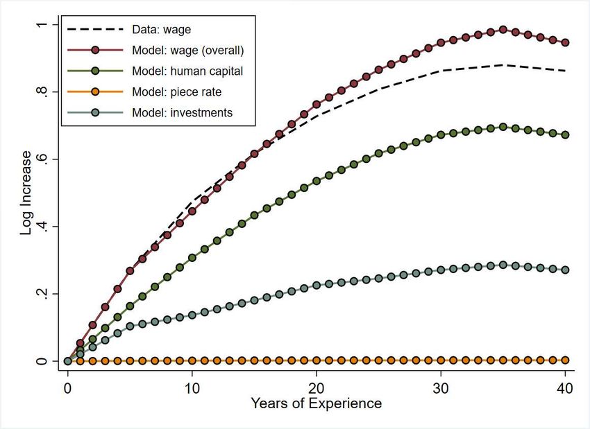
13Figure 2: Dynamics of Firms’ First Entry Into High-income Destinations
Note: The figure shows the βτ parameters from estimating equation (4). The dependent variable is firm-year-level returns to
20 years of experience. The regression controls for firm fixed effects, industry fixed effects, year fixed effects, the shares of
high-school graduates and cognitive workers in the workforce, firm size, and a dummy variable indicating whether the firm is
exporting to a non-high-income destination. To estimate the βτ parameters after entry, we require that firms remain exporting
to high-income destinations.
The βτ parameters of primary interest are coefficients on indicators for time periods
relative to the firm’s first export entry into high-income destinations at time t = t∗ (τ = 0).
We exclude an indicator for the period immediately before the firm’s export entry, and
hence the parameters represent changes in returns to experience relative to the period before
entry into high-income destinations. The coefficients are identified by firms starting as non-
exporters or exporters only to non-high-income destinations and then turning to export to
high-income destinations in our sample period. Thus, in the analysis, we focus on firms that
do not start as exporters to high-income destinations when they make first appearance in
the sample. For the βτ parameters after entry, we also require that firms remain exporting to
high-income destinations, and therefore βτ (for τ > 0) is interpreted as changes in returns to
experience for a firm that exports to high-income destinations in τ periods after first entry.
Figure 2 presents the results from estimating equation (4). After first entry into high-
income destinations, firms’ returns to experience significantly increase by 20 percentage
points, whereas experience-wage profiles do not significantly shift before firms’ export entry.
In addition, the increase in returns to experience stays roughly constant after entry, indicating
that exporting to high-income destinations is associated with persistently higher returns to
experience. Appendix Figure E.2 estimates the βτ parameters for the firm’s first export entry
14Table 3: Returns to 20 Yrs of Experience for New Exporters to High-income Destinations
Post-exporting period 0 1 2 3
(a) Outcome: returns to experience
Export entry 0.139* 0.177* 0.344*** 0.249*
(0.073) (0.095) (0.119) (0.138)
Nr treated 4,164 2,191 1,693 1,477
Nr controls 158,734 118,285 93,056 75,150
(b) Outcome: growth in returns (relative to τ = −1 period)
Export entry 0.214** 0.251* 0.065 0.383**
(0.110) (0.141) (0.187) (0.193)
Notes: The table reports the difference of returns to experience and growth in returns (relative to τ = −1 period) between
new exporters and non-exporters. The propensity score is estimated based on a Probit model, including a host of pre-
exporting (previous year) firm characteristics—returns to 20 years of experience, the shares of high-school and cognitive
workers, firm size, and export status to non-high-income destinations, as well as industry and year fixed effects. The
number of the treated and the control units on the common support decreases as there are fewer firms with future returns
to experience. Standard errors are in parentheses. Significance levels: * 10%, ** 5%, *** 1%.
into non-high-income destinations at time t = t∗ (τ = 0). We find no statistically significant
change in returns to experience after entry to non-high-income destinations.
To control for the self-selection process of exporting, we apply the propensity-score match-
ing estimator as suggested by Heckman et al. (1997) (see Appendix C.2 for details on the
approach).23 We first estimate each firm’s probability to start to export to high-income
destinations based on a Probit model. We include a host of pre-exporting (previous year)
firm characteristics, including returns to 20 years of experience, the shares of high-school
and cognitive workers, firm size, and export status to non-high-income destinations, as well
as industry and year fixed effects. The matching is based on the method of the nearest
neighbor,24 which selects a non-exporting firm which has a propensity score closest to that
of the export entrant. We find that the first moments of the covariates are not different for
the treated and the control units (balancing hypothesis, see Rosenbaum and Rubin (1984)).
Panel (a) of Table 3 reports the difference in the level of returns to experience between
new exporters and non-exporters, and Panel (b) presents the difference in growth of re-
turns (relative to τ = −1 period) between new exporters and non-exporters, which can be
interpreted as a DID estimator. These estimators are constructed in the same way as in
De Loecker (2007). We report the differences in the period of export entry (τ = 0) and
23
Previous studies have used the matching estimator to estimate the causal effects of exporting on produc-
tivity, such as Wagner (2002), Girma et al. (2003), De Loecker (2007), Konings and Vandenbussche (2008),
and Ma et al. (2014).
24
We also experiment with kernel matching or one-to-one Mahalanobis matching. We still find quantita-
tively similar results: exporting to high-income countries increases returns to experience.
15up to 3 periods after export entry for firms that remain exporting. Our results show that
exporting to high-income destinations causes an increase in returns to experience. Most of
the estimated increases in returns to 20 years of experience are significant and at around 20
percentage points, similar to our estimates in Table 2 and Figure 2.
In Appendix Table D.3, we find no significant differences in the shares of high-school and
cognitive workers between new exporters and non-exporters in the period of export entry.
This indicates that changes in labor composition may not explain increases in returns to
experience because of export entry. The subsection below explores worker-level regressions
to further confirm that our results are not driven by changes in labor composition after entry.
Appendix Table D.4 reports future effects for new exporters that stop exporting in future
periods. Increases in returns to experience become much smaller after firms stop exporting,
and the statistical significance almost vanishes. This suggests that large increases in returns
to experience are associated with continuing exporting to high-income destinations, and
there can exist some persistent effects after stopping exporting. Finally, Appendix Table
D.5 replicates Table 3 for entry to non-high-income destinations, and we find no statistically
significant changes in returns to experience after export entry.
2.5 Worker-level Results
In Appendix C.3, we construct a panel of young workers that enter RAIS under 25 years old
(arguably the beginning of the career).25 Using this restricted sample has several strengths.
First, instead of constructing potential experience based on age and schooling, we can now
construct these young people’s experience using their observed employment history in RAIS.
Second, because of possible breaks in employment history due to reasons such as unemploy-
ment (thus entering a new year does not necessarily imply one more year of experience),
their observed experience does not have the collinearity problem with year effects. Thus, we
no longer require the HLT approach in estimation.
We perform panel regression to estimate how workers’ previous work experience affects
their current wages, controlling for individual fixed effects and time effects. In comparison
with previous subsections, here we do not restrict workers’ wage growth to be within a job
in order to understand how experience affects wages after switching firms. We have three
findings. First, we find that if a new worker starts a job at exporters, she enjoys a 4.8% wage
premium relative to a job at non-exporters. If she continues to work at exporters, she enjoys
25
To extend the work history, we supplement our sample in 1994–2010 with RAIS and customs data in
1986–1993, for which we do not observe hourly wage but can construct workers’ experience.
16a 16.5% higher wage growth than working at non-exporters over 20 years of experience, in
line with the results in Section 2.2. Second, we find that the experience effects persist after
switching firms. According to the estimates, if a worker starts to work in a new firm after 20
years of experience in an exporter, she enjoys a 10.5% higher wage than previously working
at non-exporters for 20 years. Finally, we find that if a worker accumulates 20 years of
experience at exporters from the beginning of the career, working at exporters that only
export to high-income destinations would lead to a 15% higher wage growth than working
at exporters that only export to non-high-income destinations. This result is of similar
magnitude as our firm-level results in Table 2.
We further analyze a sample of displaced workers due to closure of large firms, because,
after displacement, these workers’ returns to previous experience are more likely to be shaped
by learning than seniority, following the labor literature (Jacobson et al. 1993, Dustmann
and Meghir 2005, Arellano-Bover and Saltiel 2021). We still find that previous experience
at exporters is more valuable for their post-displacement earnings than experience at non-
exporters. In particular, if a worker has accumulated 20 years of experience at exporters
before displacement, previously working at exporters that only export to high-income des-
tinations would lead to 15% higher post-displacement earnings than previously working at
exporters that only export to non-high-income destinations. This finding is of similar mag-
nitude to the results from the full sample of all young workers.
3 Model
To understand the factors behind the impact of export activity on wage profiles and its
aggregate implications, we proceed to develop and quantity a model. As suggested by our
evidence and a large literature on the earnings dynamics (e.g., Bunzel et al. 1999, Rubinstein
and Weiss 2006, Barlevy 2008, Yamaguchi 2010, Burdett et al. 2011, Bowlus and Liu 2013,
Bagger et al. 2014, Gregory 2019), we consider that wage profiles reflect human capital
accumulation as well as changes in firm-worker rent sharing.
In the model, firms meet unemployed or employed workers by random search and decide
whether to sell in foreign markets. Workers’ within-job wage grows due to endogenous
human capital accumulation and wage renegotiations. The increment in human capital per
time spent depends on the knowledge stock of destination markets, and different destinations
are heterogeneous in their knowledge stocks. We focus on a steady state in which aggregate
variables are constant. The timing of events in each period is provided in Figure 3.
17Figure 3: Timing of Events in Each Period
Firms Randomly Separate Post Vacancies Produce and Decide
from Current Workers and Hire Labor Whether to Export
Workers of Age 1 Enter Meet Firms, Accept Offers, Increase Human Capital and
and Update Wages Workers of Age T Retire
3.1 Workers, Labor Market Frictions, and Human Capital
There is a unit mass of overlapping generations of workers, with totally T cohorts. Workers
participate in the labor market from age t = 1, 2, .., T . A fraction 1/T of workers of age T
retire each period and are replaced by new entrants. Thus, the measure of workers in each
age group is 1/T . Workers have the linear utility for consumption of a nontradable final
good, and they discount the future at rate ρ. The final good is aggregated over a set of
differentiated varieties sourced from domestic or foreign origins, as we describe below.
Labor markets are subject to search frictions (Mortensen and Pissarides 1994, Pissarides
2000). At the beginning of each period, existing jobs are terminated at an exogenous rate κ.
New entrants of age 1 begin as unemployed. Unemployed and employed people then learn
of jobs randomly at rates λU and λE respectively. Let U be the total amount of unemployed
people before job search happens, and η be the search efforts of employed people relative to
unemployed people whose search efforts
are normalized
to 1. The meeting rates λU and λE
V V
are endogenously determined: λU = χ U +η(1−U )
and λE = ηλU , where U +η(1−U )
is the ratio
of the amount of all firms’ vacancies to workers’ search efforts. The function χ(·) governs
the matching process.
In each period, workers can be employed or unemployed. If employed, workers differ in
their employers and wages. As in Melitz (2003), we consider firms (employers) have different
productivity levels, drawn from a distribution Φ(z). We use productivity z to index firms.
We discuss the wage determination in Section 3.3. Workers also differ in their human capital.
New entrants of age 1 are endowed with human capital normalized to h1 = 1. Employed
workers may accumulate human capital on the job. We assume that workers’ human capital
18evolves as from age t to age t + 1:
ht+1 = (1 − δh )ht + φE (z)iαt . (5)
Here δh is the depreciation rate. The efficiency units of time spent on human capital accu-
mulation, it , are chosen to maximize the joint (firm + worker) value, as described below.
φE (z) captures the increment in human capital per unit of time spent on building skills, and
0 < α < 1 captures the degree of diminishing marginal benefits with time. Guided by our
empirical evidence, the key feature of our model is that given the same amount of time spent
on accumulating human capital, the increment in human capital is firm-specific and depends
on export destinations:
γ2
φE (z) = µz γ1 φO (z) . (6)
We model the increment as a Cobb-Douglas function of intra-firm knowledge and knowledge
outside the firm, similarly as in Monge-Naranjo (2016), with γ1 and γ2 representing the
elasticities of the increment with regard to intra-firm knowledge and knowledge outside the
firm, respectively. We use firm productivity z to proxy the stock of productive ideas within
the firm. φO (z) summarizes the set of productive ideas that are outside in firms’ markets
and available to workers in the firm. Let sn (z) be the share of sales to destination n in the
firm’s total sales, and λn denote the stock of knowledge gleaned from selling to country n.
P
Then, φO (z) = n sn (z)λn is a weighted average of destinations’ knowledge.
The intuition of this learning function is as follows. Workers can grasp knowledge from
their colleagues, through the on-site training, or by learning-by-doing, and these opportuni-
ties are more available at firms with more advanced technology (e.g., Arrow 1962, Jovanovic
and Lach 1989, Hopenhayn and Chari 1991). Directly modelling the dependence of learning
returns on firm productivity captures that better firms provide more learning, and this model
setup is also exploited in recent papers (e.g., Monge-Naranjo 2016, Engbom 2020). Learning
can also happen through interactions with the external environment. For example, firms may
adjust their product requirements for different destination markets (Verhoogen 2008, Manova
and Zhang 2012), and managers can also get new ideas by learning from the local people
they do business with or compete with (Buera and Oberfield 2020). Although the previous
literature mostly focuses on firm productivity26 and has not studied how export destinations
affect workers’ human capital accumulation, it is natural to conjecture that workers’ human
26
The idea that trade flows may affect firm productivity dates back to Grossman and Helpman (1991)
and is reviewed by Keller (2004).
19capital accumulation may also be affected by destination-specific product requirements or
personal interactions with clients. Because the share of sales to each destination in a firm’s
total sales proxies the proportion of product lines or employees devoted to that destination,
we thus weight the exposure to destinations’ technology by these sales shares.
3.2 Firm Revenues and the Trade Environment
The production side shares the central features of Melitz (2003). There is a mass M̄ of
monopolistically competitive firms with heterogeneous productivity levels z ∼ Φ(z). Without
loss of generality, we normalize M̄ = 1. Each firm produces a unique differentiated variety
using labor as the only input. Varieties are internationally traded and aggregated into a final
good in each country with a constant elasticity of substitution σ across varieties.
We consider n = 1, 2, ..., N destination markets. In particular, we index the home country
as the first market n = 1, and all other markets refer to foreign economies.27 The small-
open-economy assumption means that aggregate variables in foreign countries are invariant
to conditions at home. Because of monopolistic competition, the quantity demanded for a
variety in market n is yn = p−σ Pnσ Yn , where Pn and Yn are the aggregate price index and
quantity of the final good in market n, respectively. The price of the variety is determined
−1 1
as p = yn σ Pn Ynσ . For firms in the home country, selling to market n incurs iceberg costs τn ,
as well as fixed costs fn in terms of final goods in the home market. We assume the iceberg
and fixed costs of selling in the home market to be τ1 = 1 and f1 = 0, respectively.
For a firm with productivity z, producing one unit of good requires 1/z efficiency labor.
cv v 1+γv
To hire workers, firms need to post vacancies, and posting v vacancies costs 1+γv
units of
final goods. In the quantitative analysis, we assume γv > 0. This assumption generates the
exporter premium, because it is increasingly costly to hire new workers, and thus increased
demand due to exporting leads to larger average revenues for existing workers. Let v(z) be
the optimal amount of vacancies for firm z, as detailed below. The total number of vacancies
R Rz
is V = M̄ v(z)dΦ(z). We define F (z) = zmin v(z ′ )dΦ(z ′ )/V as the offer distribution.
We can solve the firm z’s revenue, given the total amount of efficiency labor used for
production, h(z), which is determined by the amount of vacancies and employees’ human
capital. For tractability, we assume that the firm maximizes each period’s total revenue
without consideration of the impact of export destinations on workers’ future human capital.
27
Differing from papers that model both trade and wage dynamics (e.g., Fajgelbaum 2019, Dix-Carneiro
et al. 2019), we introduce a set of foreign countries instead of one aggregated rest of world, because our
empirical analysis shows that returns to experience depend on specific export destinations.
20You can also read