Sensitivity analysis of a moored floating offshore wind turbine using a CFD based surrogate model

Sensitivity analysis of a moored
 floating offshore wind turbine
 using a CFD based surrogate
 model
 Master’s thesis in Naval Architecture and Ocean Engineering

 MIGUEL ESPINILLA
DEPARTMENT SOLADANA
 OF MECHANICS AND MARITIME SCIENCES

CHALMERS UNIVERSITY OF TECHNOLOGY
Gothenburg, Sweden 2021
www.chalmers.se

MASTER’S THESIS IN NAVAL ARCHITECTURE AND OCEAN
ENGINEERING

Sensitivity analysis of a moored floating offshore wind turbine using a CFD based
surrogate model

Miguel Espinilla Soladana

Department of Mechanics and Maritime Sciences
Division of Marine Technology
CHALMERS UNIVERSITY OF TECHNOLOGY
 Göteborg, Sweden 2021

Sensitivity analysis of a moored floating offshore wind turbine using a CFD based
surrogate model

Miguel Espinilla Soladana

© Miguel Espinilla Soladana, 2021-06-04

Master’s Thesis 2021:19
Department of Mechanics and Maritime Sciences
Division of Marine Technology
Chalmers University of Technology
SE-412 96 Göteborg
Sweden
Telephone: + 46 (0)31-772 1000

Cover:
Position of the floating platform for a 3D moored simulation at 19.33 s

Department of Mechanics and Maritime Sciences
Göteborg, Sweden 2021-06-04

Sensitivity analysis of a moored floating offshore wind turbine using a CFD based
surrogate model
Master’s thesis in Naval Architecture and Ocean Engineering
Miguel Espinilla Soladana

Department of Mechanics and Maritime Sciences
Division of Marine Technology
Chalmers University of Technology

Abstract
With increasing computational resources, the interest in high-fidelity simulations of
wave-body interaction has increased. This is the case for the CFD modelling of
Floating Offshore Wind Turbines (FOWT), as the industry moves towards
commercial farms and the need for optimization increases. Previous computational
models based on linear potential flow have shown a disagreement between the
experimental and computational motions of the moored floaters subject to wave
loading. The aim of this thesis is to help to clarify the influence of the mooring lines
in this disagreement by performing a sensitivity analysis in the mooring line stiffness.
A 1:50 scale model of a FOWT, defined by the OC5 project, is simulated using a
coupled mooring analysis using CFD. The work uses OpenFOAM for the CFD part
and Moody is used to model the mooring lines. The model is used to construct
surrogate models for the floater motions and tensions in the mooring lines using
Polynomial Chaos Expansion (PCE) in UQlab. The motions of the floater, the forces
on the mooring lines fairleads and some flow characteristics are reported. It was found
that for the wave case simulated the mooring stiffness had a negligible influence in
the periodic motions of the floater, although it could affect significantly to the mean
components of the mooring forces. The motions of the floater were found to be
underpredicted with respect to the experimental data, but in agreement with
simulations by other researchers.

Key words: FOWT, Offshore wind, CFD, OpenFOAM, Moody, UQ, gPC, mooring

Preface

In this thesis, a series of CFD simulations were made to build a surrogate model of a
floating offshore wind turbine, which was then used to perform sensitivity analysis.
The simulations were made between January and May of 2021. Chalmers Centre for
Computational Science and Engineering (C3SE) provided access to its resources to
perform the simulation in the Vera cluster. The project was carried out at the Division
of Maritime Sciences of the Department of Mechanics and Maritime Sciences.

The thesis was done under the supervision of Claes Eskilsson, Senior Researcher at
RISE, and Rickard Bensow, Full Professor at Chalmers University. This thesis would
not have been possible without the help of both of them. To their unending kindness
and understanding, as well as to the support of my family to provide this opportunity
in these trying times, I am forever grateful.

Göteborg May 2021-06-04
Miguel Espinilla Soladana

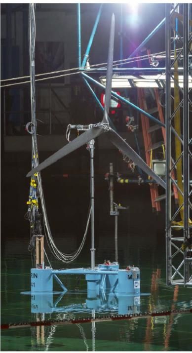
Table of contents

1 Introduction .......................................................................................................... 11
 1.1 Aim ................................................................................................................ 11
 1.2 Project Background ....................................................................................... 11
 1.3 Thesis structure ............................................................................................. 12
2 The state of the wind industry .............................................................................. 13
 2.1 Introduction to wind energy and some figures .............................................. 13
 2.2 Rationale behind using wind turbines offshore ............................................. 14
 2.2.1 Causative factors .................................................................................... 14
 2.2.2 Economical comparison ......................................................................... 16
 2.3 Foundation and mooring technologies .......................................................... 17
3 Fluid dynamics equations and discretization ....................................................... 21
 3.1 Conservation equations ................................................................................. 21
 3.2 The Navier Stokes equations ......................................................................... 22
 3.3 Turbulence modelling and boundary layers .................................................. 24
 3.4 Free surface modelling .................................................................................. 25
 3.5 Discretization process ................................................................................... 25
 3.6 SIMPLE, PISO and PIMPLE loops .............................................................. 27
4 Rigid body motion and mooring equations .......................................................... 29
 4.1 Equations for rigid body motion ................................................................... 29
 4.2 Mooring equations......................................................................................... 29
5 Uncertainty estimation method ............................................................................ 31
6 Sensitivity analysis and generalized polynomial chaos ....................................... 35
7 Methodology ........................................................................................................ 37
 7.1 Problem statement ......................................................................................... 37
 7.2 Physical properties ........................................................................................ 38
 7.3 Geometry modelling ...................................................................................... 40
 7.4 Mesh creation ................................................................................................ 43
 7.5 Case setup ...................................................................................................... 47
 7.6 Data operations .............................................................................................. 48
 7.6.1 General postprocessing .......................................................................... 48
 7.6.2 Surrogate model ..................................................................................... 48
8 Results .................................................................................................................. 50
 8.1 2D simulations............................................................................................... 50
 8.1.1 Flow field ............................................................................................... 50
 8.1.2 Model verification .................................................................................. 52

8.2 3D simulations............................................................................................... 53
 8.2.1 Flow field ............................................................................................... 53
 8.2.2 Verification ............................................................................................ 55
 8.2.3 Sensitivity analysis................................................................................. 56
 8.2.4 Motions of the floater compared to previous research ........................... 62
9 Future work .......................................................................................................... 65
10 References ............................................................................................................ 66
 Appendix A: Time until reflection calculation ........................................................ 70
 Appendix B: Boundary and initial conditions ......................................................... 72
 Appendix C: Turbulence initialization..................................................................... 73
 Appendix D: Additional mesh views ....................................................................... 74
 Appendix E: Introduction to the OpenFOAM interface .......................................... 76

Notations
Bold letters are used to denote vector fields.
Due to the variety of mathematical tools used on this project, some overlaps of
notation occur with some variables. Those variables are either used in completely
distinguishable contexts or marked with a different subscript.

Acronyms

CFD Computational fluid dynamics
FOWT Floating off-shore wind turbine
LCOE Levelized cost of energy
O&M Operations and maintenance
TLP Tension Leg Platform
OC5 Offshore Code Comparison, Collaboration, Continued, with Correlation
RAO Response Amplitude Operator
C3SE Chalmers Centre for Computational Science and Engineering
RANS Reynolds Averaged Navier Stokes
MARIN Maritime Research Institute of the Netherlands
GUM Guide to the expression of Uncertainty in Measurement
AIAA American Institute of Aeronautics and Astronautics
ASME American Society of Mechanical Engineers

UQ Uncertainty Quantification
gPC Generalized Polynomial Chaos
V&V Verification and validation

Roman lowercase letters
 Generic known vector
 Wave velocity
 Distance between floater and the far end of the simulation domain
 Internal energy
f Force, force per unit of volume, function
g Gravity acceleration
h Grid size
k Turbulent kinetic energy, index for polynomial order
 Number of grids
 Pressure, convergence order, gPC polynomial order
 Auxiliar variable for mooring equations
 Position
 Time
 Fluid velocity
 Grid weights
 Generic unknown

Roman uppercase letters
 Diagonal of M, section
 Stiffness matrix of the floater
 Damping matrix of the floater
 Young modulus
 Security factor
 Auxiliar matrix that arises during SIMPLE loop
I Turbulence intensity
L Characteristic length

 Matrix of terms arising from a discretization coefficient
 Number of faces
Q Generation per unit volume
S Surface, error function to be minimized
 Tension on the mooring line
 Uncertainty
 Volume
W Mass matrix of the floater
Z Random input for a surrogate model

Greek lowercase letters
α Volume fraction, parameter for error power expansion
γ Mass per unit length of the mooring line
ϵ Axial strain of the mooring line, discretization error
 Fluid density, probability function density
 Viscous stress tensor
μ Dynamic viscosity
λ Wavelength
σ Security factor
ν Kinematic viscosity
 Kolmogorov length scale
ω Turbulent specific dissipation rate
Greek uppercase letters
Δ Threshold parameter for error fitting to a power expansion
Γ Diffusion coefficient
Φ Generic scalar or vector field, basis function

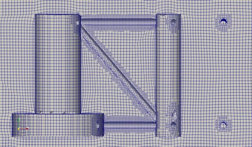
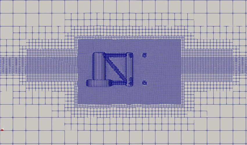
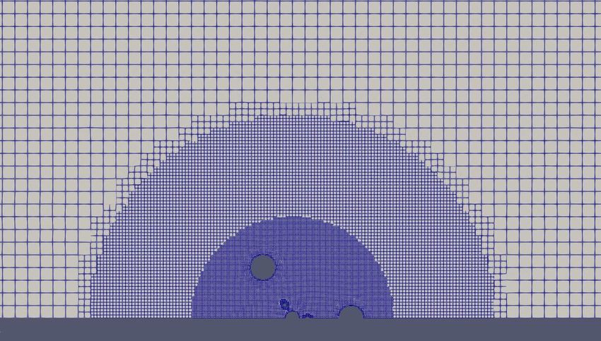
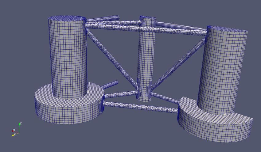
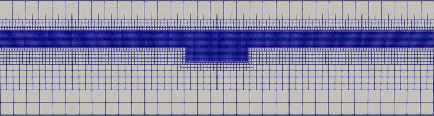
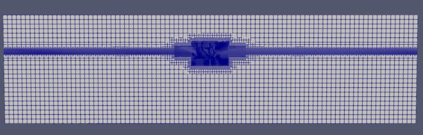
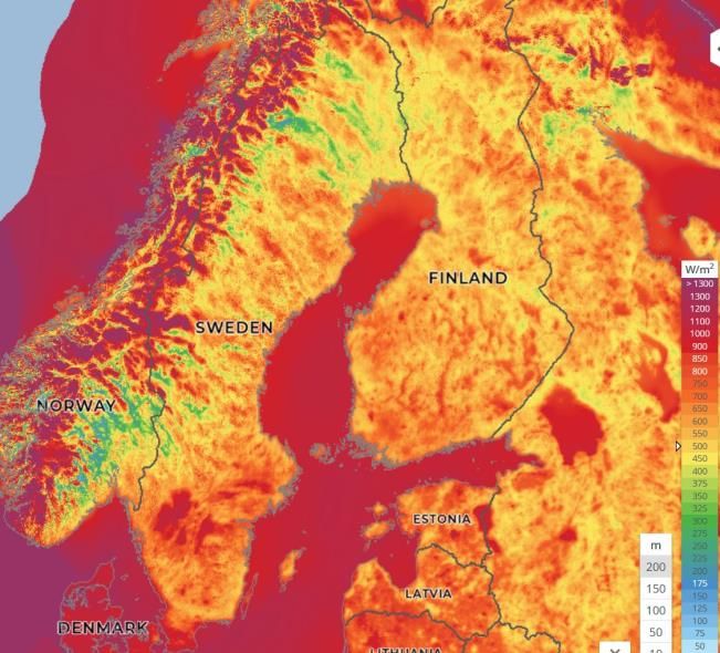
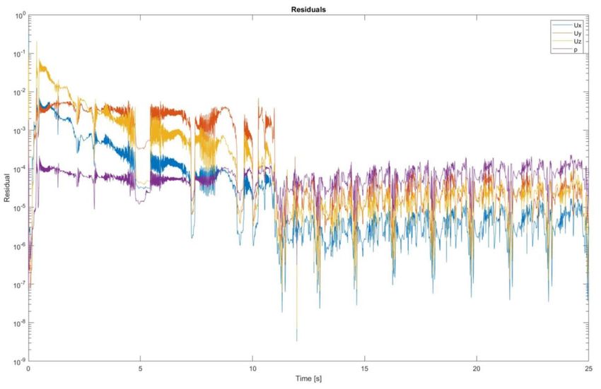
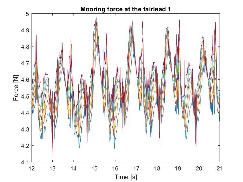
Figure index

Figure 1: Increasing share of total installed power for offshore wind [8] ................... 14
Figure 2: Mean Power Density layer of the Global Wind Atlas over the north of
Europe [12] .................................................................................................................. 15
Figure 3: Yearly average of newly installed offshore wind rated capacity [8] ............ 16
Figure 4: Total installed cost, capacity factor and LCOE for offshore (above) and
onshore (below) [9] ..................................................................................................... 16
Figure 5: Floating foundation concepts for FOWT [17] .............................................. 18
Figure 6: Number of foundations installed by type, including fixed foundations [8] . 19
Figure 7: Comparison of costs between floating and fixed offshore wind [19] .......... 19
Figure 8: Cell centred mesh (a) and node centred mesh (b) approaches [27] .............. 26
Figure 9: SIMPLE and PISO flow diagrams [30] ........................................................ 28
Figure 10: Domain of the simulation with measures and boundaries .......................... 37
Figure 11: Experimental setup at MARIN [41] ........................................................... 39
Figure 12: DeepCWind semisubmersible platform measures [41] .............................. 41
Figure 13: Mooring lines disposition [41] ................................................................... 41
Figure 14: Final CAD FOTW model ........................................................................... 42
Figure 15: SnappyHexMesh meshing process [45] ..................................................... 44
Figure 16: Domain mesh found in the literature [36] .................................................. 45
Figure 17: 2D mesh with 52.000 elements .................................................................. 45
Figure 18: Side view of the simulation domain with a mesh of 2 million cells .......... 46
Figure 19: Side view detail of the FOWT with a mesh of 2 million cells ................... 46
Figure 20: Water surface elevation at t=40.577s ......................................................... 50
Figure 21: Free surface height at the floater wave gauge for a 500.000 elements 2D
mesh ............................................................................................................................. 51
Figure 22: Computed fit (blue) vs theoretical fit (dotted line)..................................... 52
Figure 23: Flow velocity resultant in the floater region at t=19.33 s ........................... 53
Figure 24: Turbulent kinetic energy at t=19.33 s ......................................................... 54
Figure 25: Mean y+ values for a 2e6 mesh .................................................................. 54
Figure 26: Residuals for a 25 s moored simulation in a 2e6 mesh .............................. 55
Figure 27: Heave motion for the seven runs ................................................................ 56
Figure 28: Forces in the fairlead of the fairlead most exposed to the waves ............... 56
Figure 29: FFT of heave motion for the seven runs..................................................... 57
Figure 30: FFT of the mooring line 1 with a stiffness of 3.7429 kN ........................... 58
Figure 31: FFT of the mooring line 1 with a stiffness of 8.2351 kN ........................... 58
Figure 32: Example plots of surrogate models ............................................................ 59
Figure 33: Probability densitity function for the FOWT motions ............................... 60
Figure 34: Probability density function of the mooring forces .................................... 61
Figure 35: Comparison of mean motion results ........................................................... 63
Figure 36: Comparison of 1st order component motion results .................................. 63
Figure 37: Mesh detail of the FOWT surface .............................................................. 74
Figure 38: Top view of the FOWT and its surroundings ............................................. 74
Figure 39: Side view of the FOWT and its surroundings ............................................ 75
Figure 40: General file structure of and OpenFOAM case .......................................... 76
Figure 41: System folder .............................................................................................. 77

Figure 42: Code of an OpenFOAM case file ............................................................... 78

Table index

Table 1: Properties of the fluid field and the floater .................................................... 38
Table 2: Froude scaling factors .................................................................................... 39
Table 3: Scaled down mass properties of the floater ................................................... 40
Table 4: Scaled down mass properties of the mooring lines ....................................... 40
Table 5: Mooring stiffness for each simulation ........................................................... 49
Table 6: Uncertainties for each mesh........................................................................... 52
Table 7: Uncertainties of the floater motions .............................................................. 61
Table 8: Uncertainties for the mooring forces ............................................................. 62

1 Introduction
1.1 Aim
A CFD model of a moored floater has been developed in this work using the open-
source software OpenFOAM v2012 [1]. The free surface flow and the floating platform
motion have been simulated in a coupled way, using a 6 degrees of freedom model. A
non-linear dynamic mooring model has been included using the software Moody [2].
The semi-submersible floating platform has been defined using the DeepCWind
geometry, following the OC5 and subsequent OC6 project guidelines [3]. The cases
have been run in the C3SE computer cluster provided by Chalmers University of
Technology, Sweden.
The work intended to accomplish three goals:
 1. To draw conclusions out of any computational model, the convergence of the
 results should be assessed. This constituted the first objective of this work. The
 solution verification study quantified the discretization error and the associated
 uncertainty of the results, allowing to select a mesh size adequate for our
 purposes.
 2. In previous works, such as [4], an underprediction was identified between the
 motions of the floater reported in computational and in physical experiments
 with a test model. Section 1.2 expands upon this issue. The second objective of
 the project was to identify if this behaviour was still present when the mooring
 model became nonlinear.
 3. Though dynamic mooring has been routinely used in potential flow models, its
 use in conjunction with higher fidelity CFD modelling is rarer. It increases the
 complexity of the model introducing dependencies on a higher number of input
 parameters. These parameters (mooring stiffness, drag and lift coefficients of the
 mooring lines, position of the mooring fairleads, etc) are often not available with
 the desired precision due to difficulties in the measurement process, or are
 subject to significant tolerances [5]. An evaluation of the relative importance of
 said parameters in the behaviour of the mooring model was deemed interesting
 both as a way of potentially explaining the discrepancies between physical and
 computational models and to gain insight into the design drivers of these
 structures. Therefore, the second goal was to perform a sensitivity analysis on
 these parameters. Due to time constraints, only one parameter (mooring
 stiffness) could be evaluated.

1.2 Project Background
The design tools used to simulate floating offshore wind turbines are constantly being
improved. There is a great variety of methods that can be used to simulate the
hydrodynamics of the floater, as well as the aerodynamics of the tower and blades. To
compare between the options available, the International Energy Agency Technology
Collaboration Program created the Offshore Code Comparison, Collaboration,
Continued, with Correlation (OC5) project. Most of the methods were based in linear

potential flow for hydrodynamics, lumped mass for the motions of the tower and blade
element theory for aerodynamics. It was concluded that such methods introduced
simplifications to avoid paying too great of a computational price. In this way they
lacked sufficient accuracy to model the floater motions in some design cases [4].
In contrast, full CFD RANS models take into account all nonlinearities in the equations,
offering additional accuracy but increasing a great deal the computational effort.
Previously, it would have been unthinkable to use such models as an engineering tool.
However, the advances in computational capacity have made such simulations possible.
CFD RANS codes require extensive verification and validation (V&V) to become a
useful design tool. A non-exhaustive list include lift and drag on the wind turbine
blades, deformation of and loads on the structure, motions of the floater, wave
propagation, mooring line forces, sensitivity to different numerical schemes, turbulence
models, and the coupling with different tools, such as mooring models, or structural
deformation and rigid body motion solvers [6].

The Maritime Research Institute of the Netherlands (MARIN) tested a model FOWT at
1:50 scale in 2011 and 2013, and the results are still being used by many researchers for
validation. In successive investigations it was concluded that one of the main causes of
the discrepancies between the experimental results and the CFD ones could be the
mooring model. To correct this, the use of a non-linear mooring model was suggested
[4]. The program Moody, based in the discontinuous Galerkin formulation of the finite
element method, have been applied successfully as a nonlinear mooring model for
marine applications. The final objective tackled was to perform a sensitivity analysis
using a generalized Polynomial Chaos (gPC) surrogate model in order to quantify the
impact of deviations and tolerances from the nominal mooring stiffness in that model
when applied to the FOWT problem.

1.3 Thesis structure
To achieve the goals of this project the work is structured as follows. It first starts
introducing some generalities about the offshore wind field and describing the current
efforts for developing reliable floating offshore wind platforms providing examples of
some of the topologies that have been recently considered and its associated challenges.
After that, the theoretical basis is laid out, explaining the models developed for fluid,
motion and mooring simulations and the mathematical methods used to quantify
uncertainty and perform sensitivity analysis. Following this, the methodology used to
build the model, from the geometry modelling to the design considerations of the CFD
simulation are described. The postprocessing steps are commented briefly. Lastly, the
results are offered and reviewed. As an afterword, some possible future improvements
are discussed.

2 The state of the wind industry
2.1 Introduction to wind energy and some figures

Wind energy turbines use the kinetic energy available by the movement of the wind to
make a turbine spin. This rotational energy is transmitted through a shaft to an electrical
generator or any other device that can make use of it. Wind turbines face different
challenges depending on where they are placed and because of this they are classified
in:
 • Onshore wind, for turbines that are placed on land.

 • Offshore wind, for turbines that are placed on a body of water, thus requiring
 special supports. If instead of using fixed foundations floating ones are to be
 used, the resulting turbine may be called a floating offshore wind turbine
 (FOWT).
Modern use of wind energy to produce electricity started shortly after the invention of
the electric generator (1830). Electricity production started in the United Kingdom
(1887) and the US (1888), but it was in Denmark where the first modern horizontal axis
turbines were developed (1891). More than a century after that, the technology has
developed in an exponential fashion. In the last 20 years, the worldwide installed
capacity multiplied itself by 75 to reach 564 GW in 2018 [7]. A sustained reduction of
costs due to technology improvements and economies of scale as well as the recent
irruption of offshore wind ensures the continuity of the present relevance of wind
energy.
In 2020 in Europe the total installed wind power reached 220 GW and the wind farms
covered 16% of the demand of electricity. New generators accounting for 14.7 GW of
power were installed. The COVID crisis reduced the amount of new power installed,
but not by much (6% with respect of the previous year). Of the new installed generation,
only 20% was planned to be produced by offshore installations. However, this
proportion is greater than the current share for offshore of 11.4%. In the next 5 years, a
slight increase in the market share of offshore is predicted by WindEurope [8], with
24% of the new installations being offshore. Offshore is gaining traction due to a greater
resource availability and a cost reduction that is driving forward the whole wind
industry [9]. This current trend is exemplified as seen in Figure 1.

Figure 1: Increasing share of total installed power for offshore wind [8]

2.2 Rationale behind using wind turbines offshore
2.2.1 Causative factors

Offshore wind produced 3% of Europe’s electricity demand in 2020. Onshore produced
13%. Wind turbines were initially deployed on land because lower costs could be
achieved. Offshore incurs in higher cost as installation, operation and maintenance need
to be done at the sea, where the labour cost is very expensive.
There are however several advantages of going offshore [10]:

 • Increased wind resource: Figure 2 shows the mean power density (W/m^2)
 available at onshore and offshore locations in Sweden, Norway and Finland.
 Very few onshore locations can compare with the amount of power that is
 available at the sea. This is applicable to most land areas in the world. The wind
 speeds available near the surface are greatly affected by the surface roughness of
 the terrain. Water provides a comparatively smooth surface and the winds
 become stronger closer to the surface [11].

Figure 2: Mean Power Density layer of the Global Wind Atlas over the north of Europe [12]

 • More consistent wind speeds: wind tends to blow more reliably at the design
 speeds. This translates into an increment of the capacity factor.

 • Wind production is closer to consumption centres: Population centres tend to
 be in coastal areas in most countries with access to the sea. The ability to
 produce near those population centres means the energy does not need to be
 transported far away. This could alleviate the grid congestion, lower energy
 losses, and prevent potential grid overloads and blackouts.

 • Possibility of larger sized projects: as the potential sites are not restricted to a
 single location but to a large sea area. This is beneficial because it enables
 economies of scale.

 • Makes available bigger turbines: which in turn improve the total O&M cost by
 reducing the number of turbines needed to archive the same power. Figure 3
 shows this. Turbine size is difficult to scale up for onshore. In addition to the
 structural problems that arise, the size of the blades (even more than 100m),
 which are normally produced in one piece, is getting so big that it is increasingly
 difficult to transport them [13]. The possibility of water transport eliminates that
 disadvantage as the turbine blades can be manufactured along the coast and
 transported by boat to the assembly site.

Figure 3: Yearly average of newly installed offshore wind rated capacity [8]

 • Relaxes some design constrains on the turbine: turbines can rotate faster, have
 two blades or adopt a downwind configuration [11]. This is in part possible
 because, in contrast with the platforms used by the oil and gas sector, some
 safety standards can be relaxed as there is no permanent human presence nearby
 and operation and maintenance can be performed with calm seas. The noise
 intensity, a design factor with potentially harmful effects in health [14], can also
 be increased because of the same reason.

2.2.2 Economical comparison

 Figure 4: Total installed cost, capacity factor and LCOE for offshore (above) and onshore
 (below) [9]

Figure 4 offers a comparation between three important metrics to evaluate the cost
performance of offshore and onshore energy. The levelized cost of energy (LCOE) is
loosely defined as the total amount of money invested during the life cycle of a given
project (including initial investment, installation, O&M, decommission, etc) divided by
the energy produced during said product life. This metric provides a way of comparing
power plants with vastly different cost structures. By inspection, one can see that the
LCOE of offshore projects is more than double that of onshore ones.
However, the LCOE is not the only metric widely used to measure technology
performance within the electrical market. The electrical grids sustain a very delicate
balance of production and consumption which needs to be sustained day and night. The
grid operators desire (and pay for) the predictability of the power sources. The capacity
factor is defined for a given period as the amount of energy produced divided by the
amount of energy that would have been ideally produced if the generator had been
operating at rated power [15]. The high capacity factor of fossil fuels is one of the
biggest problems that are to be solved to achieve a sustainable grid, and therefore the
industry is making efforts for improving the capacity factor of the available
technologies and finding new technologies with better capacity factors.
The existence of days without wind diminishes the capacity factor of wind energy.
However, there is a great difference between offshore and onshore. For offshore energy
the capacity factor is increased, due to more reliable and constant winds on the sea. For
2019, for offshore energy the capacity was of 43.5%, whereas the onshore one was of
35.6%. However, it could be even higher. The Hywind Scotland project [16], the world
first floating wind farm, reports a capacity factor of 54%.

2.3 Foundation and mooring technologies

There are three main topologies that can be used for support structures of FOWT. They
are spar, tensioned legs platforms (TLP) and semi-submergible concepts. The current
projects deployed or in development use either one of these or a mix of several. This
section intends to briefly describe these topologies and their associated engineering
challenges. An illustration of these concepts can be found in Figure 5.

Figure 5: Floating foundation concepts for FOWT [17]

A spar foundation is stabilized by lowering the center of mass of the structure using
ballast. It offers small waterplane areas, reducing the forces it experiences. It is efficient
in harsh seas and deep waters, where the installation process is easier [18]. Some design
challenges are to balance the size of the spar buoy to match the dynamic and static
loading limits, to strengthen the turbine to withstand the heel movement produced
during operation, and the assembly of the turbine on-site. This last step involves the
complex process of raising the tower from the horizontal position in the sea [11]. The
spar concept is the one that have been used most in already installed projects, such as
the biggest current FOWT farm, Hywind Scotland.
The Tension Leg Platform (TLP) technology relies on the moorings to keep the buoyant
structure fixed to the ground. The mooring lines are inextensible, which offers a great
amount of stability, but may create problems in high or low tides, or facing extreme
waves. A loss of the mooring lines may cause the full collapse of the structure, as TLP
is not inherently stable unlike other concepts [11]. There are also installation challenges.
The hulls can experience instability when submerged before the attachment of the
mooring lines. To solve this, buoyancy aids can be added at a significant cost. New
methods are being researched to solve this [18].
The semi-submergible type of foundation consist of a floating jacket which can be made
from steel or concrete. It is moored to the floor to prevent excessive drifting. This kind
of foundation is subject to higher motions and loads, as most of the structure is on the
water surface where waves have a greater effect. Therefore the topology is designed to
allow dampening of the structure motions. The heave plates that are installed below the
floater in some topologies -including the OC5 floater- are a way of archieving that

damping. Although the fabrication process is complex and expensive, a key advantage
comes from this process: the possibility to tow the assembly. For some designs, most of
the structural components can be mounted in a dry dock in shallow waters, allowing for
a simpler installation afterwards and reducing expensive labour at the sea. This also
applies to repairs and O&M, which could be performed close to land.
As can be seen in Figure 6 spar designs are the most installed floating solutions, though
semi-submergible foundations follow closely and both are still much less common than
fixed foundations.

 Figure 6: Number of foundations installed by type, including fixed foundations [8]

Mooring is a big part of an efficient design for a FOWT. Figure 7 provides a cost
breakdown by components and processes. Although the cost of the mooring lines can
account to only 5% of the total cost of the project, including the installation, it has a
huge impact in the design of the foundations, which constitute up to 69% of the cost.

 Figure 7: Comparison of costs between floating and fixed offshore wind [19]

Mooring lines affect to the dynamic response of the FOTW. This could be a cause of
problems if the natural loading frequencies intersect the natural frequencies of the
moored floater [20]. Previous research has identified discrepancies between the
experimental movements of the FOWT and the computational experiments attributed to
a simplified mooring system. Furthermore, failure rates of mooring lines are
surprisingly high. While the industry targets useful lives of 104 to 105 years, the
observed rate of failure of single lines was of only a few dozen years. 60% of the
failures were attributed to a deficient design [5]. Further research needs to be done to
achieve confidence in the design of mooring systems for FOWT.
The material used for the mooring lines has traditionally been steel wire. The chains of
steel have the advantage of an excellent resistance to abrasion with the sea floor. Wire
rope has also been used because of its shock absorption resistance. In offshore oil and
gas platforms, some polymers have been used at very deep waters, where the weight of
steel became too expensive [11]. Some research is being done to investigate the effect
of polymers with a smaller Young modulus for shallow water applications, where steel
could prove to be too stiff. Such a variety of materials means important fluctuations in
the Young modulus for design purposes are to be expected. Even when the material of
the mooring lines is known well, differences in manufacturing can contribute to a
different stiffness values. In the model experiment of the OC5 floater [21], the
uncertainty level of the mooring stiffness reaches about 10% of its nominal value. This
same article claims that the mooring stiffness uncertainty is the single most influential
parameter in the surge response of the floater. The mooring stiffness is therefore
deemed a relevant parameter to perform a gPC sensitivity analysis with a CFD model.

3 Fluid dynamics equations and discretization
3.1 Conservation equations

Within the CFD field, there are many models that could potentially benefit from a
certain discretization or solving technique. Many conservation equations from different
fields describe the same phenomena differing only on the nomenclature. For example,
the equations for the spread of heat in a solid and the change of concentration of a
chemical species may be identical from a mathematical perspective. Therefore, it seems
like a sensible idea to refer the mathematical derivations to a general equation and then
substitute for particular variables later, instead of doing the work for each individual
equation.
This general conservation equation represents the balance between four phenomena, and
can be written as:
 ∂
 (ρΦ) + ∇ ∙ (ρ Φ) = ∇ ∙ (Γ Φ ∇Φ) + Φ (1)
 ∂ 

Where:
 1. ρ is density
 2. Φ is the scalar or vector field that is conserved
 3. is velocity
 4. Γ Φ is a dissipation rate
 5. Φ is generation of destruction of Φ
The first term in the equation is the unsteady or transient term. It allows to describe the
change of the solution with time. The second term is the convection term. It is
associated with coherent, directional movement. The third term is called the diffusion
term. It is associated with smoothing movement without a preferent direction. The
fourth one is the source term. Is associated with creation or destruction (sources and
sinks) of the quantity in the equation.
The integral form of this equation applied to a single cell, using the divergence theorem
is:
 
 ∂ (2)
 ∫(ρΦ)dV + ∑ ∫(ρ Φ) = ∑ ∫(Γ Φ ∇Φ) + ∫ Φ dV
 ∂t
 1 1

Where N is the number of surfaces of that cell. This equation still does not include any
assumption, so the solution field should be exact. To obtain an algebraic system of
equations from this conservation equation, however, assumptions need to be made. For
the FVM (Finite Volume Method) a key consideration is that the information stored in
the cell centroids must be interpolated to the surfaces to be able to evaluate the integrals.
The numerical evaluation of said integrals also create discretization error. Each term

should be discretized to reach a desired order of accuracy and some terms require
special treatment to ensure numerical stability and physical results. For this problem the
terms were discretized up to second order.

The Navier Stokes equations, as well as other equations used to model the fluid
interface and for turbulent behaviour, can be described with this framework by choosing
adequate Φ, Γ Φ and Φ .

3.2 The Navier Stokes equations

The Navier Stokes equations are the most important equations of fluid dynamics. They
describe the pressure, velocity, and internal energy of a fluid as it develops trough a
certain spatial domain during a certain time interval. They are partial differential
equations, meaning the velocity, pressure, density, and energy rates of change depend
on time and each spatial direction, adding mathematical complexity. The convective
term in the momentum equation makes the equations nonlinear. The equations are
written very generally and compactly as:

 + ∇ ∙ ( ) = 0 (3)
 
 = −∇p + ∇ ∙ ̿ ′ + ̅ (4)
 
 = −p∇ ∙ + ̿ ′ : ∇ − ∇ ∙ + + (5)
 
Where:
 1. u is the velocity vector field
 2. p is the pressure scalar field
 3. is the density scalar field
 4. is the internal energy scalar field
 5. ̿ ′ is the viscous stress tensor
 6. ̅ are the mass forces (such as gravity) per unit of volume
 7. y are heat terms produced by radiation and chemical reaction respectively
 
 8. The operator represents the material derivative:

 Φ Φ
 = + ∙ ∇Φ
 
 9. The “:” operator is the internal tensor product
 
 10. The operator represents the material derivative:
 Φ Φ (6)
 = + ∙ ∇Φ
 
 11. The “:” operator is the internal tensor product

The first equation is the continuity equation. It is always needed, as it describes
conservation of mass, which is always fulfilled. The second equation is the conservation
of linear momentum. It is derived from Newton’s Second Law of motion. Continuity
and momentum conservation equations can describe incompressible fluid. The third
equation is an energy equation. It can be formulated in terms of temperature and can be
used to describe heat transfer problems. These equations are often completed with the
equations of state of the fluid to describe compressible flow problems, giving a
complete description of almost every fluid problem relevant for industry.
For a three-dimensional case, there are very few known analytical solutions to the
Navier Stokes equations, and almost all of them are related to a very simple domain. For
complex geometry or more involved fluid behaviour, the usage of numerical methods is
always required.
For simulations involving water, such as the model of the FOWT, the fluid can be
considered incompressible ( is constant) and developing the viscous stress tensor,
substituting the mass forces by gravity, and including the turbulent quantities k and μ 
the equations become:

 ∇∙ =0 (7)

 2 (8)
 = −∇ (p + ρk) + ∇ ∙ [(μ + μ )(∇ + ∇ )] + 
 3

Where the energy equation is dropped as we assume isothermal flow. The Finite
Volume Method does not use the equations in this form, but rather requires an integral
form. A problem that arises in the numerical treatment of these equations is the lack of
the variable p in the first equation. To circumvent this, the equations are usually solved
iteratively resulting in the SIMPLE (Semi-Implicit Method for Pressure Linked
Equations), PISO (Pressure-Implicit with Splitting of Operators) or PIMPLE (Pressure-
Implicit Method for Pressure Linked Equations) loops.

3.3 Turbulence modelling and boundary layers

Turbulence is a phenomenon that happens as the small instabilities in the flow get
amplificated by the non-linear inertial terms. This causes chaotic, three-dimensional
motion that amplifies mixing and diffusion. Turbulence is usually described as a sum of
eddies of different scales. Energy is transferred between the biggest eddies to the
smallest ones in a “cascade” process, until the eddies are so small that molecular
viscosity dissipate their energy as heat. The scale of the smallest eddies that can exist is
called the Kolmogorov scale:
 1
 ν3 4
 =( ) (9)
 g

 1
 ν 2
 = ( ) (10)
 
These scales are extremely small for most engineering applications. As the element size
has to be smaller than the Kolmogorov scale to be able to resolve the eddies, the direct
approach, called Direct Navier-Stokes (DNS) is barely used as it would result in
extremely big meshes.
Most of the turbulence models used in industry work by averaging turbulent motion.
Large Eddy Simulation (LES) only simulates the largest eddies, that carry more energy,
while the smaller ones are approximated using a sub-grid model. This modelling
strategy is quite accurate but proves to be too taxing for many applications.
The Reynolds Averaged Navier Stokes family of models are an alternative with a lower
computational cost. These methods separate the variables into a mean value and a
fluctuating component and average the equations in time. The resulting averaged
equations are very similar to the original ones except for a tensor that adds six
unknowns that shall be modelled, arising from the non-linear term.
Most models assume that the components on this tensor are a linear function of the
velocity gradients (Boussinesq approximation). In that way, the problem for
incompressible flows is often simplified to compute a turbulent viscosity, μ . This can
be done using several methods. The two equation methods are popular in engineering
modelling because they offer a trade-off between accuracy, computational cost, and
stability. The − ϵ, and − ω families of models are the most used. [22]
For our application, the model used was − ω SST. It requires to solve a conservation
equation for the turbulent specific dissipation rate, ω, and for the turbulent kinetic
energy, . It offered an advantage when modelling separated flow and adverse pressure

gradients in comparison with the baseline − ω method. The equations for the − ω
SST model can be found in [23].

3.4 Free surface modelling
There are several approaches to model multiphase flows. For continuous-continuous
phase interaction, and immiscible phases, the most used one is the Volume of Fluid
method. It is based in considering each cell of the mesh as a homogeneous mixture of
both fluids with a volume fraction α, ranging from 0 to 1. A value of 0 would mean that
the cell only contains one of the fluids, and a value of one only the other one. The
properties of the cell are linearly interpolated based in α [4]. This approach allows to
solve the conservation equations only one time for both fluids. The drawback is that an
additional conservation equation is added:

 ∂α (11)
 + ∇ ⋅ (α ) = 0
 ∂ 

The discretization of the divergence term in this equation uses special schemes to
maintain a sharp interface between the fluids. If a normal upwind scheme were to be
used, there would be diffusion of α from the interface to the rest of the fluid, which
would be unphysical. The Flux Corrected Transport (FCT) is a framework in which
some of the most used schemes work. Often, high order schemes can create unwanted
oscillations in the result. To avoid this, the FCT theory proposes to blend high and low
order schemes, extending the stability of the method at high Courant numbers [24]. In
OpenFOAM, such implementation is coded through the MULES solver. Common
schemes used in this method are vanLeer, SuperBee, HRIC and CICSAM [25].

3.5 Discretization process
The objective of a discretization process is to achieve a set of equations that can be
solved with a computer. These equations, in general, are formulated in matrix form such
as:
 = (12)

To accomplish this, there are three steps that need to be followed:

• Physical modelling: The first decision that needs to be made is what is going to
 be included in the simulation. Specifically speaking, how are the boundaries of
 the domain going to look like and what are the physical phenomena that are
 going to be represented. In this simulation, for example, we are interested in the
 wave effect on the floater. If the domain boundaries were too close, the
 reflections would mix with the incoming waves and impede the retrieval of
 clean data. In this way there is a lower bound on the size of the domain. This
 kind of decisions are often highly uncertain, and should be made in accordance
 with previous research and industry experiences.

• Domain discretization: Once the geometry of the simulation is known, the
 domain should be discretized. This is done by dividing it into small partitions
 called cells, in a process called meshing. Figure 8 illustrates how a simple 2D
 mesh looks like. In general, a cell is composed of vertex, faces and a centroid. A
 cell can have any number of faces. There are two approaches to FVM meshes:
 cell-centred and node (or vertex) centred. The most used one, and the one that
 was used used, is the cell centred approach.

 Figure 8: Cell centred mesh (a) and node centred mesh (b) approaches [27]

• Equation discretization: There are several methods to discretize the governing
 equations, which can be transformed to more convenient form. The Finite
 Difference Method substitutes the derivatives for an algebraic expression
 directly on the original equations. The Finite Element Method derives a weak or
 variational form of the equations. The Finite Volume Method works with the
 integral form of the equations, which then are applied (introducing
 approximations) to each single element. Most computer software for CFD
 analysis use the FVM method, as it inherently preserves fluxes between an
 element and its neighbours [22].

3.6 SIMPLE, PISO and PIMPLE loops

The incompressible Navier-Stokes equations are a challenge to solve numerically
because they do not include an equation for pressure. The continuity equation can be
seen more as a restriction for the momentum equation. To circumvent this problem,
some manipulation is done to achieve an equation for pressure from the continuity
equation, and then the equations are solved iteratively until a combination of pressure
and velocity fields that satisfy the equations is found. A very simplified introduction to
the process is exposed here. Starting from a semi-discretized version of the original
equations [28]:
 ∇⋅ =0 (13)

 = ∇ (14)

M is a matrix of coefficients known and constant at each time step that arise from the
discretization of the momentum equation. is the vector that contains each cell
velocity. ∇ is the gradient of the pressure of each field. A H vector is defined also as:

 = − (15)

Where A is the diagonal matrix of M, so that H is only a function of u. This
decomposition is done because A is trivial to invert, which will help in later steps. With
these variables, manipulating the momentum equation and substituting in the continuity
equation yields an equation for pressure:
 ∇ ⋅ ( −1 ∇ ) = ∇ ⋅ ( −1 ) (16)

Once the pressure is known, the velocity field can be retrieved explicitly as:

 = −1 − −1 ∇ (17)

Though some methods solve the equation for pressure and velocity simultaneously,
most solvers are iterative to reduce the computational expense. The SIMPLE loop
iterates through these four equations until convergence is reached. First the momentum
equation is implicitly solved for u. Then H is computed, and the pressure equation is
solved. The velocity field is retrieved with the last equation. This is called an outer loop.
Although the last one might not seem needed, it should be noticed that in this simplified
explanation no distinction has been made between fluxes through the cell faces and

values at the cell centroids. A more rigorous mathematical description of the process
can be found in [29]. As it solves the momentum equation at each time step, the
SIMPLE algorithm is very stable.
The PISO loop starts as the SIMPLE by solving the momentum equation, computing H
and ∇ , and solving for u. However, instead solving again the momentum equation,
several iterations of the three last equations are made (inner or corrector loops). This
reduces the computational load, but it is less stable. The PIMPLE loop, a combination
of SIMPLE and PISO, uses a mix of inner and outer loops to improve stability while
keeping computational speed. Figure 9 shows a flow diagram of the methods.
When simulating a transient problem, the transient term is dominant in the equations.
This has the effect of making the simulation very stable. Hence, a fast method like the
PISO or PIMPLE is often used. The SIMPLE loop excels at stationary cases where
stability is critical, and often underrelaxation is needed to compute the loop in a stable
way.

 Figure 9: SIMPLE and PISO flow diagrams [30]

4 Rigid body motion and mooring equations
4.1 Equations for rigid body motion
The equations of motion are formulated as [6]:

 ̈ = − − ̇ (18)

W is the mass matrix, and C and D are the stiffness and the damping matrix
respectively. For our problem this D matrix is zero, as the body is assumed to be
completely rigid. The hydrodynamic forces depend on the velocity of the floater ̇
because of the Navier Stokes equations, as:

 = ∫ ∫( + ) + 
 
 = ∫ ∫( ( + )) + 
 
Where:
 1. is the pressure
 2. is the normal vector
 3. is the mooring force
 4. is the distance from the centre of mass to the element surface
 5. is the distance from the centre of mass to the mooring attachment point
In this way the equations are non-linear, and the fluid and rigid body problem are
coupled.
OpenFOAM can solve the rigid body motion equations through several methods:
Crank-Nicholson, Newmark, symplectic integrator, or even custom made solvers. The
weak stability of the coupling can be improved via acceleration relaxation (a direct
multiplier on the acceleration) or acceleration damping (where acceleration is reduced
more the higher its value is) [31]. The movement of the floater, which is a boundary
condition of the model, implies that the adoption of a moving mesh formulation must be
implemented.

4.2 Mooring equations

For the mooring, the differential equations relate the second time derivative of the
position of the mooring , with the tension and the external forces [32]:

∂2 1 ∂ (19)
 = +
 ∂ 2 γ0 ∂ γ0

 (20)
 = 0
 1+ϵ

 ∂ (21)
 =
 ∂ 

 ϵ = | | + 1 (22)

Where ϵ is the axial strain, γ0 is the mass per unit of length and is an extra variable
introduced to reduce the system to a first order system of equations. The external forces
can be divided in 4 components [5]:
 • Added mass
 • Drag
 • Buoyancy
 • Contact force
The first two arise because of the relative velocities and accelerations between the fluid
(assumed to be quiescent) and the mooring cable and are computed using the Morrison
equations. The buoyancy force is derived straightforwardly from the Archimedes
principle. The contact force is modelled as spring-damper system in the normal
direction and a Coulomb friction model in the tangential direction.
The software used to solve the mooring model is Moody [2]. This software allowed to
solve dynamics of cables, allowing the modelling of no bending stiffness chains, like
the ones used for FOWT.. The solver implements a Discontinuous Galerkin method for
spatial discretization. A few elements of high order are used to discretize the mooring
line, taking advantage of the exponential convergence of high order methods for smooth
solutions. Discretization in time is done via a third order Runge-Kutta scheme. An
introduction to the mathematical formulation, as well as verification with several test
cases relevant for offshore applications, can be found in [32].
The coupling algorithm specifies in OpenFOAM the positions of the fairleads, which
are then passed as an input for Moody. In turn, Moody will return the mooring forces as
an output for the rigid body solver. The time step of the fluid solver is in the range of
10−3 to 10−4 , whereas Moody operates in the range of 10−5 . While the rigid body
solver is still in the previous step, there is a need for interpolation of the variables that
Moody need as an input. A lagged quadratic interpolation is used to solve this. Of
practical interest is that this algorithm damps high frequency motions and therefore
needs a low enough time step in the fluid and rigid body motion solver to properly
converge

5 Uncertainty estimation method

For each experiment that is performed, be it with a physical system or a computer
simulation, differences with respect to the real system conditions will arise. For a
physical experiment, the precision and accuracy of the measuring instruments is limited,
some variables could be uncontrolled, or some process could be not well understood or
random in some way. These factors cause uncertainty in the measure, and the measure is
not complete without the uncertainty estimation.
Providing an uncertainty estimation is useful for several tasks. It has importance in
design, estimating how useful the data is to a certain design purpose. If the uncertainty
is high, the data may only be relevant for qualitative information. Lower levels of
uncertainty mean simulations can be used to study changes in the design once there is
test data available, and a very low uncertainty is associated with a direct use of the
magnitudes simulated for. Uncertainty estimation can also be a legal requirement to
comply with a standard.
For physical experiments there are well established procedures to provide an estimation
of the uncertainty of a measure. The Guide to the Expression of Uncertainty in
Measurement (GUM), is maybe the most important of such procedures. However, no
such thing exists for numerical simulations. Several procedures have been proposed by
several authors and institutions [33] [34] [35], and some guidelines published by ASME
and AIAA [36] [37], but no consensus have been reached on how to fully account for
the uncertainty of the measure [38].
Within the CFD field, two complementary ways of addressing uncertainty can be found:
 • Verification is the process used to determine whether the programming and
 computational implementation is correct or not. Code verification is performed
 by the programmers before releasing the CFD for public use. Solution
 verification is performed by the end users, and it aims to estimate the
 error/uncertainty for a computational solution even if the exact solution is
 unknown. The approach described in this section is concerned with the solution
 verification.

 • Validation, on the other hand, assesses whether the simulation agrees with the
 performance of the real system. It addresses modelling errors. A validation
 assessment cannot be done for the CFD code itself, but rather to each specific
 kind of simulation performed with it.
It has been said that verification is about solving the equations right, whereas validation
looks into solving the right equations. There are subtypes of numerical error generally
associated with verification [6], although several classifications exist:
 • Computer round-off error: The round-off error appears because of the storage
 of the numbers used in the simulation in a fixed-point way, with a fixed decimal
 length. This error is usually very small in comparison with other sources, as
 most computations are done using double precision arithmetic.