Analysis of the surface mass balance for deglacial climate simulations
←
→
Page content transcription
If your browser does not render page correctly, please read the page content below
The Cryosphere, 15, 1131–1156, 2021
https://doi.org/10.5194/tc-15-1131-2021
© Author(s) 2021. This work is distributed under
the Creative Commons Attribution 4.0 License.

Analysis of the surface mass balance for deglacial
climate simulations
Marie-Luise Kapsch1 , Uwe Mikolajewicz1 , Florian A. Ziemen1,a , Christian B. Rodehacke2,3 , and Clemens Schannwell1
1 Max  Planck Institute for Meteorology, Bundesstraße 53, 20146 Hamburg, Germany
2 Danish  Meteorological Institute, Lyngbyvej 100, 2100 Copenhagen Ø, Denmark
3 Alfred Wegener Institute, Helmholtz Centre for Polar and Marine Research,

Am Handelshafen 12, 27570 Bremerhaven, Germany
a now at: Deutsches Klimarechenzentrum, Bundesstr. 45a, 20146 Hamburg, Germany

Correspondence: Marie-Luise Kapsch (marie.kapsch@mpimet.mpg.de)

Received: 24 June 2020 – Discussion started: 10 August 2020
Revised: 21 January 2021 – Accepted: 22 January 2021 – Published: 3 March 2021

Abstract. A realistic simulation of the surface mass bal-       Superimposed on these long-term changes are centennial-
ance (SMB) is essential for simulating past and future ice-     scale episodes of abrupt SMB and ELA decreases related to
sheet changes. As most state-of-the-art Earth system mod-       slowdowns of the Atlantic meridional overturning circulation
els (ESMs) are not capable of realistically representing pro-   (AMOC) that lead to a cooling over most of the Northern
cesses determining the SMB, most studies of the SMB are         Hemisphere.
limited to observations and regional climate models and
cover the last century and near future only. Using transient
simulations with the Max Planck Institute ESM in combina-
tion with an energy balance model (EBM), we extend previ-       1   Introduction
ous research and study changes in the SMB and equilibrium
line altitude (ELA) for the Northern Hemisphere ice sheets      Increasing contributions to sea-level rise from the Green-
throughout the last deglaciation. The EBM is used to cal-       landic and Antarctic ice sheets have led to an enhanced inter-
culate and downscale the SMB onto a higher spatial resolu-      est in processes that explain past and future ice-sheet changes
tion than the native ESM grid and allows for the resolution     (see Fyke et al., 2018, for a recent review). Ice sheet mass
of SMB variations due to topographic gradients not resolved     changes are controlled by variations in the surface mass bal-
by the ESM. An evaluation for historical climate conditions     ance (SMB) and ice discharge (van den Broeke et al., 2009;
(1980–2010) shows that derived SMBs compare well with           Khan et al., 2015). The SMB is determined by mass gain
SMBs from regional modeling. Throughout the deglaciation,       due to accumulation as a result of snow deposition and mass
changes in insolation dominate the Greenland SMB. The           loss by ablation induced by thermodynamical processes at
increase in insolation and associated warming early in the      the surface and subsequent meltwater runoff (Ettema et al.,
deglaciation result in an ELA and SMB increase. The SMB         2009). Other processes resulting in ice sheet mass changes
increase is caused by compensating effects of melt and accu-    are iceberg calving and basal melting at the ice–ocean and
mulation: the warming of the atmosphere leads to an increase    ice–bedrock interfaces.
in melt at low elevations along the ice-sheet margins, while       To model the SMB, atmospheric processes associated with
it results in an increase in accumulation at higher levels as   the energy balance at the surface, as well as snow processes,
a warmer atmosphere precipitates more. After 13 ka, the in-     such as albedo evolution or refreezing, need to be simulated
crease in melt begins to dominate, and the SMB decreases.       realistically (Vizcaíno, 2014). Therefore, most of the analy-
The decline in Northern Hemisphere summer insolation af-        ses on changes and variability in the SMB have been based
ter 9 ka leads to an increasing SMB and decreasing ELA.         on observations, statistical regression, and correction tech-
                                                                niques, as well as simulations with high-resolution regional

Published by Copernicus Publications on behalf of the European Geosciences Union.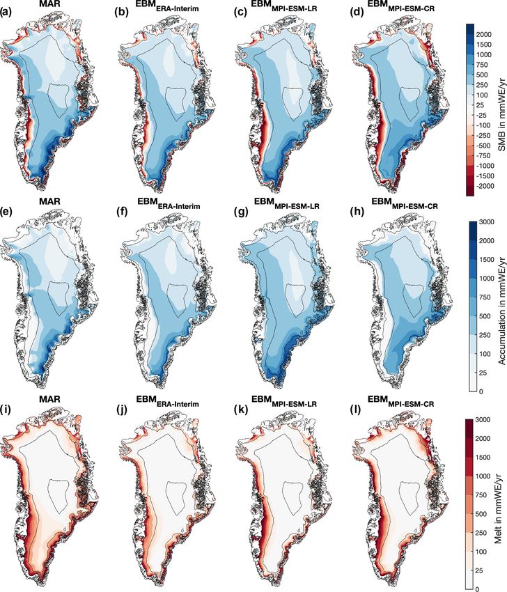
1132                                    M.-L. Kapsch et al.: Surface mass balance changes throughout the last deglaciation

climate models (RCMs) which are constrained by reanalysis           Hemisphere cooling and a significant decrease in the At-
and Earth system model (ESM) data at the lateral boundaries,        lantic meridional overturning circulation (AMOC; e.g., Keig-
and cover the last century and near future only (e.g., Fettweis     win and Lehman, 1994; Vidal et al., 1997). The significant
et al., 2008; Ettema et al., 2009; Hanna et al., 2011; Lenaerts     climate changes and the variability associated with changes
et al., 2012; Fettweis et al., 2013; Box, 2013; Fettweis et al.,    in the Northern Hemisphere ice sheets during the deglacia-
2017; Noël et al., 2018; Agosta et al., 2019; van Wessem            tion emphasize the need for a realistic representation of the
et al., 2018). However, for long-term studies of past and fu-       SMB for past and future stand-alone ice sheet and coupled
ture ice-sheet and climate changes, output from state-of-the-       climate–ice-sheet model simulations (Fyke et al., 2018).
art ESMs is used directly. It is therefore essential that ESMs         The main aim of this paper is to introduce the EBM and
are able to realistically simulate the SMB. This is specifically    apply it to long-term climate simulations. First, we introduce
challenging as ESMs exhibit biases and the horizontal resolu-       the EBM and the underlying simulations with the MPI-ESM.
tion is often not sufficient to capture small-scale climate fea-    Second, we provide a thorough evaluation of the model per-
tures, e.g., sharp topographic gradients at the ice-sheet mar-      formance for present-day climate conditions over Greenland
gins, as well as cloud, snow, and firn processes (e.g., Lenaerts    by comparing the derived SMB data set to SMBs from re-
et al., 2017; van Kampenhout et al., 2017; Fyke et al., 2018).      gional climate modeling. We then present and investigate
   In this study, SMBs are derived from transient simula-           changes and variability in the SMB and equilibrium line al-
tions of the last deglaciation with the Max Planck Institute        titude (ELA) throughout the last deglaciation and point out
for Meteorology ESM (MPI-ESM) using an energy balance               mechanisms behind the SMB and ELA changes. Here, we
model (EBM). The EBM accounts for the energy balance at             aim at exploring SMB and ELA changes under a transient
the surface, including snow processes, such as albedo evolu-        climate forcing in order to understand the mechanisms be-
tion or refreezing, and has been shown to result in a more          hind their variability at glacial timescales. As the SMB is a
realistic representation of ice volume changes than other           key parameter in controlling changes in the geometry of the
methods (e.g., positive degree day models; e.g., Tarasov and        ice sheets, this data set is available to the ice-sheet model-
Richard Peltier, 2002; Abe-Ouchi et al., 2007; Bauer and            ing community along with other forcing fields required for
Ganopolski, 2017). To thoroughly evaluate the SMBs derived          ice-sheet model simulations.
with this setup, the EBM is also applied to MPI-ESM simu-
lations of the recent historical period (1980–2010) and com-
pared to Greenland SMBs from regional modeling.                     2     Model systems and data
   This study extends the analysis of Northern Hemisphere
SMB changes to the last deglaciation (21 ka to present). The        To obtain SMB fields from long-term climate simulations,
last deglaciation was characterized by significant changes in       the MPI-ESM is used in combination with an EBM. Two
insolation and associated changes in greenhouse gas concen-         kinds of simulations were performed. First, a set of histor-
trations, ice sheets, and other amplifying feedbacks (Clark         ical simulations (1980–2010) were performed to evaluate the
et al., 2012). The large ice loss resulted in the disappear-        EBM-derived SMBs. For this, we force the EBM with output
ance of the North American and Eurasian ice sheets. In the          from historical simulations with MPI-ESM and ERA-Interim
Northern Hemisphere, only the Greenland ice sheet remains           reanalysis and compare the obtained SMBs to output from
at present. The retreat of the ice sheets during the deglacia-      the regional climate model MAR (Modèle Atmosphérique
tion resulted in about a 1 m sea-level rise per 100 years, a rate   Régional; Fettweis, 2007). Second, simulations of the last
which on average is comparable to future projections of sea-        deglaciation with prescribed ice-sheet boundary conditions
level rise (e.g., Horton et al., 2014). The collapse of the ice     were performed to investigate SMB changes under transient
sheets also resulted in significant changes in the atmospheric      climate forcing. The simulations performed for this study are
and oceanic circulation, as well as associated climate features     summarized in Table 2.
(e.g., Löfverström and Lora, 2017). Orographic changes in-
duced by the decrease in the Laurentide and Cordilleran ice         2.1    The surface energy and mass balance model
sheets led to changes in the Northern Hemisphere station-
ary wave patterns and thereby the North Atlantic jet stream,        We use the EBM to calculate and downscale the SMB from
which significantly affected the Northern Hemisphere cli-           the coarse-resolution atmospheric model grid of MPI-ESM
mate (e.g., precipitation and temperature patterns; Andres          onto high-resolution ice-sheet topographies. The main chal-
and Tarasov, 2019; Lofverstrom, 2020; Kageyama et al.,              lenge in downscaling the SMB is to realistically capture the
2020). Superimposed on these long-term changes were pe-             small-scale features of both melt and accumulation. Melt
riods of abrupt climate events. Some of the most prominent          and accumulation are highly dependent on the topographic
events are Heinrich event 1 (HE1; about 16.8 ka; e.g., Hein-        height; e.g., at a given time, low elevations might experi-
rich, 1988; McManus et al., 2004; Stanford et al., 2011)            ence melt, while higher elevations remain frozen. Projecting
and the Younger Dryas (about 13–11.5 ka; Carlson et al.,            melt and accumulation on a topography with better-resolved
2007), both of which are associated with a major Northern           vertical gradients has therefore a significant impact on the

The Cryosphere, 15, 1131–1156, 2021                                                    https://doi.org/10.5194/tc-15-1131-2021
M.-L. Kapsch et al.: Surface mass balance changes throughout the last deglaciation                                         1133

SMB. Hence, differences between the original and down-              – Near-surface air temperature and dew point are cor-
scaled SMBs are mainly a result of differences in the ele-            rected using a constant lapse rate of −4.6 K km−1 , simi-
vation rather than the horizontal grid refinement. To account         lar to the value proposed in Abe-Ouchi et al. (2007). The
for this, we employ a 3-D EBM scheme that is forced with              specific humidity, which can be used as an alternative to
high-frequency atmospheric data. The EBM scheme is an en-             the height-corrected dew-point temperature to calculate
hanced version of the energy and mass balance code that has           the latent heat flux (Bolton, 1980), is decreased with
been used to couple the ice-sheet model SICOPOLIS to a                height under the assumption that the relative humidity
previous version of MPI-ESM (Mikolajewicz et al., 2007;               stays constant throughout the atmospheric column.
Vizcaíno et al., 2008, 2010). The main improvements are
(1) an advanced broadband albedo scheme considering ag-             – The surface pressure is adjusted under the assumption
ing, snow depth dependency, and the influence of the cloud            of a typical atmospheric density and pressure profile
coverage on the thermal radiation, (2) the consideration of           p = patm0 exp(−z/Hs ), where patm0 is the pressure at
snow compaction and the vertical advection of snow and ice            the surface, z is the height, and Hs is the scale height
properties, (3) rain-induced change in the heat content of the        with a typical value of 8.4 km.
snow layers, and (4) an enhanced refreezing scheme. We fur-         – The downward longwave radiation is corrected by ap-
ther adapted the scheme by introducing elevation classes,             plying the observed constant radiation gradient of Marty
following Lipscomb et al. (2013). Calculating the SMB on              et al. (2002) and is reduced by 29 W m−2 km−1 (see also
fixed elevation levels has the advantage that the model be-           Wild et al., 1995).
comes computationally cheaper and that the obtained 3-D
fields can be interpolated onto different ice-sheet topogra-      2.1.2   Surface mass and energy balance calculation
phies (see Sect. 2.3). Note that an elevation dependence of
the SMB components is a simplified assumption and valid           Accumulation and melt determine the SMB. Accumulation
mainly for present-day Greenland. Atmospheric dynamics            is controlled by precipitation and takes place if precipitation
also significantly contribute to variations in the SMB com-       falls as snow. In the EBM, precipitation is considered as snow
ponents, specifically over present-day Antarctica. In the fol-    with a density of 300 kg m−3 when the height-corrected near-
lowing, we present the basic structure of the EBM, including      surface air temperature is lower than the freezing temperature
its improvements compared to the scheme used in Vizcaíno          of 273.15 K. Otherwise, precipitation falls as rain.
et al. (2010).                                                       The computation of melt requires a snow and/or ice model
                                                                  as the melt rate depends on the heat content of snow and the
2.1.1   Height correction                                         heat exchange between the surface snow layer and the atmo-
                                                                  sphere above, as well as the snow and/or ice layers below. To
To compute the SMB, atmospheric fields are mapped onto 24         account for this, the EBM includes a five-layer snow model
fixed elevation levels, ranging from sea level to 8000 m (we      discretized into layers of increasing thickness. The model
use irregular intervals that start with 100 m distance at the     considers only vertical exchanges because the horizontal ex-
surface and increase with height; see Table A1). To account       tent is several orders of magnitude larger than the vertical
for height differences between each of these elevation classes    extent. The snow model starts initially with a reference den-
and the surface elevation of the atmospheric model, a height      sity describing the typical exponentially increasing density
correction is applied to near-surface air temperature, humid-     with depth (Cuffey and Paterson, 2010). The top layer’s ex-
ity, dew point, precipitation, downward longwave radiation,       change with the atmosphere is computed from short- and
and near-surface density fields. The downward shortwave ra-       longwave radiation fluxes, latent and sensible heat fluxes, and
diation is kept constant as it is largely affected by atmo-       the heat release due to the immediate refreezing of rain if
spheric properties independent of elevation differences (e.g.,    the surface layer has a temperature below the freezing tem-
ozone concentration, aerosol thickness; Yang et al., 2006).       perature. Latent and sensible heat fluxes are calculated from
   The following height corrections are applied before the        the height-corrected variables using bulk aerodynamic for-
EBM calculations.                                                 mulas. The temperature of rain is assumed to be equal to
  – Total precipitation rates (liquid and solid) are corrected    the height-corrected near-surface air temperature. After up-
    in consideration of the height-desertification effect. This   dating the heat content of the surface layer, the temperature
    halves the precipitation for an orography height dif-         difference from the layer below determines the heat flux into
    ference of 1000 m above a threshold height of 2000 m          the layer below by taking density-dependent heat conductiv-
    for each grid point (Budd and Smith, 1981). Note that         ity into account (Fukusako, 1990). The heat conductivity is
    snowfall is determined from the total precipitation for       a function of density following Schwerdtfeger (1963). We
    height-corrected near-surface air temperatures below          neglect any temperature dependence of ice or snow conduc-
    0 ◦ C within the EBM.                                         tivity (Fukusako, 1990). The scheme progresses downward
                                                                  until the lowest layer is updated. The heat flux beyond the
                                                                  lowest layer is assumed to be zero, in agreement with obser-

https://doi.org/10.5194/tc-15-1131-2021                                                The Cryosphere, 15, 1131–1156, 2021
1134                                   M.-L. Kapsch et al.: Surface mass balance changes throughout the last deglaciation

vations showing that the ice or snow layer temperature below
10 m follows the long-term trend and not the seasonal cycle
(Hooke, 2005). If the ice or snow layer’s temperature exceeds      αsurface (t, dsnow ) = αsnow (t) + αbg − αsnow (t)

the melting temperature, the temperature is set to the freezing                         × exp dsnow /d̂                         (2)
point, and the related temperature excess converts the cor-
responding amount of ice or snow into liquid water. Liquid         renders this process, where αbg is the background
water penetrates into the layer below and refreezes in this        albedo, which is generally the albedo of ice, and d̂
layer as long as the layer is colder than the freezing tempera-    is 0.0024 m−1 . In the albedo parameterization, melt-
ture. Water refreezes as ice with a density of 917 kg m−3 . As     ing reduces the snow thickness, while snowfall in-
a consequence, the layer’s density grows in consideration of       creases the thickness when the precipitation rate ex-
mass conservation and eventually reaches the density of ice.       ceeds 7.23 × 10⁻¹⁰ m w.e. s−1 ≈ 2.5 cm w.e. a−1 . The maxi-
Any remaining liquid water may penetrate further downward          mum snow depth is set to 2 m w.e., which corresponds to ap-
and potentially refreezes in the layers below. Liquid water        proximately 6 m of snow. Any additional snow is still con-
that leaves the lowest layer or flows into a layer with a den-     sidered in the layer model to close the mass calculation, but
sity exceeding the pore close density of 830 kg m−3 (Pfef-         it does not impact the albedo (the snow depth is an internal
fer et al., 1991) is treated as run-off and leaves the system.     diagnostic variable).
Moreover, refreezing of meltwater heats the layer by the re-          Depending on the snow depth, melting and refreezing sur-
lease of latent heat, bringing the layer’s temperature closer to   faces have different albedo values (Table 1). If the snow
the freezing point temperature. This process eventually ter-       depth lies above or below a snow depth threshold of 0.25 cm,
minates refreezing. Rain that precipitates on the surface can      the albedos for snow and ice are used, respectively. When the
also percolate into lower layers, where it is treated as melt-     surface experiences melt, the albedo drops to the albedo of
water.                                                             snow or ice melt (αsnow-/icemelt ). When the surface refreezes,
                                                                   the albedo potentially increases (αsnowrefrz or αicerefrz ), and
2.1.3   Albedo evolution
                                                                   the aging process starts. The aging process is similar to that
The amount of incoming radiation which is available for            for snow processes as described in Eq. 1, but the albedos
heating the snow/ice layers and eventually melting is con-         for refrozen surfaces are smaller (αsnowrefrz/icerefrz ; the ref-
trolled by the surface albedo α. The albedo parametrization        erence albedo αfirn reduces to αrefrz = (2 · αsnowrfz/icerefrz +
used here differs from Vizcaíno et al. (2010). We have devel-      αsnowmelt/icemelt )/3 for refrozen snow or ice). Additionally,
oped a frequency-independent broadband albedo that com-            the process is slower (τ̂ar ). Only melted surfaces and the
bines existing parameterizations, as described in this section.    background do not experience any aging.
It represents processes neglected in conventional parameter-          Moreover, the background albedo shows a slight density
izations and covers a broader range of albedos suggested by        dependence which impacts regions of persistent high melt-
observational accounts. Note that all depths presented in the      ing and lowers the surface albedo via the background albedo.
following are water equivalent (w.e.) depths (reference den-       The background albedo is
sity of 1000 kg m−3 ).
                                                                   αbg = min (αice , q1 ρ + q2 ) ,                              (3)
   Freshly fallen snow has (in our scheme) an albedo of
0.92 (αfrsnow ; see Table 1). Snow metamorphosis processes         where q1 = −4×10⁻⁴ m3 kg−1 and q2 = 0.95, which is sim-
that change the snow’s characteristics through the growth          ilar to values published by Liston et al. (1999); see also
of larger crystals at the expense of smaller ones ultimately       Suzuki et al. (2006) for another example of this kind of pa-
transform snow into firn (Cuffey and Paterson, 2010). As a         rameterization.
result the snow albedo, αsnow (t), decreases and approaches           Furthermore, as part of our broadband albedo parame-
the albedo of firn, αfirn , which is parameterized by a time-      terization, we let varying cloud cover affect the surface
dependent exponential decay (Klok and Oerlemans, 2004;             albedo (Greuell and Konzelmann, 1994) because a higher
Oerlemans and Knap, 1998) as                                       cloud cover reflects more thermal radiation downward, which
                                                                  shifts the broadband albedo towards lower values (darker sur-
αsnow (t) = αfirn + (αfrsnow − αfirn ) exp −tsnow τ̂a ,     (1)
                                                                   face). We use the linear function of Greuell and Konzelmann
where tsnow is the time since the last snowfall and τ̂a a time     (1994) so that the maximum albedo change is 0.1 between a
constant (see Table 1). This process is here referred to as “ag-   complete overcast sky and cloud-free conditions.
ing”. Moreover, the depth of the top snow layer, dsnow (t), de-       All albedo values used in this study (e.g., for refrozen
termines how much of a potentially darker background shows         snow/ice, fresh snow, ice, firn) are tuned for a realistic rep-
through and modulates the surface albedo (Klok and Oerle-          resentation of the SMB for historical climate conditions (see
mans, 2004; Oerlemans and Knap, 1998). The equation                Sect. 3) and are listed in Table 1. The same parameters were
                                                                   applied in an EBM simulation forced with output from a
                                                                   high-resolution MPI-ESM simulation for historical climate

The Cryosphere, 15, 1131–1156, 2021                                                     https://doi.org/10.5194/tc-15-1131-2021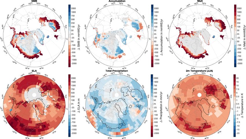
M.-L. Kapsch et al.: Surface mass balance changes throughout the last deglaciation                                                        1135

Table 1. List of constants used in the albedo scheme as part of the EBM. Please see Sect. 2.1 for further details.

      Description                                                      Symbol                 Value/comment
      Fresh fallen snow                                                αfrsnow                0.92
      Firn                                                             αfirn                  0.72
      Snow layer                                                       αsnow (t)              Between αfrsnow and αfirn ; Eq. (1)
      Ice albedo                                                       αice                   0.70
      Final albedo of snow                                             αsurface (t, dsnow )   Between αfrsnow and αice ; Eq. (2)
      Timescale of snow aging                                          τ̂a                    1/30 d−1
      Timescale for aging of refrozen snow and ice                     τ̂ar                   1/45 d−1
      Depth scale of snow layer thickness                              d̂                     0.0024 m−1 ; Eq. (2)
      Melted snow/ice                                                  αsnow-/icemelt         0.55
      Refrozen snow                                                    αsnowrefrz             0.67
      Refrozen ice                                                     αicerefrz              0.55
      Background albedo below snow layer                               αbg                    Eq. (2); defined in Eq. (3), where αbg ≤ αice
      Density dependence of background albedo parameter, factor        q1                     −4 × 10⁻⁴ m3 kg−1
      Density dependence of background albedo parameter, offset 1      q2                     0.95
      Background albedo below refrozen layer                           αbg                    αbg = αice for snow aging; Eq. (1)

conditions within the scope of SMB model inter-comparison                 eral circulation model ECHAM6.3 (Stevens et al., 2013), the
(Fettweis et al., 2020). The results showed that the derived              land surface vegetation model JSBACH3.2 (Raddatz et al.,
SMBs were very similar to observations in terms of the SMB                2007), and the primitive equation ocean model MPIOM1.6
mean climate, as well as the SMB trend (2003–2012).                       (Marsland et al., 2003). Two different resolutions are used
                                                                          for the simulations. (1) For calculating the SMB over the last
2.1.4    Vertical advection and density evolution                         deglaciation, MPI-ESM is used in its coarse-resolution (CR)
                                                                          setup, hereafter referred to as MPI-ESM-CR. In this setup,
For a non-zero SMB, the thickness of the uppermost layer                  ECHAM6.3 has a T31 horizontal resolution (approx. 3.75◦ )
of the snow model would change. To compensate for that,                   with 31 vertical hybrid σ levels which resolve the atmo-
a simple 1-D advection scheme conserving heat and mass is                 sphere up to 0.01 hPa (Stevens et al., 2013), and MPIOM1.6
applied. In the case of surface ablation, the densities and tem-          has a nominal resolution of 3◦ with two poles located over
peratures are advected upward. As the lower boundary condi-               Greenland and Antarctica (Mikolajewicz et al., 2007). The
tion, we assume an inflow of ice with a density of 917 kg m−3             selected setup is a compromise between computational fea-
and a temperature of the lowest model layer. In the case of ac-           sibility and model resolution. (2) We additionally use a simu-
cumulation, an inflow of snow with a density of 300 kg m−3                lation with the low-resolution version of MPI-ESM1.2, here-
and a temperature of the height-corrected near-surface air                after referred to as MPI-ESM-LR, in which ECHAM6.3 has
temperature is assumed as the upper boundary condition. To                a T63 spectral grid (approx. 1.88◦ ) with 47 vertical levels,
account for snow compaction, we introduce the aforemen-                   and MPIOM features a 1.5◦ nominal resolution. For model
tioned reference density profile (Cuffey and Paterson, 2010).             details, see Mauritsen et al. (2019).
If the density of the downward-advected snow into a layer is
smaller than the reference density in that layer, the density of
                                                                          2.3    Transient MPI-ESM climate simulations
the advected snow is set to the reference density, and the flow
to the layer below is reduced accordingly to conserve mass.
Once the reference density is reached in all layers, mass flows           We performed different simulations with the MPI-ESM-
out of the bottom layer and is removed from the system. As a              CR setup: (1) simulations to investigate the SMB through-
consequence of this procedure, the density in each layer lies             out the last deglaciation, starting at 26 ka until the present
always between the reference density (in the case of perma-               (here, defined as 1950), and (2) simulations to evaluate the
nent snow accumulation) and the density of pure ice (in the               SMB for historical climate conditions (see Table 2). For
case of permanent ablation).                                              the deglaciation experiment, the model was started from a
                                                                          spun-up glacial steady state and integrated from 26 ka un-
2.2     The Max Planck Institute Earth System Model                       til the year 1950 with prescribed atmospheric greenhouse
                                                                          gases (Köhler et al., 2017) and insolation (Berger and Loutre,
The simulations in this study are performed with the Max                  1991). The ice sheets and surface topographies were pre-
Planck Institute for Meteorology Earth System Model (MPI-                 scribed from the GLAC-1D (Tarasov et al., 2012; Briggs
ESM, version 1.2; see Mikolajewicz et al., 2018; Maurit-                  et al., 2014) reconstructions (Kageyama et al., 2017, see stan-
sen et al., 2019), consisting of the spectral atmosphere gen-             dardized PMIP4 experiments). We focus our analysis on the

https://doi.org/10.5194/tc-15-1131-2021                                                            The Cryosphere, 15, 1131–1156, 2021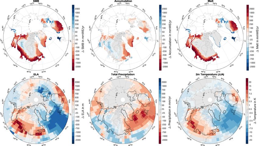
1136                                    M.-L. Kapsch et al.: Surface mass balance changes throughout the last deglaciation

last 21 kyr of the simulation. Hereafter, this simulation is re-    for their climatic impacts for present-day climate conditions.
ferred to as MPI-ESM-CR deglaciation experiment. All forc-          Specifically, we apply time-varying greenhouse gases (CO2 ,
ing fields are prescribed every 10 years and initiate changes       N2 O, CH4 ), volcanic forcing, ozone, tropospheric aerosols,
in the topography and glacier mask, as well as modifications        and land-cover changes (see Jungclaus et al., 2010; Maurit-
of river pathways, the ocean bathymetry, and the land–sea           sen et al., 2019). For the evaluation, only the years 1980–
mask (Riddick et al., 2018; Meccia and Mikolajewicz, 2018).         2010 are used, which allows for a sufficient adjustment of
Freshwater from changing ice sheets is calculated from the          the model to changes in the forcing. We hereafter refer to this
thickness changes in the ice-sheet reconstructions for each         simulation as the MPI-ESM-CR historical experiment. Note
grid point. For grid cells over land, meltwater is distributed      that changes in the topography due to ice sheets are small
through the hydrological discharge model, and over ocean it         between 950 years BP and 2010. Hence, we expect only a
is discharged into the adjacent ocean grid cells. Ocean cells       minor impact on the obtained SMBs.
that become land due to changes in the sea level are initial-          Additionally, we performed a deglacial, last millennium,
ized with the same vegetation form as the adjacent grid cells,      and historical simulation in which ice sheets and topogra-
while land cells that are deglaciated are covered with bare         phies are prescribed from ICE-6G reconstructions (Peltier
soil. After this initialization, the vegetation of the grid cells   et al., 2015), an alternative reconstruction often used as
evolves interactively with JSBACH. Anthropogenic forcing,           boundary forcing in deglacial simulations (Kageyama et al.,
such as land use, is turned off in this simulation. For calculat-   2017). Results from these simulations, hereafter referred
ing the SMB, relevant variables of the atmospheric compo-           to as MPI-ESM-CRIce6G experiments, are shown in Ap-
nent of MPI-ESM1.2 are written out hourly throughout the            pendix A1 and emphasize differences in the SMB and rel-
simulation. Using the obtained atmospheric fields within the        evant fields due to different ice-sheet boundary conditions.
EBM (see Sect. 2.1) results in 3-D SMB fields which are then        While the SMB response to the climate forcing in these sim-
interpolated onto the GLAC-1D topography and ice mask               ulations is qualitatively similar to the MPI-ESM-CR simula-
(Tarasov et al., 2012). Computing a 3-D SMB also allows             tions forced with GLAC-1D reconstructions, differences in
us to calculate the equilibrium line altitude (ELA), the ele-       the freshwater runoff between the reconstructions lead to a
vation at which the SMB equals zero. At heights above the           different climate response in the model simulations.
ELA, it is thermodynamically possible to accumulate snow               For a thorough evaluation of the EBM and in order to
throughout the year and form an ice sheet or glacier. At el-        investigate the effect of model resolution on the historical
evations below the ELA, melt dominates accumulation, and            SMB, we additionally calculate the 3-D SMB fields from a
no ice sheet can form. Here, the ELA is calculated in each          CMIP6 (Wieners et al., 2019) historical simulation with the
grid point, hence, resembling a potential ELA. It is a proxy        MPI-ESM-LR setup (see Sect. 2.2; Mauritsen et al., 2019;
for climate changes affecting the ice sheets. As the ELA es-        Wieners et al., 2019). The simulation allows us to further
timate is calculated on the native model grid, it is more con-      evaluate the EBM and to investigate differences in SMBs in
sistent with the model physics and boundary conditions used         regards to the spatial model resolution, as well as differences
in the simulations than the downscaled SMB. Hence, inte-            due to the underlying topographies. This simulation is here-
grated values of the ELA are less sensitive to changes in the       after referred to as MPI-ESM-LR historical experiment.
ice-sheet mask than those of the SMB.                                  The 3-D fields derived for all historical control simulations
   For the evaluation of the derived SMBs under histori-            are 3-dimensionally interpolated onto the ISMIP6 topogra-
cal climate conditions, we branched off a last millennium           phy and masked with the ISMIP6 ice mask (see Sect. 2.4;
simulation at 950 years BP (years before present) from the          Nowicki et al., 2016; Fettweis et al., 2020).
deglaciation experiment. Within PMIP, last millennium sim-
ulations are used to provide a seamless transition between          2.4   Evaluation data
the last deglaciation and the historical period (Jungclaus
et al., 2017). For the simulation, topography, land–sea and         To evaluate the EBM with respect to the atmospheric forc-
glacier masks, river pathways, and the ocean bathymetry are         ing data and its resolution, we additionally force the EBM
taken from the deglaciation experiment and kept constant            with ERA-Interim reanalysis data from the European Center
at 950 years BP. Other forcing fields are adopted accord-           for Medium-Range Weather Forecasts (ECMWF; Dee et al.,
ing to the PMIP3 standard protocol for the last millennium          2011). ERA-Interim was chosen as it is used as boundary
simulations (Schmidt et al., 2012) and updated every year.          forcing in the RCM simulations, which are used for a more
The forcing fields for the years 1850 to 2010 are taken from        thorough evaluation and are introduced at the end of this sec-
the CMIP6 simulations (see Mauritsen et al., 2019). For the         tion. For comparison, we interpolate the ERA-Interim de-
years beyond 2010, the forcing fields in the desired resolu-        rived 3-D SMB fields onto the ISMIP6 topography and mask
tion were not available at the time of the analysis. Overall,       it with the ISMIP6 ice mask (see Sect. 2.3). ERA-Interim is
the applied forcing allows for a more realistic treatment of at-    available as 6-hourly data at a 0.75◦ × 0.75◦ horizontal res-
mospheric processes associated with changes in, e.g., ozone,        olution. ERA-Interim assimilates a great fraction of in situ
aerosols, CO2 concentrations, and land use, and it accounts         and remote sensing observations, making it one of the best re-

The Cryosphere, 15, 1131–1156, 2021                                                    https://doi.org/10.5194/tc-15-1131-2021
M.-L. Kapsch et al.: Surface mass balance changes throughout the last deglaciation                                                                                 1137

Table 2. Simulations performed, as described in Sect. 2.3. For the deglaciation experiments, the topography and ice sheets are taken from
reconstructions and change throughout the simulation. For the historical and last millennium simulations, those fields remain constant through
time.

                     Period              Experiment name               Topography/ice-sheet mask          Spin-up
                     Deglaciation        MPI-ESM-CR                    GLAC-1D (transient)                26 ka steady state
                     (26–0 ka)           MPI-ESM-CRIce6G               ICE-6G (transient)                 26 ka steady state
                     Historical          MPI-ESM-CR                    GLAC-1D (950 years BP)             Last millennium simulation
                     (1850–2010)         MPI-ESM-CRIce6G               ICE-6G (950 years BP)              Last millennium simulation
                                         MPI-ESM-LR∗                   CMIP6                              Preindustrial steady state
                   ∗ This simulation contributed to CMIP6 (see Sect. 2.3).

analysis products available (Cox et al., 2012; Zygmuntowska                       Table 3. Average and standard deviation of the annual SMB simu-
et al., 2012). However, as reanalysis data sets are model prod-                   lated with MAR and the EBM forced with ERA-Interim and a his-
ucts, they exhibit biases specifically for variables associated                   torical MPI-ESM simulation for the years 1980–2010. The annual
with small-scale processes and areas where in situ observa-                       SMB values are interpolated onto the ISMIP6 ice-sheet topogra-
tions are sparse (e.g., precipitation, clouds; Stengel et al.,                    phy (see Sect. 2.4) except for RACMO∗ . The standard deviation
                                                                                  reflects the interannual variability. Units are in gigatonne per an-
2018). These biases are not unique to ERA-Interim but can
                                                                                  num (Gt a−1 ). Accumulation is calculated as residual of the SMB
be found in other reanalyses (Miller et al., 2018). Relevant                      and melt.
biases for this study are discussed in Sect. 3.
   Additionally, we compare the obtained SMB data sets                              Model                                       SMB         Melt      Accumulation
from the MPI-ESM historical experiments to SMBs derived
                                                                                    MAR                                  340 ± 122         −548                    888
with MAR (version 3.9.6). For a detailed description of MAR
                                                                                    RACMO∗                               367 ± 108         −540                    907
and its setup, see Fettweis et al. (2017, 2020). The MAR sim-                       EBMERAI                              344 ± 140         −288                    632
ulation used in this study was run at a 15 km horizontal reso-                      EBMMPI-ESM-LR                         351 ± 83         −311                    663
lution with ERA-Interim boundary forcing (Dee et al., 2011)                         EBMMPI-ESM-CR (Glac1D)               275 ± 107         −495                    770
and interpolated onto the ISMIP6 topography (Nowicki et al.,                        EBMMPI-ESM-CR (Ice6G)                 307 ± 71         −440                    747
2016), as described in Fettweis et al. (2020).                                    ∗ RACMO data are provided on a slightly different topography with 1 km horizontal
                                                                                  resolution (see Noël et al., 2019, for details); the impact of the underlying topography
                                                                                  on the SMB values is expected to be small.
3   Greenland surface mass balance under historical
    climate conditions

For the Greenland ice sheet, a thorough evaluation of the ac-                        The SMBs from EBMERAI , EBMMPI-ESM-LR , and
cumulation and surface energy budget that determines sur-                         EBMMPI-ESM-CR show good agreement with SMBs from
face melt is conducted under historical climate conditions                        MAR for the historical period. The largest mass loss occurs
(1980–2010). Variables derived from the EBM simulations                           along the low-elevation areas close to the coasts, with
forced with output from ERA-Interim and the historical MPI-                       maxima in the west and southwest of Greenland. The largest
ESM simulations are compared to SMBs from MAR. SMB,                               mass gain is evident in the higher-elevation areas in the
accumulation, and melt data sets are presented on the same                        west and southeast of Greenland. For all simulations, the
ISMIP6 topography (see Sect. 2.3 and 2.4). In the follow-                         mass changes over northern central Greenland are small due
ing, accumulation is defined as mass gain due to snow de-                         to low precipitation at high elevations (see Fig. 2). Also,
position and melt as mass loss due to ablation (often re-                         the gradients between areas of the most pronounced mass
ferred to as runoff). Refreezing processes are considered in                      loss and gain are qualitatively similar in all simulations.
the melt estimate (see Sect. 2.1). All variables obtained us-                     Differences in the SMB fields are largest along the coasts
ing the EBM are hereafter referred to as EBMMPI-ESM-CR ,                          in the southeast and west of the Greenland ice sheet. These
EBMMPI-ESM-LR , and EBMERAI for the EBM simulations                               differences are likely a result of the forcing data, model
forced with the historical simulations of both MPI-ESM in                         resolution (about 3.75◦ , approx. 250 km over Greenland for
coarse (CR) and low (LR) resolution and ERA-Interim re-                           MPI-ESM-CR; 1.88◦ , approx. 120 km for MPI-ESM-LR;
analysis. The annual mean SMB averaged over 1980–2010                             0.75◦ , approx. 50 km for ERA-Interim; and 15 km for MAR),
and the Greenland integrated value are shown in Fig. 1 and                        and underlying topographies (Fig. 2). Differences between
Table 3 for each of the simulations. The corresponding plots                      MAR and EBMERAI are generally smaller than differences
for the MPI-ESM-CRIce6G simulation are shown in Fig. A1.                          between MAR and EBMMPI-ESM-CR or EBMMPI-ESM-LR
                                                                                  because ERA-Interim data were used as boundary forcing

https://doi.org/10.5194/tc-15-1131-2021                                                                         The Cryosphere, 15, 1131–1156, 2021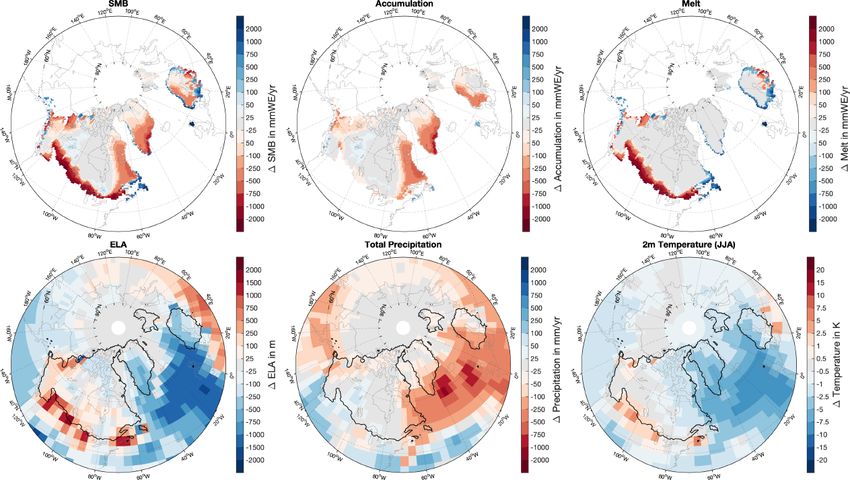
1138                                    M.-L. Kapsch et al.: Surface mass balance changes throughout the last deglaciation

Figure 1. (a–d) SMB, (e–h) accumulation, and (i–l) melt from (a, e, i) MAR and EBM simulations forced with (b, f, j) ERA-Interim,
(c, g, k) MPI-ESM-LR, and (d, h, l) MPI-ESM-CR for historical climate conditions. The values are averaged over 1980–2010. All variables
are interpolated on the ISMIP6 topography and shown only for glaciated points. Note that accumulation is obtained as the residual of SMB
minus melt as MAR does not provide accumulation as a direct output variable. Black contours mark surface elevations of 0, 1000, 2000, and
3000 m.

for the MAR simulation. Comparing SMBs derived from                    individually to better understand the mentioned differences
EBMMPI-ESM-CR and EBMMPI-ESM-LR shows that specif-                     between the simulations.
ically the SMB differences in the north of the Greenland
ice sheet, associated with more melt in EBMMPI-ESM-CR                  3.1   Accumulation
along the coasts and enhanced accumulation in the center
of the ice sheet compared to EBMMPI-ESM-LR , are partly                Accumulation patterns in MAR and the three EBM simula-
a consequence of the model resolution. In the following,               tions are similar. However, they show some differences in
we investigate the components that determine the SMB                   the low-elevation areas in the southeast of the ice sheet and
                                                                       the northern plateau (Fig. 1). Integrated over the ice sheet,

The Cryosphere, 15, 1131–1156, 2021                                                        https://doi.org/10.5194/tc-15-1131-2021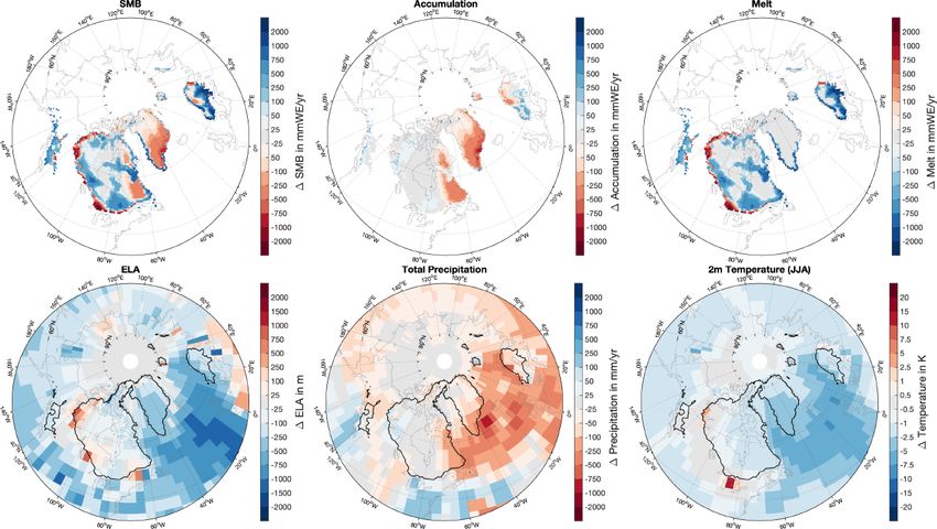
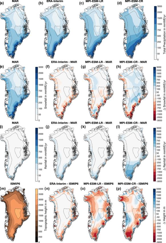
M.-L. Kapsch et al.: Surface mass balance changes throughout the last deglaciation                                                1139

Figure 2. (a–d) Total Precipitation as simulated by (a) MAR, (b) ERA-Interim, (c) MPI-ESM-LR, and (d) MPI-ESM-CR for 1980–2010.
(e–h) Snowfall and (i–l) rainfall in (e, i) MAR and differences between (f, j) ERA-Interim, (g, k) MPI-ESM-LR, and (h, l) MPI-ESM-CR and
MAR. (m–p) Topography from (m) ISMIP6 and the differences in topography between ISMIP6 and (n) ERA-Interim, (o) MPI-ESM-CR,
and (p) MPI-ESM-LR. Note that the values are bi-linearly interpolated onto the ISMIP6 topography from the original model data, not the
downscaled values. Black contours mark surface elevations of 0, 1000, 2000, and 3000 m.

https://doi.org/10.5194/tc-15-1131-2021                                                      The Cryosphere, 15, 1131–1156, 2021
1140                                   M.-L. Kapsch et al.: Surface mass balance changes throughout the last deglaciation

EBMERAI , EBMMPI-ESM-CR , and EBMMPI-ESM-LR simulate               3.2    Melt
lower accumulation than MAR, as well as the Regional At-
mospheric Climate Model (RACMO; Table 3; Noël et al.,              Integrated over the ice sheet, EBMERAI , EBMMPI-ESM-CR ,
2019). This difference is associated with less snowfall and        and EBMMPI-ESM-LR simulate less melt than MAR and
more rainfall in ERA-Interim and the two MPI-ESM simu-             RACMO (Table 3), but the sign of the differences varies sig-
lations than in the regional models, specifically in the low-      nificantly depending on the region (Fig. 1). EBMMPI-ESM-CR
elevation areas along the coastal areas of Greenland (Fig. 2).     shows significantly more surface melt along the western mar-
The underestimation of ERA-Interim’s snowfall that extends         gins of the ice sheet than MAR (Fig. 1). These areas are
into the high-elevation areas of the ice sheet is likely as-       topographically higher in MPI-ESM-CR than the ISMIP6
sociated with an unrealistic representation of clouds and a        topography (Fig. 2). One problem of downscaling melt in
low cloud bias, as well as shortcomings in modeling sea-           these regions is that temperatures are always at the freez-
sonal changes in surface temperatures (see Sect. 3.2; Miller       ing point during melting. By projecting the temperatures
et al., 2018). In the higher-elevation areas of most of the        onto lower elevations, the height-corrected temperatures de-
central parts of Greenland, MPI-ESM-CR and MPI-ESM-                part significantly from the freezing point towards higher tem-
LR overestimate snowfall, which is tightly linked to to-           peratures. Hence, the vertical downscaling from higher el-
pographic differences underlying the models, as well as            evations to low elevations overestimates melting. In con-
model biases in the atmospheric circulation patterns affect-       trast, the area in the south that is significantly higher than
ing precipitation (Fig. 2; Mauritsen et al., 2019). Areas that     the ISMIP6 topography shows less melt. It indicates that
are lower in MPI-ESM-CR and MPI-ESM-LR than MAR,                   most of the differences are closely related to differences in
mainly due to the spectral smoothing in MPI-ESM, generally         the topography. Comparisons with EBMMPI-ESM-LR , which
show more snowfall in the MPI-ESM simulations (Fig. 2).            shows less melt in the north and west of the ice sheet com-
Comparing the accumulation derived from EBMMPI-ESM-CR              pared to EBMMPI-ESM-CR (Figs. 1 and 2), confirm that dif-
with EBMMPI-ESM-LR shows that accumulation patterns in             ferences in the melt patterns are linked to the underlying to-
the southeast of the ice sheet are more confined towards           pographies of the model versions. MPI-ESM-LR is slightly
the east coast, but EBMMPI-ESM-LR still presents a signif-         higher than MPI-ESM-CR and thereby closer to MAR on
icant underestimation of accumulation in the low-elevation         the northern and western flanks of the ice sheet; hence,
areas. Hence, even the higher resolution of MPI-ESM-LR is          EBMMPI-ESM-LR shows less melt than EBMMPI-ESM-CR in
not sufficient to represent the regionally confined processes      these areas. EBMERAI shows less melt in the southern and
that determine the accumulation in these regions. The over-        western parts of the ice sheets than MAR. These low melt
estimation of accumulation in the north of the ice sheet is        rates are partly a result of the model tuning towards a similar
reduced in EBMMPI-ESM-LR compared to EBMMPI-ESM-CR .               integrated Greenland SMB value (see Table 3).
The reduction is likely associated with a better representa-          Heat fluxes towards the surface control predominately sur-
tion of the topographic gradients in the MPI-ESM-LR ver-           face temperatures and melting. Miller et al. (2018), who com-
sion of the model and an associated shift in precipitation         pared surface energy fluxes over Greenland from different re-
patterns reducing precipitation at higher elevation. The com-      analyses with surface observations, found that ERA-Interim
parison between EBMMPI-ESM-LR and EBMMPI-ESM-CR indi-              largely underestimates downward longwave and shortwave
cates that an increase in resolution should not always resolve     radiation, which is likely associated with an unrealistic repre-
all biases. This is in line with findings by van Kampenhout        sentation of cloud optical properties. Low surface albedos in
et al. (2019) showing that a regional grid refinement in sim-      ERA-Interim and an associated underestimation of outgoing
ulations with the Community Earth System Model (CESM)              shortwave radiation partially compensate for the downward
did not improve all SMB components. Model biases, e.g., in         longwave radiation deficit. Further, seasonal biases in the la-
the large-scale circulation, clouds, and precipitation patterns    tent heat fluxes dampen the seasonal changes in surface tem-
(Mauritsen et al., 2019), as well as uncertainties due to inter-   peratures. Such biases are not unique to ERA-Interim but can
nal variability, are exhibited in all ESMs and explain part of     also be found in other reanalyses (for details see Miller et al.,
the differences seen in the presented comparison.                  2018) and models, such as MAR (Fettweis et al., 2017). We
   Note that the EBM calculates snowfall as precipitation at       find similar biases in the EBMMPI-ESM-LR simulation which
temperatures below 0 ◦ C and partly compensates for these          are likely associated with the simulated cloud cover.
differences in snowfall and rainfall specifically along the
coastal areas in the west and southeast of the ice sheet
(not shown). The seasonal differences are larger. In summer,       4     SMB and ELA changes throughout the last
ERA-Interim simulates less snowfall and more rainfall but                deglaciation
shows slightly less total precipitation than MAR, which im-
pacts the melt patterns (not shown).                               The evaluation shows that major differences between MAR
                                                                   and EBMMPI-ESM-CR are the increased melt on the west-
                                                                   ern flank of Greenland and along the coastal areas, as well

The Cryosphere, 15, 1131–1156, 2021                                                    https://doi.org/10.5194/tc-15-1131-2021
M.-L. Kapsch et al.: Surface mass balance changes throughout the last deglaciation 1141
as the overestimation in accumulation in the southern part temperatures that exceed the freezing point in these areas
of Greenland. The latter can partly be reduced by increas- and lead to enhanced melt during summer. In the other ar-
ing the model resolution, as shown by comparisons with eas over Greenland, temperatures are, despite warmer sum-
EBMMPI-ESM-LR . Given these model limitations, the SMB mers, still too cold to trigger melt. As the increase in accu-
is modeled well in comparison to MAR (or other regional mulation dominates enhanced melting, the SMB time series
models; see also Fettweis et al., 2020) with the advantage of increases until about 15 ka (Figs. 3 and 4). Interestingly, the
reduced computational costs that allow for a thorough inves- ELA increases despite an SMB increase. Per definition, the
tigation of the SMB for long-term climate simulations. ELA depends directly on shifts in areas of net melt and ac-
In the following, we present the climate of the deglaciation cumulation. Hence, it closely follows the increase in the ab-
experiment with MPI-ESM-CR based on GLAC-1D bound- lation area. From the LGM to 15 ka, the area of net ablation
ary conditions. We limit the analysis to the Northern Hemi- increases from 0 to about 58 400 km2 .
sphere ice sheets only, with a specific focus on Greenland. A simultaneous increase in SMB and ELA seems to be
counterintuitive at first given that in a present-day climate,
4.1 Greenland a decrease in SMB over Greenland is associated with an in-
crease in the ELA and vice versa (e.g., Le clec’h et al., 2019).
As the SMB is highly dependent on the prescribed ice-sheet As the climate warms, the area of net ablation expands, while
geometry, it is challenging to interpret SMB changes for ice the area of net accumulation recedes, which moves the ELA
sheets that undergo substantial geometry changes throughout upward. As melt is close to zero in the glacial climate, the
the deglaciation. As all Northern Hemisphere ice sheets ex- SMB is dominated by the significant growth of accumulation
cept Greenland disappear entirely, we investigate the SMB due to warmer atmospheric temperatures and the associated
evolution mainly for Greenland, where changes in the geom- increase in precipitation. The dominance of the accumulation
etry were relatively small (Fig. 3, gray line in the top panel). in controlling the SMB explains the counterintuitive behav-
Values for the SMB, ELA, accumulation, and melt integrated ior of the SMB and ELA in the glacial climate. Further, it
over Greenland are shown in Fig. 3. The SMB and ELA for suggests that changes in the ELA cannot be taken as a proxy
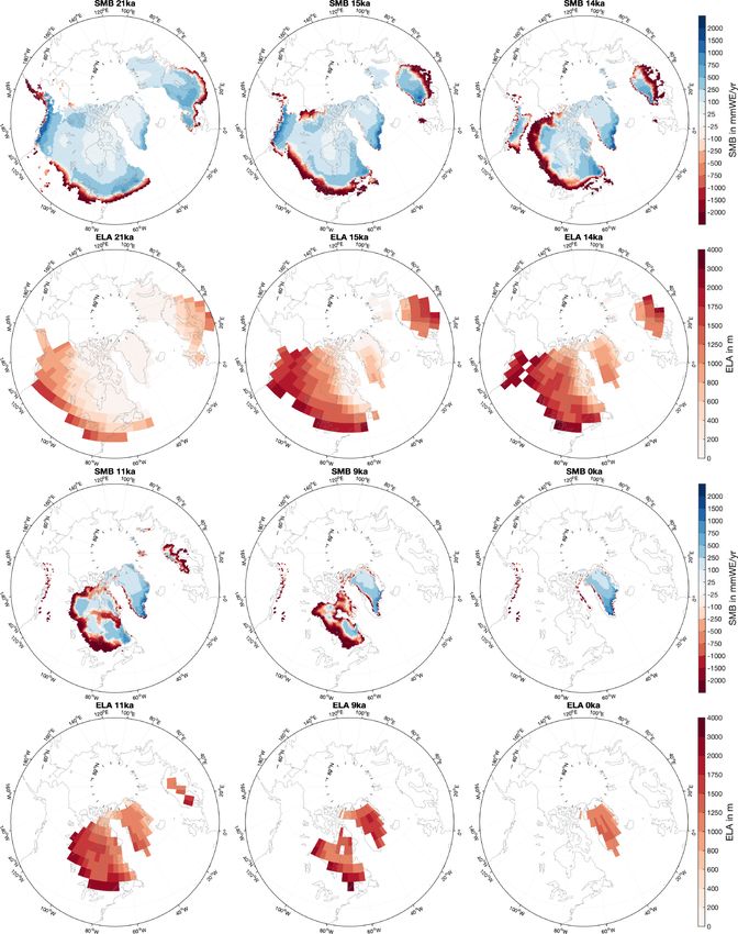
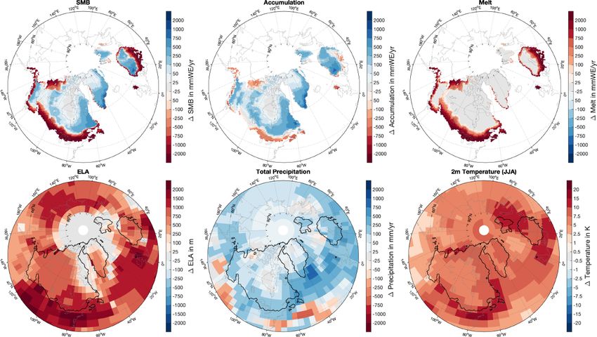
six time slices of the deglaciation are shown in Fig. 4 in order for changes in the SMB.
to indicate the most drastic changes in the Northern Hemi- At around 14.6 ka, the SMB and ELA over Greenland de-
sphere ice-sheet configuration. crease significantly for about 500 years, the SMB drops from
Cold Northern Hemisphere temperatures during the Last about 630 to 380 Gt a−1 , and the ELA decreases from more
Glacial Maximum (LGM; approx. 21 to 19 ka) are associ- than 460 to 120 m (Fig. 3). Regionally, differences are even
ated with a positive Greenland-wide integrated SMB of about larger (Fig. 6). These drastic changes are associated with
380 Gt a−1 . This SMB is dominated by accumulation, while a significant reduction in the AMOC as a response to in-
melt is close to zero (Figs. 3 and 4). This result is consis- creased inflow of freshwater from melting ice sheets into
tent with the Greenland ice sheet being close to its maxi- the global ocean, as prescribed from the GLAC-1D ice-sheet
mum extent during this period (Clark et al., 2009). Due to the reconstructions. The strong meltwater pulse leads to a near
increase in temperatures following an increase in Northern shutdown of the thermohaline circulation and a significant
Hemisphere summer insolation by approximately 7 % of the cooling of the North Atlantic and adjacent regions (Fig. 6).
LGM value and a simultaneous increase in the global CO2 Although the largest cooling is occurring over the North At-
concentrations from 187 ppmv (parts per million by volume) lantic, the annual cooling signal extends over large regions
at 19 ka to 228 ppmv at 15 ka, both accumulation and melt of the Northern Hemisphere, including the Arctic Ocean, the
increase. The total accumulation over Greenland increases North Pacific, and large parts of Eurasia and North Amer-
from about 420 Gt a−1 at 19 ka to about 670 Gt a−1 at 15 ka ica (Fig. 6). Over Greenland, this cooling diminishes surface
(more than 35 %). The largest accumulation increase is ev- melt during summer, which is similar to LGM conditions.
ident over the southwestern part of the ice sheets, which is Again, the largest response is evident over the low-elevation
associated with more precipitation (Fig. 5). Intriguingly, the areas along the southern coasts of Greenland (see also Fig. 5
increase in precipitation is not a uniform signal for the entire for similarities). Associated with the overall cooling is a de-
Northern Hemisphere but shows regional patterns, such as a cline in precipitation which reduces accumulation by more
decrease over parts of the North Atlantic and south of the than 40 % over the ice sheet. Although melt and accumu-
Laurentide ice sheet edge. These patterns indicate that pre- lation again partly compensate for each other, accumulation
cipitation changes are not entirely thermodynamically driven changes occur over a much larger area and dominate changes
(the atmosphere being able to hold more water with increas- in melt so that the integrated SMB decreases for Greenland
ing temperatures) but points towards changes in the atmo- (Fig. 3).
spheric dynamics. Melt increases from about 0 to 25 Gt a−1 After the recovery of the AMOC at around 14 ka, the SMB
between the LGM and 15 ka. The growing melt is small and declines, and the ELA continues to move upward. It thereby
limited to the low-elevation areas along the coast of Green- follows the overall warming signal as a response to increas-
land. This growth is a consequence of increasing summer ing insolation and atmospheric greenhouse gases (Figs. 3 and
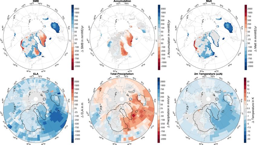
https://doi.org/10.5194/tc-15-1131-2021 The Cryosphere, 15, 1131–1156, 20211142 M.-L. Kapsch et al.: Surface mass balance changes throughout the last deglaciation Figure 3. (a) Greenland SMB, accumulation, melt, and ice-sheet area and (b) equilibrium line altitude (ELA) and meridional overturning circulation (MOC) for the EBMMPI-ESM-CR experiment, together with summer insolation at 65◦ N and CO2 concentration throughout the last deglaciation (21 to 0 ka). Here, 0 ka refers to the year 1950. SMB, accumulation, melt, and ELA (dashed) are integrated over the glacial mask of each individual 100-year time slice. Additionally, the ELA (solid) is integrated over the constant 21 ka ice-sheet mask in order to investigate differences due to the ice-sheet mask. The MOC is the overturning strength at 30.5◦ N at a depth of 1023 m, as in Klockmann et al. (2016). The CO2 concentration is taken from Köhler et al. (2017) and the summer insolation from Berger and Loutre (1991). 4). The decline in the SMB is associated with an overcom- sequently, the ELA decreases, and the SMB begins to recover pensation of the accumulation by a significant increase in continuously after about 8.7 ka. Note that a series of smaller melting. Thus, ELA and SMB are anticorrelated from about AMOC weakening events is evident at around 10.1, 8.4, and 14 ka onward and continue to increase and decrease, respec- 7.1 ka, but their climate impact on the ELA and SMB does tively. Only at around 13.6 and 11.6 ka do the ELA and SMB not manifest significantly in the time series for Greenland decrease significantly again due to a second and third weak- (Fig. 3). The ELA decrease and SMB increase continue until ening of the AMOC. Similar to the first AMOC decline, 200 years BP despite a slight increase in the CO2 concentra- the associated cooling of the North Atlantic and parts of tion. These continuing changes suggest that the decreasing Greenland leads to a decrease in accumulation, melt, and the summer insolation drives SMB and ELA changes between ELA (Fig. 7). The changes are regionally very similar to the 9 ka and 200 years BP. It is not before 100 years BP that first event (Fig. 6). However, the Greenland integrated SMB the ELA and SMB closely follow the CO2 signal again. The shows a weaker signal in both cases than during the first sharp drop in the SMB and the uplift of the ELA for the freshwater event as the changes in accumulation and melt last 100 years of the simulation is similar to the warm pe- partly compensate for each other when integrated over the riod observed in the coastal temperatures of Greenland in the ice sheet (Fig. 3). 1930s (Chylek et al., 2006). At the end of the simulation, After the two AMOC events, the retreat of the Greenland the ELA lies at about 1150 m, and the SMB reaches values ice sheet towards its present-day state continues and is as- of 550 Gt a−1 . These values are similar to values observed sociated with a decrease in SMB and an increase in ELA. during the 21st century, although they are slightly higher as The minimum SMB (216 Gt a−1 ) is reached at 8.7 ka, and no anthropogenic forcings are considered in the deglaciation the maximum ELA (1556 m) occurs at 9.3 ka (Figs. 3 and 4), simulation (see Fig. 4, Sect. 3 and Table 3; Box, 2013). corresponding to the Holocene Thermal Maximum (for a re- The SMB and ELA derived from the MPI-ESM-CR simu- cent review, see Axford et al., 2021). Due to the continuing lation with the prescribed ICE-6G ice sheets are qualitatively deglaciation, Greenland experiences its largest ice volume similar to the presented results based on the GLAC-1D ice- and extent changes between 10.8 and 9.1 ka (the ice-sheet ge- sheet reconstructions (see Figs. A2 to A6). The overall trends ometry influences SMB values during this period). At around of both variables, as well as the relationships between accu- 11.1 ka, the Northern Hemisphere summer insolation reaches mulation and melt (e.g., accumulation dominating melting its maximum and decreases continuously thereafter until the until about 15 ka), are similar, but the timing of the weaken- present, while the CO2 concentration remains rather constant ing of the AMOC, as well as the magnitude, differs. These between 11.1 and 6 ka and slightly increases thereafter. Con- deviations are due to a different timing, magnitude, and lo- The Cryosphere, 15, 1131–1156, 2021 https://doi.org/10.5194/tc-15-1131-2021
You can also read