How catchment characteristics influence hydrological pathways and travel times in a boreal landscape - HESS
←
→
Page content transcription
If your browser does not render page correctly, please read the page content below
Hydrol. Earth Syst. Sci., 25, 2133–2158, 2021
https://doi.org/10.5194/hess-25-2133-2021
© Author(s) 2021. This work is distributed under
the Creative Commons Attribution 4.0 License.

How catchment characteristics influence hydrological pathways and
travel times in a boreal landscape
Elin Jutebring Sterte1,2 , Fredrik Lidman1 , Emma Lindborg2 , Ylva Sjöberg3 , and Hjalmar Laudon1
1 Department  of Forest Ecology and Management, Swedish University of Agricultural Sciences, 901 83 Umeå, Sweden
2 DHI Sweden AB, Skeppsbron 28, 111 30 Stockholm, Sweden
3 Center for Permafrost (CENPERM), Department of Geosciences and Natural Resource Management, University of

Copenhagen, Øster Voldgade 10, 1350 Copenhagen, Denmark

Correspondence: Elin Jutebring Sterte (eljs@dhigroup.com)

Received: 13 March 2020 – Discussion started: 1 April 2020
Revised: 5 March 2021 – Accepted: 15 March 2021 – Published: 20 April 2021

Abstract. Understanding travel times and hydrological path-       during the snowmelt period. However, this lower groundwa-
ways of rain and snowmelt water transported through the           ter recharge during snowmelt caused mire-dominated catch-
landscape to recipient surface waters is critical in many hy-     ments to have longer stream runoff MTTgeo than comparable
drological and biogeochemical investigations. In this study,      forest catchments in winter. Boreal landscapes are sensitive
a particle-tracking model approach in Mike SHE was used           to climate change, and our results suggest that changes in
to investigate the pathway and its associated travel time of      seasonality are likely to cause contrasting responses in differ-
water in 14 partly nested, long-term monitored boreal sub-        ent catchments depending on the dominating landscape type.
catchments of the Krycklan catchment (0.12–68 km2 ). This
region is characterized by long and snow-rich winters with
little groundwater recharge and highly dynamic runoff during
spring snowmelt. The geometric mean of the annual travel          1   Introduction
time distribution (MTTgeo ) for the studied sub-catchments
varied from 0.8 to 2.7 years. The variations were related to      The pathways and associated travel times of water through
the different landscape types and their varying hydrological      the terrestrial landscape to stream networks is a widely dis-
responses during different seasons. Winter MTTgeo ranged          cussed topic in contemporary hydrology. This interest has
from 1.2 to 7.7 years, while spring MTTgeo varied from            emerged because of the significant role travel time and rout-
0.5 to 1.9 years. The modelled variation in annual and sea-       ing of water through various subsurface environments play in
sonal MTTgeo and the fraction of young water (
2134                           E. Jutebring Sterte et al.: How catchment characteristics influence hydrological pathways

ity, and seasonality (Botter et al., 2010; Lin, 2010; Heid-       plementary stories about the specific pathways water takes
büchel et al., 2012; Hrachowitz et al., 2013). Therefore, es-     from the source to the recipient stream (Laudon et al., 2011).
timating travel times for contrasting landscape elements is          A complementary approach to field experiments is numer-
challenging, but when successful, it will enhance our ability     ical modelling, which can help achieve a more complete sys-
to understand and predict catchment functioning more ade-         tem understanding. Lumped hydrological models often de-
quately.                                                          scribe catchments as single integrated entities. In contrast,
   Stream water consists of a blend of overland flow and          distributed numerical models can include spatial heterogene-
groundwater of different ages. The mean travel time (MTT)         ity in input parameters and therefore have the potential to
to streams is calculated as the average age of this mix           represent catchment processes more mechanistically. In turn,
(McGuire and McDonnell, 2006). The baseflow is the part           this can lead to a more process-based understanding of hy-
of stream groundwater contribution that generally has trav-       drology and biogeochemistry at the catchment scale (Brirhet
elled the furthest and is the oldest (Klaus et al., 2013; Hra-    and Benaabidate, 2016; Soltani, 2017). Common methods to
chowitz et al., 2016). In contrast, young stream water is typi-   calculate travel times using numerical methods include mod-
cally connected to overland flow or shallow subsurface path-      els using solute transport routines and particle tracking (Hra-
ways, which mainly can be seen at times with large rain           chowitz et al., 2013; Ameli et al., 2016; Kaandorp et al.,
or snowmelt inputs (Peters et al., 2014; Hrachowitz et al.,       2018; Remondi et al., 2018; Yang et al., 2018; Heidbüchel
2016). The variability of water sources makes the travel time     et al., 2020). Models, however, need – as far as possible –
distribution difficult to quantify, especially on intra-annual    proper tests against empirical observations to build confi-
timescales, as they vary in time and space depending on           dence in their output. Stream discharge, groundwater levels,
numerous scale-dependent and scale-independent processes          and tracer data are examples of such validation data that can
(Botter et al., 2010). A better understanding of the seasonal     provide vital information (McGuire et al., 2007; Hrachowitz
variability in the fraction of young and old waters can help      et al., 2015; Wang et al., 2017). The collection of such field
provide insights into the fundamental role catchment charac-      data is, however, costly and time-consuming. Therefore, data
teristics play in regulating the hydrology and biogeochem-        for calibration and validation are often limited, and the min-
istry of streams and rivers.                                      imum length and types in data-sparse catchments are cur-
   Stable water isotopes and biogeochemical tracers are com-      rently a topic of increasing interest (Bjerklie et al., 2003; Jian
mon tools applied in field investigations to locate water         et al., 2017; Li et al., 2018).
sources and follow their pathways through the landscape              Snow-dominated landscapes have received increasing at-
(Maulé and Stein, 1990; Rodhe et al., 1996; Goller et al.,        tention in the last decades due to their importance as wa-
2005; Tetzlaff and Soulsby, 2008). Isotopic tracer signal         ter resources (Barnett et al., 2005) and their vulnerability to
dampening can provide an estimate of MTT (Uhlenbrook et           climate change (Tremblay et al., 2011; Aubin et al., 2018).
al., 2002; McGuire et al., 2005; Peralta-Tapia et al., 2016),     Landscapes with long-lasting snow cover that often melts
and more elaborate time-series analysis can offer quantitative    rapidly in the spring create both opportunities and challenges
assessments of travel times (Harman, 2015; Danesh-Yazdi et        for determining the pathways and travel time of water dis-
al., 2016). However, the isotope amplitude signal used to es-     charging to streams. The long, snow-rich winters not only
timate MTT in many transfer functions is lost after approx-       cause protracted periods of winter baseflow with little or no
imately 4 to 5 years because of effective mixing (Kirchner,       recharge (Spence et al., 2011; Spence and Phillips, 2015;
2016), limiting the use of isotopes in catchments with long       Lyon et al., 2018), but they also cause considerable amounts
travel times. The young water fraction, often defined as water    of water during the often short and intensive snowmelt in
younger than 2 to 3 months, can, however, still be quantifi-      the spring. Although attempts to assess travel times gener-
able in such catchments (von Freyberg et al., 2018; Lutz et       ally have provided useful results using, for example, models
al., 2018; Stockinger et al., 2019). The main advantage of wa-    to reconstruct isotope signal dampening in snow-dominated
ter isotopes is that they are relatively conservative and frac-   catchments, the winter season has proven to be especially
tionate primarily because of evaporation. Hence, once in the      challenging, suggesting that other methods to assess travel
subsurface environment, the signal is only affected by mix-       times may be required (Heidbüchel et al., 2012; Peralta-Tapia
ing different water sources. In contrast, many biogeochemi-       et al., 2016). The boreal region also consists of numerous
cal tracers react and transform on their route to streams (Lid-   patches of lakes and mires, interspersed in a landscape dom-
man et al., 2017; Ledesma et al., 2018). Such transformation      inated by coniferous forests on different soil types, which
and reactions depend on the specific solute and soil environ-     makes this task even more challenging. Hence, accounting
ment that water encounters and, therefore, give qualitative       for the unique circumstances of both baseflow with long
information about groundwater flow pathways (Wolock et            travel times and those of the intensive spring snowmelt with
al., 1997; Frisbee et al., 2011; Zimmer et al., 2012). Com-       potential large overland flow components in heterogeneous
bined information from conservative and reactive tracers can      landscapes requires models that can handle the complexity
hence provide an enhanced understanding of hydrological           and separation of various flow components across scales, soil
processes as their concentrations and dynamics can tell com-      types, and landscape patches.

Hydrol. Earth Syst. Sci., 25, 2133–2158, 2021                                      https://doi.org/10.5194/hess-25-2133-2021
E. Jutebring Sterte et al.: How catchment characteristics influence hydrological pathways                                   2135

   To overcome previous limitations, this study used parti-       2     Method
cle tracking in the physically based distributed numerical
model, Mike SHE (Graham and Butts, 2005), to enhance our          2.1    Site description
understanding of stream water contribution in boreal land-
scapes across seasons and landscape configurations. The wa-       The Krycklan study catchment, located in the boreal region
ter movement model in Mike SHE calculates saturated (3D)          at the transition of the temperate/subarctic climate zone of
groundwater flow and unsaturated (1D) flow and is fully in-       northern Sweden, spans elevations from 114 to 405 m a.s.l.
tegrated with the surface water and evapotranspiration. The       (Fig. 1, Table 1). The characteristic vegetation of this boreal
water flow model setup and results previously presented by        landscape is the dominance of Scots pine (Pinus sylvestris)
Jutebring Sterte et al. (2018) were used as the study platform    and Norway spruce (Picea abies), covering most of the
for this work. The model has been calibrated and validated        catchment (Laudon et al., 2013). In this study, we refer to
to 14 sub-catchments using daily stream-discharge observa-        soil as all unconsolidated material above the bedrock.
tions and periodical measured groundwater levels in 15 wells          Krycklan has a landscape distinctively formed by the last
throughout the Krycklan catchment in the boreal region of         ice age (Ivarsson and Johnsson, 1988; Lidman et al., 2016).
northern Sweden (Laudon et al., 2013; Jutebring Sterte et al.,    At the higher elevations to the north-west, located above the
2018). The model complexity allows for an in-depth inves-         highest postglacial coastline, the soils can reach up to 15–
tigation of advective travel times by non-reactive particle-      20 m in thickness. Here, the soil primarily consists of glacial
tracking simulations in a transient flow field.                   till, and the landscape is intertwined with lakes and peat-
   The main objective of this study was to quantify annual        lands. The deeper soils consist of basal till which was de-
and seasonal (winter, spring, and summer) travel time dis-        posited and compacted under the moving ice. In contrast, the
tributions and calculate MTT of water runoff to streams of        shallower till layers consist primarily of ablation till, which
the Krycklan sub-catchments to disentangle how these are          is less compact since it mainly has been compacted by its
related to physical landscape characteristics and variation in    own weight (Goldthwait, 1971). This causes a decreasing hy-
groundwater recharge. Firstly, the credibility of the model       draulic conductivity with depth, which is characteristic for
results was tested by comparing calculated travel times for       glacial till in northern Sweden (Bishop et al., 2011; Nyberg,
the 14 sub-catchments to 10-year observational records from       1995; Seibert et al., 2009). At lower elevations, the soils con-
Krycklan, including average seasonal changes in stream iso-       sist of fluvial and glaciofluvial deposits of primarily sandy
tope signatures and base cation concentrations. The useful-       and silty sediments. Compared to the soil at higher eleva-
ness of stream isotopic composition and chemistry record          tions in the catchment, these deposits can reach thicknesses
has previously been demonstrated for understanding the con-       up to approximately 40 to 50 m and have a hydrological con-
nection of hydrological flow pathways and travel times for        ductivity that is more constant with depth because these soil
this site (Laudon et al., 2007; Peralta-Tapia et al., 2015) but   types have mainly been compacted only by their own weight.
with the limitation of studies on only short periods or sin-          For more than 30 years, multi-disciplinary biogeochemi-
gle catchments. Secondly, the purpose was to go beyond            cal and hydrological studies have been conducted in Kryck-
what was previously done by identifying the connection be-        lan (e.g. Laudon and Sponseller, 2018). Streamflow is moni-
tween travel times and different catchment characteristics        tored in 14 nested sub-catchments, called C1 to C20, with the
and test how this varies depending on the hydrological con-       longest continuously monitored time series starting at the be-
ditions. This was accomplished by capturing contrasting sea-      ginning of the 1980s. Connected by a network of streams, the
sons such as the low-flow conditions in winter with limited       different sub-catchments allow an evaluation of the effects of
input of new precipitation, high flow in spring when the sys-     catchment characteristics on hydrologic transport, including
tem is still partly frozen, and summer when evapotranspira-       soil type, vegetation, and differences in topography (Table 1).
tion (ET) becomes a significant process. We focused espe-
cially on the catchment characteristics that have been sug-       2.2    Linking seasonal base cation concentration and
gested to be important factors for regulating stream chem-               isotopic signature to travel times to stream water
istry of the Krycklan sub-catchments, including the areal
coverage of mires, catchment size, soil properties, and sea-      This study was focused on three seasons in Krycklan: winter,
sonal changes in groundwater recharge (Karlsen et al., 2016;      spring, and summer (Tables 2, A1, Appendix). For evaluation
Klaminder et al., 2011; Laudon et al., 2007; Peralta-Tapia et     of stream chemistry, we defined the winter as late early De-
al., 2015; Tiwari et al., 2017).                                  cember to late February, from the time air temperatures were
                                                                  below 0 ◦ C, until the air temperature started to rise above
                                                                  freezing temperatures again, causing snowmelt. This season
                                                                  is characterized by an extensive and permanent snow cover
                                                                  with little or no groundwater recharge. We assumed that the
                                                                  winter stream composition reflects the chemistry of deeper
                                                                  groundwater (Fig. 2). Similarly, we defined spring as the hy-

https://doi.org/10.5194/hess-25-2133-2021                                        Hydrol. Earth Syst. Sci., 25, 2133–2158, 2021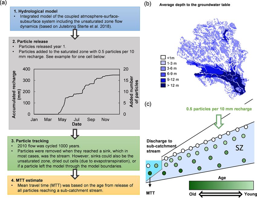
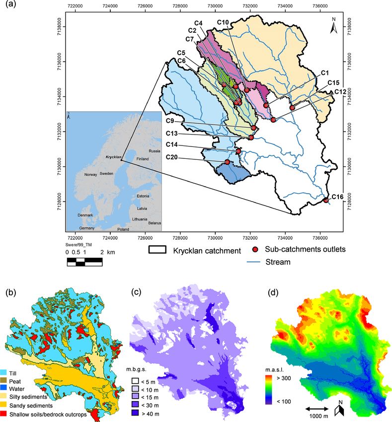
2136                              E. Jutebring Sterte et al.: How catchment characteristics influence hydrological pathways

Figure 1. The Krycklan catchment. (a) Locations of sub-catchments and their outlets. The areas are colour-coded based on their stream
network connections; e.g. all sub-catchments of one colour connect before reaching the white area. For further details of the catchment
characteristics, see Table 1. (b) The figure shows the soil map used in the Mike SHE flow model, which is based on data from the Swedish
Geological Survey soil map (1 : 100 000) and field investigations. (c) Soil depth to bedrock map taken from the Swedish Geological Sur-
vey (2016) and is shown in metres below the ground surface (m b.g.s.). (d) Catchment topography, shown as metres above sea level (m a.s.l.).

drological period directly influenced by the snowmelt. The              months between the three distinct seasons. This is because
main part of the snowmelt and spring flood occurs in April–             snowmelt influences runoff in March and June. October and
May. During snowmelt, ca. 50 % of the annual precipitation              November are transitional months between summer and win-
leaves the system in a short period of time, diluting base-             ter conditions, with irregularly occurring snowfall and soil
flow with new input of water. Finally, we defined the summer            frost events.
season as the period between July and September when the                   In this study, stable water isotopes (δ 18 O) were used to
hydrology is characterized by rain, high ET, and relatively             track pathways of precipitation inputs to stream networks
little runoff. March, June, October, and November were ex-              (see the Appendix for the δ 18 O definition). Ten years of
cluded because, hydrologically, they are typically transition           δ 18 O measurements for 13 of the 14 sub-catchments were

Hydrol. Earth Syst. Sci., 25, 2133–2158, 2021                                             https://doi.org/10.5194/hess-25-2133-2021
E. Jutebring Sterte et al.: How catchment characteristics influence hydrological pathways                                                                                              2137

Table 1. Sub-catchment characteristics. The list includes all 14 monitored sub-catchments in Krycklan, called C1 to C20, including the entire
Krycklan catchment, C16. Different branches of the stream network are gathered in the table and illustrated in distinct colours in Fig. 1. The
table includes the sub-catchment area, average elevation, and average slope. Further descriptions of these characteristics can be found in
Karlsen et al. (2016). The table also includes soil proportion based on the soil map (1 : 100 000) from the Swedish Geological Survey (2016).

                       Catchment size              Average elevation               Slope         Till      Mire        Sandy sediments               Silty sediments          Lake
                              (km2 )                       (m a.s.l.)                 (◦ )      ( %)       ( %)                   ( %)                          ( %)           ( %)
            C2                         0.12                             273          4.75         79            0                             0                           0    0.0
            C4                         0.18                             287          4.24         29           42                             0                           0    0.0
            C5                         0.65                             292          2.91         47           46                             0                           0    6.4
            C6                         1.10                             283          4.53         51           29                             0                           0    3.8
            C7                         0.47                             275          4.98         68           16                             0                           0    0.0
            C9                         2.88                             251          4.25         64           14                             7                           4    1.5
            C13                        7.00                             251          4.52         60           10                             9                           9    0.7
            C1                         0.48                             279          4.87         91            0                             0                           0    0.0
            C10                        3.36                             296          5.11         64           28                             1                           0    0.0
            C12                        5.44                             277          4.90         70           18                             6                           0    0.0
            C14                       14.10                             228          6.35         46            6                            24                          15    0.7
            C20                        1.45                             214          5.96         55            9                             0                          28    0.0
            C15                       19.13                             277          6.38         64           15                             8                           2    2.4
            C16                       67.90                             239          6.35         51            9                            21                          10    1.0

Table 2. Seasonal stream chemistry. The table includes average winter signatures (‰) and the average difference between annual winter–
spring and winter–summer signatures (1δ 18 O). The table also includes average winter, spring, and summer BC concentrations.

                                                          δ 18 Oa                                                                      Base cations (BC)b
                             Winter                      Spring                       Summer                     Winter                     Spring                     Summer
                                                                                                              concentration              concentration               concentration
                         ‰      SD/SEMc          1δ 18 O       SD/SEM          1δ 18 O       SD/SEM         µeq/L SD/SEM               µeq/L SD/SEM                µeq/L SD/SEM
          C2        −12.9        0.46/0.07        −0.68       0.52/0.16           0.15       0.45/0.16         264          99/20         189           43/6         267        58/9
          C4        −13.1        0.36/0.06        −1.08       0.66/0.20           0.82       0.48/0.21         263          71/16         120           48/8         306       77/12
          C5        −13.0        0.47/0.08        −1.80       0.66/0.20           0.72       0.65/0.21         267          67/16         202           59/8         231        34/5
          C6        −13.1        0.35/0.06        −1.27       0.55/0.16           0.52       0.47/0.17         321          61/12         233         104/14         322      120/16
          C7        −13.0        0.22/0.04        −0.73       0.56/0.17           0.42       0.37/0.18         271           40/8         191           57/8         270        38/5
          C9        −13.1        0.29/0.05        −0.98       0.46/0.14           0.57       0.44/0.15         349          57/11         231          73/10         327        61/8
          C13       −13.1        0.26/0.05        −0.83       0.55/0.16           0.60       0.48/0.17         338          57/11         223           50/6         309        43/6
          C1        −12.9        0.28/0.05        −0.53       0.60/0.18           0.10       0.38/0.19         272           36/7         229           44/6         285        31/4
          C10       −13.3        0.28/0.05        −0.80       0.61/0.18           0.53       0.39/0.19         314          50/10         209          82/11         332       72/10
          C12       −13.1        0.30/0.05        −0.88       0.48/0.15           0.36       0.43/0.16         319           43/8         211           58/7         316        45/6
          C14       −13.4        0.23/0.04        −0.70       0.55/0.17           0.48       0.45/0.18         358           34/7         272           69/9         376       74/10
          C20           –                –            –               –              –               –         519          65/13         398         108/14         526        60/8
          C15       −13.4        0.40/0.07        −0.73       0.69/0.21           0.63       0.44/0.22         347           41/8         258           60/8         349        45/6
          C16       −13.4        0.44/0.08        −0.56       0.64/0.64           0.46       0.33/0.20         480          68/13         272           70/9         441       76/10
          Long-term precipitation average – isotopes
          −13.4 ‰d
         a δ 18 O signature (2008–2018); data have been adjusted according to the lake proportion according to Eq. (A7), Appendix.
         b Base cation concentration (2008–2016); data have been adjusted according to the mire proportion.
         c SD: standard deviation; SEM: standard error of the mean.
         d Measured precipitation average for isotopes (2007–2016). The precipitation average is close to equal to isotope measurements of groundwater below ca. 10 m.

https://doi.org/10.5194/hess-25-2133-2021                                                                                  Hydrol. Earth Syst. Sci., 25, 2133–2158, 2021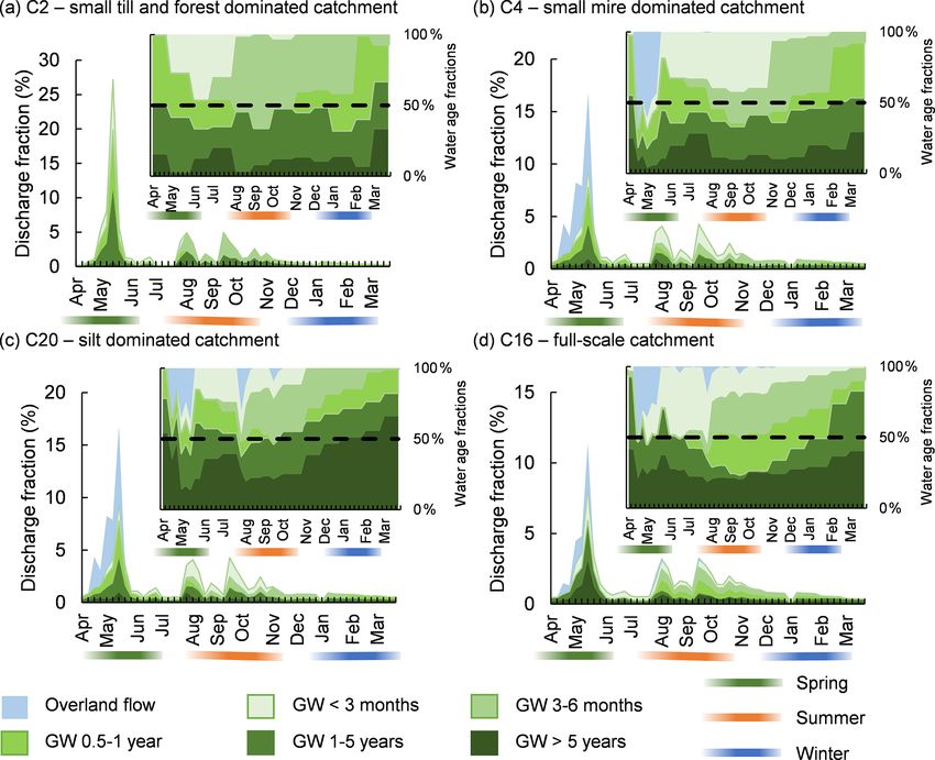
2138 E. Jutebring Sterte et al.: How catchment characteristics influence hydrological pathways
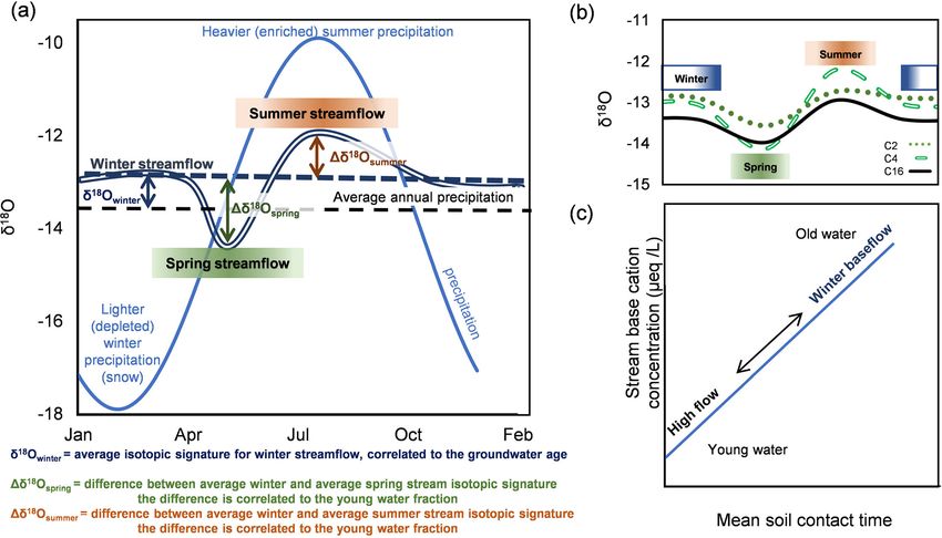
Figure 2. Conceptual figure of travel time to stream vs. stream isotopic signature (a, b) and stream base cation concentration (c). (a)
The connection between δ 18 O and travel time to stream, where the sine curve shows the annual variations of δ 18 O in precipitation, and
approximate seasonal winter, spring, and summer stream compositions are marked and exemplified by the average annual changes in C4.
In winter, the travel times are related to the average deviation in the isotopic signature between the winter baseflow and the long-term
precipitation. In spring, the fraction of young water is correlated with the difference between the average spring stream signature and the
average winter baseflow. In summer, the fraction of young water is correlated with the difference between the average summer stream
signature and average winter baseflow. (b) Seasonal δ 18 O averages for three example streams: C2, C4 and C16. (c) The connection between
base cation (BC) concentration and soil contact time. The longer the water spent in the mineral soil, the higher the stream concentrations of
BCs will be due to soil weathering.
used. Isotopic fractionation caused by lake surface evapora- full mixing of the precipitation signal is reached. The closer
tion affects the isotopic signal of some of the sub-catchments the signature is to the long-term precipitation average (which
(Leach and Laudon, 2019). This fractionation was corrected is equal to the deep groundwater measurements in Kryck-
by accounting for the percentage of lakes in each sub- lan, Laudon et al., 2007), the more well-mixed and, conse-
catchment (Table 2), using the same principle as Peralta- quently, the longer travel times will be found. We used the
Tapia et al. (2015) but adjusted to newly acquired δ 18 O ob- average annual winter signature for the evaluation. In spring,
servations (Eq. A7, Appendix). previous studies have shown that the young water fraction
The comparison of the modelling results to observations can be distinguished by comparing the change in the isotopic
of δ 18 O was based on a conceptual model of the seasonal signature to the preceding winter because the snow is much
variability and differences between precipitation and runoff lighter (depleted in 18 O) (Laudon et al., 2007; Tetzlaff et al.,
(Fig. 2a). The precipitation signal varies on a seasonal ba- 2015). We calculated the difference between the average win-
sis, creating an amplitude difference (Fig 2b). This ampli- ter and average spring signature for all years. The mean dif-
tude is reduced due to groundwater mixing until complete ference we hereafter refer to as the 1δ 18 Ospring , which we
mixing is reached and the groundwater receives the same assumed to be negatively correlated with the young water
signal as the long-term precipitation average. There is no or fraction (Fig. 2a). Similarly, we refer to the mean difference
little groundwater recharge during winter because almost all between annual averages of winter and summer signature as
precipitation inputs arrive and accumulate as snow. Hence, 1δ 18 Osummer , which similarly should be related to the young
we assume that the stream isotopic signature originates from water fraction during the summer. However, in summer, pre-
groundwater only (Laudon et al., 2007; Peralta-Tapia et al., cipitation is heavier (more enriched in 18 O) than in winter,
2015). Consequently, the closer the stream signature comes which hence should give the young water a heavier signal.
to the long-term precipitation average, the more the ground- Therefore, we assumed a positive relationship between the
water has been mixed. The groundwater isotopic signature, in young water fraction and the 1δ 18 Osummer (Fig. 2a).
turn, should be correlated with the travel time to stream until
Hydrol. Earth Syst. Sci., 25, 2133–2158, 2021 https://doi.org/10.5194/hess-25-2133-2021
E. Jutebring Sterte et al.: How catchment characteristics influence hydrological pathways                                   2139

   Another indicator of travel times to stream that we used       cesses. The fully distributed 3D modelling tool uses topogra-
was the sum of base cation (BC) concentration (Fig. 2b)           phy, soil properties, and time-varying climate inputs to cal-
(Abbott et al., 2016). Previous attempts to follow the chem-      culate the water fluxes throughout a catchment (Rahim et al.,
ical development of groundwater in the Krycklan catchment         2012; Sishodia et al., 2017; Wang et al., 2012; Wijesekara
and other streams have shown that the BC concentration in-        et al., 2014). The ET processes include canopy interception,
creases along the groundwater flow pathway (Klaminder et          open surface evaporation, root uptake, sublimation, and soil
al., 2011). Therefore, a correlation between the stream con-      evaporation from the unsaturated zone based on a methodol-
centration of BCs on the one hand and modelled soil con-          ogy developed by Kristensen and Jensen (1975). Flow in the
tact time on the other were assumed in this study. The BCs        saturated zone (SZ) is calculated in 3D by the Darcy equa-
are mainly derived from the weathering of local soils in the      tion. The flow in the unsaturated zone (UZ) is calculated in
Krycklan catchment, with only a minor contribution from at-       vertical 1D using the Richards equation, and overland flow
mospheric deposition (Lidman et al., 2014). Our assumption        (OL) is calculated using a horizontal 2D diffusive wave ap-
is further based on modelling studies of weathering rates in a    proximation in the Saint-Venant equations (Fig. 3). Streams
soil transect in the Krycklan catchment, which indicates that     are modelled in 1D using a high-order dynamic wave formu-
there is a kinetic control of the release of BCs in the soils     lation of the Saint-Venant equations. The river model (Mike
(Erlandsson et al., 2016). Since all BCs behave relatively        11) is not restricted to the grid size of Mike SHE and al-
conservatively in these environments (Ledesma et al., 2013;       lows for a more precise calculation of stream water levels
Lidman et al., 2014), we used their combined concentration        and flow rates. The different model compartments OL, UZ,
as a proxy for soil contact time. However, the assumption is      SZ, and rivers are fully integrated, and water fluxes between
only valid when the water is in contact with mineral soils,       and within the compartments are calculated in each time step
not with peat in mires, which are abundant in some of the in-     of the simulation. More in-depth documentation and manuals
vestigated sub-catchments. There are little minerals present      of Mike SHE and Mike 11 are provided by DHI (DHI, 2021).
in the peat and, therefore, the BC concentration cannot be           For the Krycklan model, the horizontal grid was set to
expected to increase during the time the water spends there.      50 × 50 m. Vertically, the model is divided into 10 calcu-
Therefore, the BC concentrations were adjusted for the influ-     lation layers (CLs) and extends to a depth of 100 m below
ence of mire, using the sub-catchment mire proportion as a        ground. The SZ-CLs vary with depth and are thinner closer
scaling factor to allow a fair comparison to water–soil contact   to the soil surface; the first CLs extend to 2.5, 3, 4, and 5 m,
time (Lidman et al., 2014) (Table 2).                             respectively, below the ground surface, with the soil proper-
   All stream chemistry data come from the online open            ties and depth extension following the stratigraphy (Table 3).
Krycklan database (Table 2) (Krycklan Database, 2013). The        The UZ and SZ interact throughout the soil. If the soil is un-
isotopic signatures contain approximately 10 years of field       saturated, the UZ discretization and equations are used. The
observations (2008 to mid-2018), approximately 25 sam-            influence from ET and UZ processes on the SZ is only fully
ples per year for each site. Parts of the dataset have been       active to the depth of the uppermost SZ-CL. Here, the ET and
published by Peralta-Tapia et al. (2016), where sampling          UZ are calculated at a finer resolution, leading to a detailed
and analyses are described in detail. It has since been ex-       calculation of the groundwater table level. The first SZ-CL
panded using the same methodology. We used the average            depth was set to 2.5 m and was calibrated using the influence
winter isotope signatures from these years as a represen-         of the CL thickness on groundwater table level, UZ, and ET
tation of baseflow. These averages were also compared to          dynamics.
the volume-weighted average of the long-term precipitation,          Following the thickness of the SZ-CL in the Krycklan
calculated using approximately 1000 precipitation measure-        model, all soils above 2.5 m depth are prescribed as one soil
ments of δ 18 O between 2007 and 2016. The precipitation          type, with hydraulic properties being an average of all the
was measured throughout the year, both as rain and as snow.       soil types throughout the vertical profile from the ground sur-
The long-term precipitation average is −13.4 ‰, which is          face to 2.5 m depth. In Mike SHE, horizontal hydraulic con-
close to equal to observations of the isotopic signature at the   ductivity (Kh) is averaged using the thickness of each soil
deep groundwater wells of Krycklan (ca. 10 m depth). The          layer. Vertical flows are more dependent on the lowest ver-
BC data collection methodology is reported in Ledesma et          tical hydraulic conductivity (Kv). Therefore, the harmonic
al. (2013).                                                       weighted mean value is used to calculate the new Kv instead
                                                                  (Table 3). A drain function was used in this model and sev-
2.3   Water flow model setup                                      eral previous studies (Bosson et al., 2012, 2013; Johansson et
                                                                  al., 2015; Jutebring et al., 2018) to account for the higher hy-
We applied the Mike SHE/Mike-11 hydrological modelling            draulic conductivity in the uppermost part of the first CL. In
tools to quantify travel times in a pre-calculated 3D transient   the Krycklan model, the function was activated whenever the
flow field. The simulated terrestrial hydrological system for     groundwater reached 0.5 m below the ground surface, above
the Krycklan catchment includes the saturated and unsatu-         which higher K values have been observed (Table 3) (Bishop
rated flow, ET, snowmelt, overland flow, and streamflow pro-      et al., 2011; Nyberg, 1995; Seibert et al., 2009). The model

https://doi.org/10.5194/hess-25-2133-2021                                      Hydrol. Earth Syst. Sci., 25, 2133–2158, 2021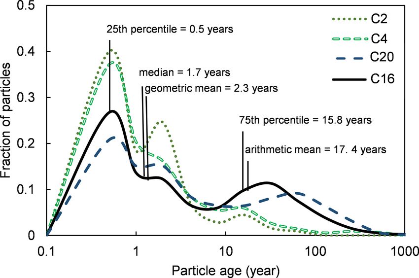
2140                                  E. Jutebring Sterte et al.: How catchment characteristics influence hydrological pathways

Table 3. Flow model setup. Flow model setup from the calibrated and validated Mike SHE model presented in Jutebring Sterte et al. (2018).
The “soil-type surface” corresponds to the soil type shown in Fig. 1b. A drain constant was used to account for coarser material of the upper
half metre of the soil.

                       Soil-type surface          Depth below               Soil type    Horizontal hydraulic           Vertical hydraulic
                                                  ground (m)∗                             conductivity (m/s)            conductivity (m/s)
                       Till                       2.5                       Till                        2 × 10⁻⁵                   2 × 10⁻⁶
                                                  To bedrock                Fine till                   1 × 10⁻⁶                   1 × 10⁻⁷
                                                  Bedrock                                               1 × 10⁻⁹                   1 × 10⁻⁹
                       Peat                       5                         Peat                        1 × 10⁻⁵                   5 × 10⁻⁵
                                                  7                         Clay                        1 × 10⁻⁹                   1 × 10⁻⁹
                                                  To bedrock                Fine till                   1 × 10⁻⁶                   1 × 10⁻⁷
                                                  Bedrock                                               1 × 10⁻⁹                   1 × 10⁻⁹
                       Silty sediments            3                         Silt/clay                   1 × 10⁻⁷                   1 × 10⁻⁷
                                                  To bedrock                Fine till                   1 × 10⁻⁶                   1 × 10⁻⁷
                                                  Bedrock                                               1 × 10⁻⁹                   1 × 10⁻⁹
                       Sandy sediments            4                         Silt/sand                   2 × 10⁻⁵                   2 × 10⁻⁵
                                                  0.9× max depth            Sand                        3 × 10⁻⁴                   3 × 10⁻⁵
                                                  To bedrock                Gravel                      1 × 10⁻⁴                   1 × 10⁻⁴
                                                  Bedrock                                               1 × 10⁻⁹                   1 × 10⁻⁹
                       Drain constant
                       Peat                       1 × 10⁻⁶
                       Till                       4 × 10⁻⁷
                       Silty sediments            1 × 10⁻⁷
                     ∗ The table shows the depth down to which the same description extends. For example, the first description of peat extends
                     down to 5 m, while the first calculation layer is 2.5 m.

also accounted for soil freezing processes, which in Kryck-                             2.4    Establishing travel times – particle tracking
lan have been shown to have a strong influence on the water
turnover in mires (Laudon et al., 2011). Based on a method-                             Particle tracking in Mike SHE enables investigations of
ology presented in Johansson et al. (2015), soil freeze and                             groundwater travel time from the recharge to the SZ until the
thawing processes were described using time-varying K and                               discharge into the streams, as described in detail in Bosson et
infiltration capacity.                                                                  al. (2010, 2013). The model calculates the location and age
   The Krycklan flow model was able to reproduce daily ac-                              of separate particles added with infiltrating water along their
cumulated stream discharge, groundwater levels, and timing                              flow lines. The particles move by advection governed by the
of precipitation events (Jutebring Sterte et al., 2018). This in-                       pre-calculated groundwater flow field from the Mike SHE
cludes daily discharge observations (14 streams) and weekly                             model (Jutebring et al., 2018, 2021). This method allows for
to monthly observed groundwater levels (15 wells) for 2009–                             long-term transport calculations where particle tracking can
2014. The accumulated error in stream discharge was on av-                              be run for several annual cycles based on the same transient
erage 11 % and highest for sub-catchments with few obser-                               or steady-state flow field. The advection–dispersion equation
vation points (
E. Jutebring Sterte et al.: How catchment characteristics influence hydrological pathways 2141
to the long-term annual averages observed for the Kryck-
lan catchment. All particles were released at the top of the
transient groundwater table the first year. Numerical con-
straints restricted the number of particles released to 0.5 par-
ticles/10 mm modelled groundwater recharge per grid cell,
which corresponds to a total of approximately 0.6 million
particles for the entire modelled area in the first year. This
number of particles was assumed to be enough to capture the
timing of recharge patterns (Fig. 4).
2.5 Analysis of modelled travel times, relationship with
stream chemistry and landscape characteristics
The time it took for particles to reach a stream or lake via
groundwater (hereafter called “travel time”) was calculated
for each sub-catchment. The calculated travel time distribu-
tions were based on all particles arriving in a stream within a
certain period of time, either annually or for a specific season,
for the entire modelling period. The distributions were anal-
ysed using four statistical measurement tools, the arithmetic
mean, the geometric mean, the median, and the standard de-
viation (SD). The arithmetic mean, the geometric mean, and
the median are common choices to describe the central ten-
dency of a distribution (Destouni et al., 2001; Kaandorp et
al., 2018; Massoudieh et al., 2012, 2017; Unlu et al., 2001),
which all have their strengths and weaknesses. If the distri-
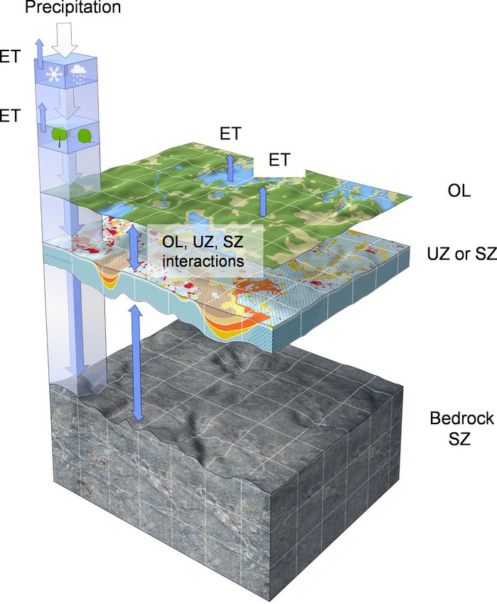
Figure 3. Schematic of a general Mike SHE model setup. Pre- bution is not significantly skewed, the SD is smaller than
cipitation falls on the ground as rain or snow. Evapotranspiration half of the average (Taagepera, 2008). In the case of the
(ET) processes include canopy interception, open surface evapora- observed δ 18 O and BC concentrations (Table 2), the SD is
tion, root uptake, and soil evaporation from the unsaturated zone much smaller than half of the average. Therefore, the arith-
(UZ). The overland flow (OL), saturated zone (SZ), and UZ interact metic mean was used to describe the central tendency of the
depending on the saturation level. The SZ is divided into 10 cal- data set. However, if the travel time distribution becomes
culation layers (CLs), while the UZ has a much finer description.
skewed, the arithmetic mean becomes highly sensitive to
Streamflow is modelled through Mike 11 and is not restricted to the
the tail of the distribution and produces considerable uncer-
Mike SHE resolution. The figure is used courtesy of SKB. Figure
illustrator: LAJ. tainty. In these cases, the median and the geometric mean
are often better as a measure of the central tendency of mean
travel time (MTT) than the average. However, to compare
the MTT of discharged water of different streams, we still
wanted the metric to account for the length of the tail. There-
Table 4. Porosity values for different soil types used in the Mike
SHE model.
fore, we used the geometric mean because the median only
states the middle value of a distribution regardless of the tail
Soil type Porosity (–) length (Taagepera, 2008; Unlu et al., 2004; Zhang and Zhang,
1996). However, we provide all metrics, including the arith-
Gravela 0.32 metic mean, geometric mean, median, and SD, in the Ap-
Sandb 0.35
pendix, Table A2.
Siltc 0.45
The MTT was compared to stream chemistry, which is a
Clayb 0.55
mix of both groundwater and surface water. In winter, all
Silt–clayd 0.50
streamflow contributions originate from groundwater. Here
Tillb 0.30
the results from the particle tracking reflect the actual travel
Peatb 0.50
Bedrockb 0.0001
time to the streams. However, in summer and especially in
Bedrock fractures/deformation zonesb 0.001
spring, some water will reach the streams via overland flow
(OL), which has not spent any time in the ground. Since the
a Average of Morris and Johnson (1967). b Joyce et al. (2010). c Average
particle tracking does not take surface flow into account, OL
value between sand and clay. d Average value between silt and clay.
was accounted for by reducing the MTT by using the OL
fraction as a scaling factor (Appendix, Table A2). The young
https://doi.org/10.5194/hess-25-2133-2021 Hydrol. Earth Syst. Sci., 25, 2133–2158, 20212142 E. Jutebring Sterte et al.: How catchment characteristics influence hydrological pathways
Figure 4. Particle model setup. (a) Steps of particle tracking. (b) Average depth to the groundwater table. The main part of the model area
has a calculated depth to the groundwater table between 0 and 3 m and varied daily. (c) Schematic illustration of particle-tracking setup.
Particles were added to groundwater recharge at the transient groundwater table. The age of these particles was zero at the time of recharge.
Thereafter, they followed the groundwater flow, increasing in age until reaching a stream or lake.
water fraction was also used as an evaluation criterion. Like metric mean of the travel time distributions provided the best
previous studies (Kirchner, 2016; von Freyberg et al., 2018; representation of MTT (Table 5, Fig. 5). However, all metrics
Lutz et al., 2018; Stockinger et al., 2019), we assumed young are stated in the Appendix, Table A2. The annual MTTgeo for
water fraction to be the sum of all water less than 3 months all sub-catchments ranged from 0.8 to 3.1 years (Table 5).
old. In our case, this includes all water reaching streams Most groundwater discharging to a stream had a travel time
as overland flow and as young groundwater (< 3 months). of less than 1 year in all sub-catchments (34 % to 54 %). The
The modelled MTT and young water fraction were also used longest stream MTTs were connected to the larger catch-
to identify the main factors determining the travel times to ments, such as C16, and the silt-dominated catchments such
stream. The catchment characteristics tested included impor- as C20. We used some sub-catchments for result represen-
tant terrain factors such as catchment size, slope, and main tation, but all results are provided in Table 5 and Appendix
soil types (Table 1). Table A2. The displayed sub-catchments were C2 (small till-
and forest-dominated catchment), C4 (small mire-dominated
catchment), C20 (small silt-dominated catchment), and C16
3 Results (the full-scale Krycklan catchment).
On an annual basis, a fraction of water reached the streams
3.1 Travel time results as overland flow. A major part of the overland flow occurred
during the snowmelt in spring, especially in sub-catchments
The particle-tracking results were used to establish travel with mires such as C4 (Fig. 6). Both the fraction of young
time distributions and MTT of water to the streams of the water reaching the streams and the MTTgeo displayed strong
14 sub-catchments in Krycklan. Since the travel time distri- seasonal trends. The longest seasonal MTTgeo , 1.2–7.7 years,
butions were significantly skewed, we assumed that the geo-
Hydrol. Earth Syst. Sci., 25, 2133–2158, 2021 https://doi.org/10.5194/hess-25-2133-2021E. Jutebring Sterte et al.: How catchment characteristics influence hydrological pathways 2143
Table 5. Annual and seasonal (winter, spring, and summer) travel times. The geometric mean of the travel time distribution (MTTgeo ) is
adjusted for the overland flow. The young water fraction (YWF) includes overland flow and groundwater younger than 3 months (%). An
extended version of the results, including arithmetic mean, median, and SD, is included in the Appendix (Table A2).
Annual Season – winter Season – spring Season – summer
MTTgeo YWF MTTgeo YWF MTTgeo YWF MTTgeo YWF
Unit Year % Year % Year % Year %
C2 0.8 16 1.2 0 0.7 26 0.7 6
C4 0.8 40 1.5 2 0.7 53 0.7 39
C5 0.8 49 2.9 1 0.5 66 0.8 38
C6 0.9 42 2.8 2 0.6 58 0.8 34
C7 1.1 28 2.2 4 0.9 37 0.9 27
C9 1.4 28 3.4 3 1.0 41 1.1 24
C13 1.4 26 3.3 3 1.0 37 1.2 23
C1 1.3 20 3.0 6 1.0 25 0.9 19
C10 1.1 33 2.5 3 0.8 47 0.9 31
C12 1.3 28 2.8 5 0.9 39 1.1 26
C14 2.4 20 5.6 2 1.6 32 1.6 21
C20 2.7 23 7.7 0 1.9 36 1.5 24
C15 1.5 28 3.8 4 0.9 41 1.1 27
C16 2.3 23 5.3 4 1.4 35 1.6 23
In spring, mire sub-catchments had the shortest MTTgeo .
However, as exemplified by the similar-sized C2 and C4 sub-
catchments, groundwater was not renewed to the same ex-
tent in mire-dominated systems due to a larger fraction of
surface runoff (Fig. 6). Mire-dominated sub-catchments (like
C4) displayed stronger seasonal variations in MTTgeo , with
shorter MTTgeo than till-dominated sub-catchments (like C2)
in spring and longer MTTgeo than C2 in winter (Table 5). In
C4, the MTTgeo decreased from 1.5 to 0.7 years from win-
ter to spring, while the corresponding change in C2 was 1.2
to 0.7 years. The seasonality of MTTgeo was even more pro-
nounced for catchments with a larger areal coverage of mires
combined with a larger areal coverage of silt. For example,
C20 had an MTTgeo that decreased from 7.7 to 1.9 years from
Figure 5. Examples of particle-tracking results. The figure shows winter to spring (Table 5).
the distribution of all particles reaching the different streams for
the entire modelling period. The solid line shows the statistics for 3.2 Testing model results on stream isotopic
C16, including the 25th percentile, the median, the geometric mean, composition and chemistry
the arithmetic mean, and the 75th percentile (Appendix A). More-
over, the figure shows three other example distributions, including In addition to investigating the annual MTTgeo , three distinct
C2 (small forest- and till-dominated catchment), C4 (small mire- seasons were evaluated regarding the stream chemistry: win-
dominated catchment), and C20 (small silt-dominated catchment).
ter, spring, and summer. The isotopic composition was avail-
able for 13 out of 14 sub-catchments (C20 excluded because
of short time series), while the BC data were available for
all sites. In winter, the modelled MTTgeo was correlated with
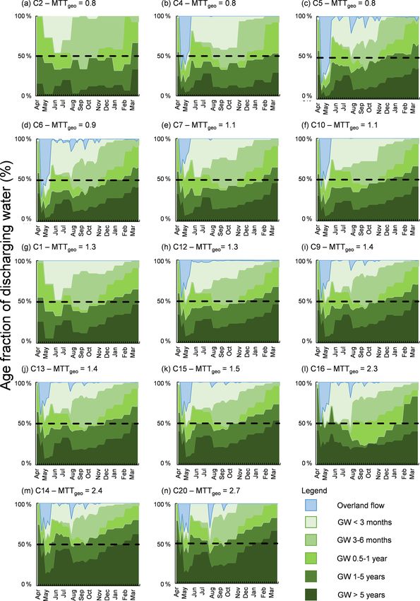
and the smallest young water fraction were found during the the isotopic composition (r = −0.80, P2144 E. Jutebring Sterte et al.: How catchment characteristics influence hydrological pathways Figure 6. Seasonal fraction of discharge to streams. The figure shows the proportion of annual stream discharge arriving as groundwater and overland flow. Four sub-catchments are exemplified, including (a) the small till- and forest-dominated C2, (b) the small mire-dominated C4, (c) the silt-dominated C20, and (d) the full-scale Krycklan catchment C16 with mixed mires and forests (extended version in Appendix Fig. A1). The figure showcases the travel time fraction of water discharging to the streams. The fractions are both shown as part of the total annual discharge as well as the water composition. The bands below the months highlight the three investigated seasons, spring, summer, and winter. the conceptual model (Fig. 2a). The same was also true for 3.3 Model results compared to catchment the summer season but with a weaker positive correlation characteristics compared to the spring (r = 0.80, P
E. Jutebring Sterte et al.: How catchment characteristics influence hydrological pathways                                    2145

were similar (Table 6). However, the positive correlation be-          Another uncertainty related to the particle-tracking model
tween mires and the young water fraction was lost in winter         in Mike SHE is related to the travel time from the point of
due to a lack of new precipitation input into the system. A         infiltration through the unsaturated soil horizons to the sat-
weak negative correlation between MTTgeo and the young              urated groundwater. Due to technical limitations, this travel
water fraction was found for the annual and spring seasonal         time cannot be accounted for in the particle-tracking calcu-
results but was lost for the summer and winter.                     lations. Particles are placed at the groundwater table propor-
                                                                    tionally to the groundwater recharge (Fig. 4). Therefore, the
                                                                    main fraction of particles introduced to the model occurs at
4     Discussion                                                    high infiltration rates when the groundwater level is close to
                                                                    the soil surface. Under these conditions, the water has, in
Particle tracking in the Mike SHE model provided valu-
                                                                    most cases, spent a relatively short time in the unsaturated
able insights into the annual and seasonal mean travel times
                                                                    zone. However, some particles are also introduced when the
(MTTgeo ) across the 14 Krycklan sub-catchments. The mod-
                                                                    groundwater level is lower, such as early snowmelt or follow-
elled MTTgeo and the young water fractions were strongly
                                                                    ing extended dry periods. Under such conditions, the model
correlated with observed stream δ 18 Owinter signatures, sea-
                                                                    uncertainty increases. In this context, the smallest potential
sonal variation in δ 18 O, and base cation (BC) concentra-
                                                                    uncertainty occurs in mires, where the groundwater table al-
tions. This model validation suggests that particle track-
                                                                    ways is close to the ground surface. The uncertainty becomes
ing is a useful complementary tool to tracer-based travel
                                                                    somewhat larger in the till areas where the unsaturated zone
time studies, at least in snow-dominated catchments, ar-
                                                                    on average is above 1 m but can extend down to 3 m be-
eas with pronounced seasonality, and streams dominated by
                                                                    low the ground during low flow. C14 and the lower part of
older groundwater (> 4 years). Overall, we found that soil
                                                                    C16 are exceptions to these relatively shallow saturated con-
type was the most important variable explaining MTTgeo
                                                                    ditions as a deep esker traverses the sub-catchments result-
and that mires are an important landscape feature regulating
                                                                    ing in a groundwater level up to 10 m below the soil surface
the young water fraction in spring (Fig. 8).
                                                                    (Fig. 1). Accounting for the travel time from infiltration to
4.1    Model assumptions and limitations of estimated               recharge could impact the results and provide, especially for
       travel times                                                 C14 and C16, longer MTT than if the groundwater level were
                                                                    at the same level throughout the whole catchment. This lim-
Comparing the results from this modelling study to previ-           itation primarily affects catchments with the longest MTTs
ous Krycklan investigations of MTT conducted in the C7              and, therefore, does not seriously question the general pat-
sub-catchment demonstrates that different model approaches          tern observed. The distance from the ground surface to the
have provided similar results. While our study suggested            groundwater table is, for most model cells, much shorter
a MTTgeo of 1.1 years and a median of 0.8 years (Ap-                than the distance to the nearest stream, so most of the transit
pendix, Table A2), Peralta-Tapia et al. (2016) calculated a         time should be related to the groundwater flow rather than
MTT of 1.8 (minimum 0.8 and maximum 3.3) years by ap-               to percolation. Although water, especially during dry condi-
plying a mathematical method for isotopic dampening to fit          tions, no doubt can spend considerable time in the unsatu-
a model to the observed stream isotopic response. In an-            rated zone, it must also be acknowledged that this water vol-
other recent study using the Spatially distributed Tracer-          ume is small compared to the groundwater inventory in the
Aided Rainfall-Runoff (STARR) model for the same stream,            saturated zone. Therefore, its impact on the average MTTs
the median age was estimated to 0.9 years (Ala-aho et al.,          should be relatively small.
2017). The close agreement between the different studies
strengthens the overall reliability of the results. However, like   4.2   Seasonality of isotopic composition
all modelling techniques, particle tracking in Mike SHE is
associated with some uncertainties and limitations.                 Following the conceptual model (Fig. 2), patterns in stream
   In contrast to the Mike SHE flow model, which esti-              isotopic signatures can be explained by seasonal changes
mates groundwater and overland flow pathways, the particle-         in travel times. The modelling results show that all sub-
tracking model is restricted to the subsurface hydrological         catchments discharged water with the longest travel times in
component. This is a limitation in the modelling approach as        winter, somewhat shorter travel times in summer, and wa-
water reaches the streams as a mix of groundwater and over-         ter with the shortest travel times in spring. When winter ar-
land flow. Therefore, to allow for actual MTTgeo estimates,         rived, the main precipitation was snow, resulting in a cessa-
we corrected the results by reducing the estimated MTTgeo           tion of the groundwater recharge. This caused an increasing
using the overland flow from the flow model as a scaling fac-       proportion of old groundwater discharging into the streams
tor (Appendix, Table A2). This uncertainty primarily affects        (Fig. 6). In agreement with our conceptual model (Fig. 2), a
the mire-dominated sub-catchments that have a large fraction        strong negative correlation between winter MTTgeo and the
of overland flow, especially during the spring.                     isotopic stream signatures during winter baseflow was ob-
                                                                    served (Fig. 7a). At an average travel time older than 4 years,

https://doi.org/10.5194/hess-25-2133-2021                                        Hydrol. Earth Syst. Sci., 25, 2133–2158, 2021
2146 E. Jutebring Sterte et al.: How catchment characteristics influence hydrological pathways Figure 7. Relationships of seasonal MTTgeo and young water fractions (YWFs) with seasonal stream isotopic composition and base cation concentration. Note that δ 18 O results are for 13 sites, while the BC record comprises all 14. The sub-plots (a) to (f) show the δ 18 O (winter) or 1δ 18 Ospring/summer and BC concentrations as a function of the MTTgeo in winter, spring, and summer, respectively. The standard error of the mean (SEM) shown as whiskers denotes variations in field observations. Figure 8. Catchment characteristics are important for travel times. The figure shows the annual averages: (a) the areal coverage of mires and the young water fraction (YWF), (b) areal coverage of silt and MTTgeo , and (c) catchment size and MTTgeo . Hydrol. Earth Syst. Sci., 25, 2133–2158, 2021 https://doi.org/10.5194/hess-25-2133-2021
E. Jutebring Sterte et al.: How catchment characteristics influence hydrological pathways                                                     2147

Table 6. Correlation matrix – young water fraction (YWF), geometric mean travel time (MTTgeo ), and catchment characteristics. The
catchment characteristics include the log catchment size (log A), the areal coverage of mires (Mire), and the areal coverage of silt (Silt). The
table includes annual, winter, spring, and summer results.

                                                             Winter season                                     Summer season
                                 Log A           Mire         Silt     MTTgeo     YWF      Log A      Mire       Silt   MTTgeo      YWF
                                 (km2 )           (%)         (%)       (year)     (%)     (km2 )      (%)       (%)     (year)      (%)
           Log A (km2 )               1        0.02        0.58 a        0.64 a   −0.08         1      0.02   0.58a       0.68a     0.20
           Mire (%)                0.02           1        −0.37         −0.34    −0.14      0.02         1    0.37      −0.50b    0.91a
           Silt (%)              0.58 a       −0.37             1        0.92 a   −0.43     0.58a    −0.37        1       0.80a    −0.20
           MTTgeo (year)         0.63b       −0.51b         0.90a             1   −0.21     0.55a   −0.55a    0.92a           1    −0.28
           YWF (%)               −0.02        0.96a        −0.39        −0.53b        1      0.11    0.95 a   −0.29      −0.52b        1
                                                     Annual                                           Spring season

         For |r|>0.5, the p value is shown according to a p0.05.

it can be expected that the groundwater has reached full mix-                      the 1δ 18 Ospring , there was still a significant correlation be-
ing. Hence, older water can no longer be accurately quanti-                        tween the average 1δ 18 Osummer and the modelled young wa-
fied using amplitude dampening of the water isotope signal                         ter fraction (Fig. 7e).
(Kirchner, 2016). These theoretical considerations strengthen
the results of a winter MTTgeo older than 4 years for some                         4.3    Controls of travel times on base cation
sub-catchments since their stream isotopic signatures were                                concentrations
close to the long-term precipitation average and, therefore,
should have reached complete mixing.                                               The annual and seasonal average BC concentrations were
   When snowmelt began in late April or early May, the                             positively correlated with the MTTgeo (Fig. 7b, d, and f).
MTTs consistently decreased in all sub-catchments. The                             Since the weathering rates were assumed to be kinetically
fraction of young groundwater in different sub-catchments                          controlled and hence related to the exposure time of wa-
was well reflected in the change in the isotope signal (Fig. 7).                   ter to minerals, spatial and temporal variability in BCs can
For snowmelt in spring, the calculated young water frac-                           be used as a relative indicator for transit time (Erlandsson
tion was used to evaluate the proportion of water reach-                           Lampa et al., 2020). However, reducing weathering to travel
ing the stream through rapid pathways, including overland                          times may be an oversimplification as the rate is also affected
flow. It is well established that the difference in stream iso-                    by differences in mineralogy, particle size distributions and
topic signature between winter baseflow and spring peak                            the chemical conditions in the groundwater. However, previ-
flow at snowmelt (1δ 18 Ospring ) is mechanistically linked to                     ous research in the Krycklan catchment has suggested that
the amount of new water reaching the stream (Tetzlaff et al.,                      the chemical composition of the local mineral soils is sur-
2009). In agreement with this, we found a strong statistical                       prisingly homogeneous, even when comparing till and sorted
relationship between 1δ 18 Ospring and the calculated young                        sediments (Klaminder et al., 2011; Peralta-Tapia et al., 2015;
water fraction (Fig. 7c). These results are well in line with                      Erlandsson et al., 2016; Lidman et al., 2016). Therefore, we
previous work in Krycklan using end-member mixing of new                           did not expect mineralogical differences between soil types
and old water in the same streams (Laudon et al., 2004, 2007,                      to impact the release of cations significantly. However, one
2011).                                                                             exception is peat deposits, which strongly affect the cation
   Similarly to the conditions in spring, the conceptual model                     concentrations on the landscape scale. The effect of the peat
predicted that the difference in stream isotopic signature                         was accounted for by adjusting the concentrations following
between winter baseflow and summer flow, 1δ 18 Osummer ,                           Lidman et al. (2014). Differences in particle size distribution
should be correlated with the young water fraction in summer                       may be important because coarser soils will have less sur-
but with the opposite sign, due to isotopically heavier sum-                       face area per volume unit, allowing for less weathering. How-
mer rains (Fig. 2). A larger inter-annual variation in precip-                     ever, such soils can also be expected to have higher hydraulic
itation and high ET likely caused the relationship to be less                      conductivities, leading to higher flow velocities and, conse-
evident compared to the spring results as the snowmelt con-                        quently, less time available for weathering. Therefore, dif-
ditions are more consistent from year to year. The ground-                         ferences in area–volume ratios between different soil types
water signal reaching the streams during the summer sea-                           would not counteract the effect of travel times on the weath-
son may also be affected by a lingering signal from the                            ering but rather enhance it.
snowmelt. However, although less evident than compared to                             Despite arguments that can be made against the use of
                                                                                   BCs as tracers, they still offer a complementary possibility

https://doi.org/10.5194/hess-25-2133-2021                                                       Hydrol. Earth Syst. Sci., 25, 2133–2158, 2021
You can also read