Insight into PM2.5 sources by applying positive matrix factorization (PMF) at urban and rural sites of Beijing
←
→
Page content transcription
If your browser does not render page correctly, please read the page content below
Atmos. Chem. Phys., 21, 14703–14724, 2021
https://doi.org/10.5194/acp-21-14703-2021
© Author(s) 2021. This work is distributed under
the Creative Commons Attribution 4.0 License.
Insight into PM2.5 sources by applying positive matrix factorization
(PMF) at urban and rural sites of Beijing
Deepchandra Srivastava1 , Jingsha Xu1 , Tuan V. Vu1,a , Di Liu1,2 , Linjie Li2 , Pingqing Fu3 , Siqi Hou1 ,
Natalia Moreno Palmerola4 , Zongbo Shi1 , and Roy M. Harrison1,b
1 School of Geography Earth and Environmental Science, University of Birmingham, Birmingham, B15 2TT, UK
2 Institute of Atmospheric Physics, Chinese Academy of Science, Beijing, 100029, China
3 Institute of Surface-Earth System Science, Tianjin University, Tianjin, 300072, China
4 Laboratori de Raigs-X, Institute of Environmental Assessment and Water Research (IDÆA), Consejo Superior de
Investigaciones Científicas (CSIC), C/Jordi Girona, 18-26, 08034 Barcelona, Spain
a now at: School of Public Health, Imperial College London, London, UK
b also at: Department of Environmental Sciences/Centre of Excellence in Environmental Studies, King Abdulaziz University,
P.O. Box 80203, Jeddah, 21589, Saudi Arabia
Correspondence: Roy M. Harrison (r.m.harrison@bham.ac.uk) and Zongbo Shi (z.shi@bham.ac.uk)
Received: 30 September 2020 – Discussion started: 7 April 2021
Revised: 30 July 2021 – Accepted: 13 August 2021 – Published: 5 October 2021
Abstract. This study presents the source apportionment of balance – CMB) and PMF performed on other measurements
PM2.5 performed by positive matrix factorization (PMF) on (i.e. online and offline aerosol mass spectrometry, AMS) and
data presented here which were collected at urban (Institute showed good agreement for some but not all sources. The
of Atmospheric Physics – IAP) and rural (Pinggu – PG) sites biomass burning factor in PMF may contain aged aerosols
in Beijing as part of the Atmospheric Pollution and Human as a good correlation was observed between biomass burn-
Health in a Chinese megacity (APHH-Beijing) field cam- ing and oxygenated fractions (r 2 = 0.6–0.7) from AMS. The
paigns. The campaigns were carried out from 9 November PMF failed to resolve some sources identified by the CMB
to 11 December 2016 and from 22 May to 24 June 2017. The and AMS and appears to overestimate the dust sources. A
PMF analysis included both organic and inorganic species, comparison with earlier PMF source apportionment studies
and a seven-factor output provided the most reasonable so- from the Beijing area highlights the very divergent findings
lution for the PM2.5 source apportionment. These factors from application of this method.
are interpreted as traffic emissions, biomass burning, road
dust, soil dust, coal combustion, oil combustion, and sec-
ondary inorganics. Major contributors to PM2.5 mass were
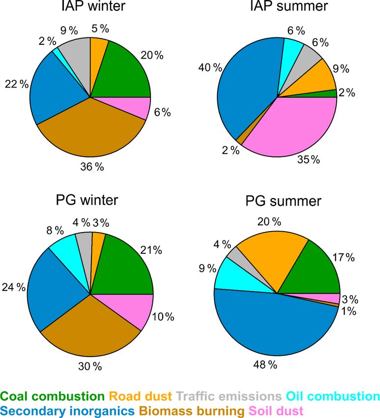
secondary inorganics (IAP: 22 %; PG: 24 %), biomass burn- 1 Introduction
ing (IAP: 36 %; PG: 30 %), and coal combustion (IAP: 20 %;
PG: 21 %) sources during the winter period at both sites. Sec- Atmospheric particulate matter (PM) is composed of various
ondary inorganics (48 %), road dust (20 %), and coal com- chemical components and can affect air quality (and conse-
bustion (17 %) showed the highest contribution during sum- quently human health), visibility, and ecosystems (Boucher
mer at PG, while PM2.5 particles were mainly composed of et al., 2013; Heal et al., 2012). Through absorption and scat-
soil dust (35 %) and secondary inorganics (40 %) at IAP. De- tering of solar radiation and by affecting clouds, PM also
spite this, factors that were resolved based on metal signa- has a major impact on the climate and thus the hydrologi-
tures were not fully resolved and indicate a mixing of two or cal cycle. PM with an aerodynamic diameter less than 2.5 µm
more sources. PMF results were also compared with sources (PM2.5 ) is given special attention due to its adverse effects on
resolved from another receptor model (i.e. chemical mass human health as it can penetrate deep into human lungs when
inhaled. Several recent studies have indicated that many ad-
Published by Copernicus Publications on behalf of the European Geosciences Union.
14704                                                              D. Srivastava et al.: Insight into PM2.5 sources using PMF

verse health outcomes, such as respiratory and cardiovascu-         as the input data matrix to explore the co-variances between
lar morbidity and mortality, are related to long-term expo-         species and their associated sources, but to the best of our
sure to PM (Lu et al., 2021; Wang et al., 2016; Xing et al.,        knowledge, the use of organic markers in PMF has not been
2016; Xie et al., 2019). In addition, over a million prema-         explored extensively in Beijing. The use of organic molecu-
ture deaths per year are reported in China due to poor air          lar markers in PMF has enhanced our understanding of the
quality (GBD MAPS Working Group, 2016). Beijing, the                PM fraction as they can be source specific (Shrivastava et al.,
capital city of China, is a megacity with approximately 21          2007; Jaeckels et al., 2007; Zhang et al., 2009; Wang et al.,
million inhabitants that are regularly exposed to severe haze       2012; Srimuruganandam and Shiva Nagendra, 2012; Schem-
events. For example, 77 pollution episodes (defined as 2 or         bari et al., 2014; Laing et al., 2015; Waked et al., 2014; Sri-
more consecutive days where the average PM2.5 concentra-            vastava et al., 2018) and could potentially offer a clearer link
tion exceeds 75 µg m−3 ) were observed between April 2013           between factors and sources.
and March 2015 (Batterman et al., 2016). PM2.5 concentra-              This study presents the results obtained from the PMF
tions have reached 1000 µg m−3 in some heavily polluted ar-         model applied to a filter-based dataset collected in the Bei-
eas of Beijing (Ji et al., 2014). In addition, a study compared     jing metropolitan area at two sites, urban and rural. The study
the number of cases of acute cardiovascular, cerebrovascular,       provides source apportionment results from both urban and
and respiratory diseases in the Beijing Emergency Center and        rural locations in Beijing, including their temporal and spa-
haze data from Beijing Observatory between 2006 and 2013.           tial variations. In addition, the study also presents a short
Their results showed a rising trend, highlighting that the aver-    summary of previously published filter-based studies con-
age number of cases per day for all three diseases was higher       ducted in the Beijing metropolitan area and their major out-
on hazy days than on non-hazy days (Zhang et al., 2015).            comes. A comparison of the present PMF results was also
Therefore, major control measures were implemented to re-           made with other source apportionment approaches or appli-
duce PM2.5 pollution in Beijing (Vu et al., 2019). Recently,        cations of PMF to other datasets, with an aim of discussing
one-third of Chinese cities in 2020 were kept under lockdown        the existing PM sources in the Beijing metropolitan area, in-
to prevent the transmission of the COVID-19 virus, which            cluding focussing on the strengths and weaknesses of the
strictly curtailed personal mobility and economic activities.       source apportionment approach employed.
The lockdown led to an improvement in air quality and man-
aged to bring down the levels of PM2.5 . Despite these im-
provements, PM2.5 concentrations during the lockdown peri-          2     Methodology
ods remained higher than the World Health Organization rec-
ommendations, suggesting much more effort is needed (He             Details about the sampling site, measurements, sample col-
et al., 2020; Le et al., 2020; Shi et al., 2021). A quantitative    lection, and analytical procedures are reported elsewhere
source apportionment provides key information to support            (Shi et al., 2019; Xu et al., 2021; Wu et al., 2020), and hence
such efforts.                                                       only the essential information is presented in this section.
   Receptor models are widely used for source apportion-
ment of PM2.5 . These methods include positive matrix fac-          2.1    Sampling site and sample collection
torization (PMF) (Paatero, 1997; Paatero and Tapper, 1994),
principal component analysis (PCA) (Lee and Hieu, 2011),            The PM2.5 sampling was conducted simultaneously at the ur-
chemical mass balance (CMB) (Watson et al., 1990), and              ban and rural sites from 9 November to 12 December 2016
UNMIX (Herrera Murillo et al., 2012). Among these meth-             and from 22 May to 24 June 2017 as part of the Atmospheric
ods, PMF is a widely used multivariate method that can re-          Pollution and Human Health in a Chinese megacity (APHH-
solve the dominant positive factors without prior knowledge         Beijing) field campaigns (Shi et al., 2019) (Fig. S1). The ur-
of sources. Previous PMF studies, based on high-resolution          ban sampling site (116.39◦ E, 39.98◦ N) – the Institute of At-
aerosol mass spectrometer data, have provided valuable in-          mospheric Physics (IAP) of the Chinese Academy of Sci-
formation on the sources of PM in urban Beijing and its sur-        ences in Beijing – represents a typical condition of central
rounding areas (Huang et al., 2010; Sun et al., 2010, 2013;         Beijing: there are various roads nearby, including a highway
Zhang et al., 2013, 2014, 2015, 2016, 2017; Hu et al., 2016;        road approximately 200 m away. The rural Pinggu site (PG)
Qiu et al., 2019). However, the factors that influence haze for-    (40.17◦ N, 117.05◦ E) is located in Xibaidian. This site is ap-
mation and related sources remain unclear due to its inherent       proximately 60 km to the north-east of the Beijing city centre
complexity (Tie et al., 2017; Sun et al., 2014). Filter-based       and about 4 km north-west of the Pinggu town centre. The
PMF studies provide a valuable tool for identifying sources         site is surrounded by trees and farmland. In addition, resi-
of airborne particles, by utilizing size-resolved chemical in-      dents mainly use coal and biomass for heating and cooking
formation (Li et al., 2019; Ma et al., 2017a; Tian et al., 2016;    in individual homes.
Yu et al., 2013; Song et al., 2007, 2006). These source appor-         Twenty-four-hour PM2.5 samples were collected every
tionment studies have predominantly used OC (organic car-           day on pre-baked quartz filters (Pallflex, 20 × 25 cm) and
bon), EC (elemental carbon), water-soluble ions, and metals         47 mm polytetrafluoroethylene (PTFE) filters (flow rate of

Atmos. Chem. Phys., 21, 14703–14724, 2021                                           https://doi.org/10.5194/acp-21-14703-2021
D. Srivastava et al.: Insight into PM2.5 sources using PMF                                                                 14705

15.0 L min−1 ) using high-volume (Tisch, USA, flow rate of         included quantification of similar species (12 n-alkanes C24 -
1.1 m3 min−1 ) and medium-volume (Thermo Scientific Par-           C35 , 9 hopanes, 22 PAHs, 3 anhydrous sugars (levoglucosan,
tisol 2025i) air samplers. Field blanks were also collected        mannosan, galactosan), 4 fatty acids (palmitic acid, stearic
during the sampling campaign at both sites. The quartz fil-        acid, linoleic acid, oleic acid), and cholesterol) with few ad-
ters were then analysed for organic tracers, OC / EC, and          ditional ones. Recoveries for the identified organic tracers
ion species. PTFE filters were used for the determination of       ranged from 70 % to 100 % and from 80 % to 110 % at IAP
PM2.5 mass and metals. Details on preparation and conserva-        and PG, respectively. Field blanks were also analysed as part
tion of these filter samples have already been reported else-      of quality control and demonstrated very low contamination
where (Wu et al., 2020; Xu et al., 2021).                          (< 5 %).
   Real-time composition of non-refractory PM1 particles              In addition, one or two punches of PM2.5 filter sample
(NR-PM1 ) was measured using an Aerodyne aerosol mass              were also analysed offline using AMS to investigate the
spectrometer (AMS) at a time resolution of 2.5 min. The op-        water-soluble OA (WSOA) mass spectra following the pro-
erational details on the AMS measurements have been given          cedure explained previously (Qiu et al., 2019).
elsewhere (Xu et al., 2019). In addition, the measurements
of gaseous species such as O3 , CO, NO, NO2 , and SO2 were         2.3     Positive matrix factorization
performed using gas analysers. The meteorological parame-
ters, including temperature (T), relative humidity (RH), wind      Detailed information on the receptor modelling methods
speed (WS), and wind direction (WD), were also measured            used within this study can be found elsewhere (Paatero and
at both sites.                                                     Tapper, 1994; Hopke, 2016). PMF is a multivariate fac-
                                                                   tor analysis tool and based on a weighted least-squares fit,
2.2   Analytical procedure                                         where the weights are derived from the analytical uncer-
                                                                   tainty. The best model solution was obtained by minimiz-
In total, 62 and 72 chemical species were quantified in each       ing residuals obtained between modelled and observed input
PM2.5 sample from IAP and PG, respectively. This included          species concentrations. Estimation of analytical uncertain-
EC / OC, 36 organic tracers, 7 major inorganic ions (Na+ ,         ties for the filter-based measurements was calculated using
K+ , Ca2+ , NH+       −     −         2−                           Eq. (1) (Polissar et al., 1998).
                4 , Cl , NO3 , and SO4 ), and 17 metallic el-
ements (V, Cr, Co, Mn, Ni, Cu, Zn, As, Br, Sr, Ag, Cd, Sn,                ( 5
                                                                              6 LDj                         if Xij < LDj ,
Sb, Ba, Hg, and Pb) at IAP. Similarly, the identified species at   σij = q                                                 (1)
PG included EC / OC, 51 organic tracers, 7 major inorganic                      (0.5 × LDj )2 + (EFj Xij )2 if Xij ≥ LDj ,
ions, and 12 metallic elements (V, Cr, Co, Mn, Ni, Cu, Zn,         where LDj is the detection limit for compound j and EFj is
As, Sr, Sb, Ba, and Pb). EC and OC measurements were per-          the error fraction for compound j . The detection limits of all
formed using a Sunset lab analyser (model RT-4) and a DRI          compounds used in the PMF model are given in Table S1
multi-wavelength thermal–optical carbon (model 2015) anal-         (Supplement). The U.S. Environmental Protection Agency
yser based on the EUSAAR2 (European Supersites for At-             (US-EPA) PMF 5.0 software was used in this work to per-
mospheric Aerosol Research) transmittance protocol at both         form the source apportionment.
sites, IAP and PG, respectively, following the procedure ex-
plained by Paraskevopoulou et al. (2014). Major inorganic          2.3.1    Selection of the input data
ions and metallic elements were analysed using an ion chro-
matograph (Dionex, Sunnyvale, CA, USA) and inductively             The selection of species used as input data for the PMF anal-
coupled plasma-mass spectrometer (ICP-MS) at both sites,           ysis is important and can significantly influence the model
respectively. Major crustal elements including Al, Si, Ca, Ti,     results (Lim et al., 2010). The following set of criteria was
and Fe were determined by an X-ray fluorescence spectrom-          used for the selection of the input species: signal-to-noise
eter (XRF).                                                        ratio (S / N) (Paatero and Hopke, 2003), major PM chemical
   Organic tracers at IAP included 11 n-alkanes C24 -C34 ,         species, compounds with maximum data points above the
2 hopanes, 17 polycyclic aromatic hydrocarbons (PAHs),             detection limit, and those being considered specific markers
3 anhydrous sugars (levoglucosan, mannosan, galactosan),           of a given source (e.g. levoglucosan, picene) (Oros and
2 fatty acids (palmitic acid, stearic acid), and cholesterol.      Simoneit, 2000; Simoneit, 1999) were selected. These
These organic tracers were analysed by gas chromatography–         steps were taken to limit the input data matrix according
mass spectrometry (GC–MS, Agilent 7890A GC plus 5975C              to the total number of samples (n = 133); some species
mass-selective detector) coupled with a DB-5MS col-                were also not included if they belonged to a single source
umn (30 m × 0.25 mm × 0.25 µm) following the protocol ex-          and correlated with another marker of this source. A total
plained in Xu et al. (2020). At PG, organic tracers were anal-     of 31 species were used in the model (PM2.5 , OC, EC,
                                                                                                       2−
ysed based on the method reported by Wu et al. (2020) us-          K+ , Na+ , Ca2+ , NH+        −             −
                                                                                          4 , NO3 , SO4 , Cl , Ti, V, Mn, Ni,
ing GC/MS (Agilent GC-6890N plus MSD-5973N) coupled                Zn, Pb, Cu, Fe, Al, C26, C29, C31, 17α(H)-22,29,30-
with an HP-5MS column (30 m × 0.25 mm × 0.25 µm). This             trisnorhopane,17β(H),21α(H)-30-norhopane,chrysene,

https://doi.org/10.5194/acp-21-14703-2021                                         Atmos. Chem. Phys., 21, 14703–14724, 2021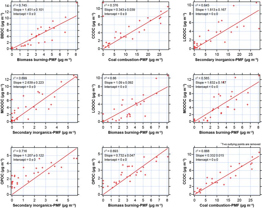
14706                                                                D. Srivastava et al.: Insight into PM2.5 sources using PMF

benzo(b)fluoranthene, benzo(a)pyrene, picene, coronene,               2.5    Other receptor modelling approaches
levoglucosan, and stearic acid). The concentration of PM2.5
was included as a total variable in the model (with large             Sources were also resolved at both sites separately using an-
uncertainties) to directly determine the source contributions         other receptor model known as CMB as well as PMF per-
to the daily mass concentrations.                                     formed on high-resolution AMS data collected at IAP. De-
                                                                      tails on sources resolved using these approaches are reported
2.3.2    Selection of the final solution                              elsewhere (Wu et al., 2020; Xu et al., 2021; Sun et al., 2020).
                                                                          Briefly, CMB is based on a linear least-squares approach
As recommended, a detailed evaluation of factor profiles,             and accounts for uncertainties in both source profiles and
temporal trends, fractional contribution of major species to          ambient measurements to apportion the sources of OC. The
each factor, and correlations with external tracers were inves-       US EPA CMB8.2 software was used for this purpose at both
tigated carefully to select the appropriate number of factors.        sites. The source profiles applied in the model were taken
   A few constraints were also applied to the base run to ob-         from local studies to better represent the sources, including
tain clearer chemical factor profiles in the final solution. The      profiles of straw burning (Zhang et al., 2007), wood burning
general framework for applying constraints to PMF solutions           (Wang et al., 2009), gasoline and diesel vehicles (Cai et al.,
has already been discussed elsewhere (Amato et al., 2009;             2017), industrial and residential coal combustion (Zhang et
Amato and Hopke, 2012). The changes in the Q values were              al., 2008), and cooking (Zhao et al., 2015). Only the source
considered here as a diagnostic parameter to provide insight          profile for vegetative detritus (Rogge et al., 1993; Wang et
into the rotation of factors. All model runs were carefully           al., 2009) was not available from local studies. The selected
monitored by examining the Q values obtained in the robust            fitting species included EC, anhydrous sugar (levoglucosan),
mode. To limit change in the Q value, only “soft-pulling”             fatty acids, PAHs, hopanes, and alkanes.
constraints were applied. The change in Q robust was < 1 %,
which is acceptable as per PMF guidelines (< 5 %) (Norris
et al., 2014). Finally, three criteria were used to select the op-
                                                                      3     Results and discussion
timal solution, including correlation coefficient (r) between
the measured and modelled species, bootstrap, and t test              3.1    Overview of PM sources in Beijing based on the
(two-tailed paired t test) performed on the base and con-                    current source apportionment study
straint runs, as explained previously (Srivastava et al., 2018).
                                                                      A seven-factor output provided the most reasonable solution
2.4     Back trajectories and geographical origins
                                                                      for the PM2.5 source apportionment performed on the com-
The geographical origin of selected identified sources and            bined dataset from IAP and PG (Figs. 1 and 2).
pollutants was investigated using concentration-weighted                 Based on the factor profiles, we identified traffic emis-
trajectory (CWT), non-parametric wind regression (NWR),               sions, biomass burning, road dust, soil dust, coal combus-
and cluster analysis methods. NWR combines ambient con-               tion, oil combustion, and secondary inorganics. For the same
centrations with co-located measurements of wind direction            dataset, solutions with six sources were less explanatory
and speed and highlights wind sectors that are associated             and some factors were mixed. Conversely, an increase in
with high measured concentrations (Henry et al., 2009). The           the number of factors led to the split of meaningful fac-
general principle is to smooth the data over a fine grid, so          tor profiles. In the final solution, the comparison of the re-
that a weighted concentration could be estimated by any               constructed PM2.5 contributions from all sources with mea-
wind direction (φ)/wind speed (v) couple, where the weigh-            sured PM2.5 concentrations for different seasons at both sites
ing coefficients are determined through Gaussian-like func-           showed good mass closure (r 2 = 0.61–0.91, slope = 0.99–
tions. CWT and cluster analysis assess the potential trans-           1.12, p < 0.05, ODR – orthogonal distance regression). A
port of pollution over a large geographical scale (Polissar et        low r 2 (0.61) value was observed for the summer period
al., 2001). These approaches combine atmospheric concen-              at IAP (Fig. S2). This may be due to the inability of PMF
trations measured at the receptor site with back trajectories         to model low concentrations observed for sources such as
and residence time information and help to geographically             biomass burning and coal combustion during the summer. In
evaluate air parcels responsible for high concentrations. For         addition, most of the species showed good agreement with
this purpose, hourly 24 h back trajectories arriving at 200 m         measured concentrations (Table S2). Bootstrapping on the fi-
above sea level were calculated from the PC-based version             nal solution showed stable results with more than 95 out of
of HYSPLIT v4.1 (Stein et al., 2015; Draxler, 1999). NWR,             100 bootstrap-mapped factors (Table S3). Finally, no signifi-
CWT calculations, and cluster analysis were performed us-             cant difference (p > 0.05) was observed in the factor chemi-
ing the ZeFir Igor package (Petit et al., 2017).                      cal profiles between the base and constrained runs (Table S4).
                                                                         Overall, secondary inorganics, biomass burning, and coal
                                                                      combustion sources were the main contributors to the total
                                                                      PM2.5 mass during winter (Fig. 3). These sources accounted

Atmos. Chem. Phys., 21, 14703–14724, 2021                                              https://doi.org/10.5194/acp-21-14703-2021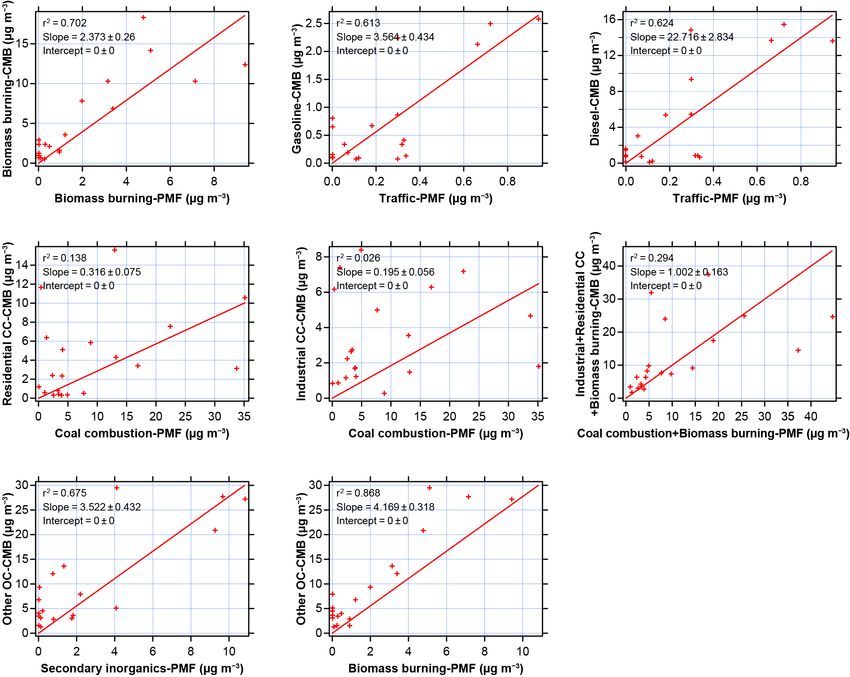
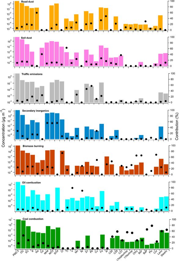
D. Srivastava et al.: Insight into PM2.5 sources using PMF                                                                       14707

Figure 1. Chemical profiles for the identified factors at IAP and PG. The bars show the composition profile (left axis) and the dots the
Explained Variation (right axis).

https://doi.org/10.5194/acp-21-14703-2021                                            Atmos. Chem. Phys., 21, 14703–14724, 2021
14708                                                                  D. Srivastava et al.: Insight into PM2.5 sources using PMF

Figure 2. Temporal variation of the identified factors at IAP and PG. Solid and broken lines represent IAP and PG, respectively.

for 22 %, 36 %, 20 % and 24 %, 30 %, 21 % of PM2.5 mass at              3.1.1    Coal combustion
IAP and PG, respectively. Secondary inorganics, road dust,
and coal combustion showed the highest contribution dur-                Coal combustion was identified based on it accounting for
ing summer at PG, while PM2.5 particles were mainly com-                a high proportion of PAHs (27 %–78 %), especially picene
posed of soil dust and secondary inorganics at IAP. Identified          (78 %) as a specific marker of coal combustion (Oros and
aerosol sources, factor profiles, and temporal evolutions are           Simoneit, 2000), together with significant amounts of OC
discussed below. Note that PMF was carried out on the com-              (45 %) and EC (29 %) (Fig. 1). This factor also made a sub-
bined datasets and thus only provides a single set of factor            stantial contribution to n-alkanes (28 %–58 %), stearic acid
profiles for both sites. Similar to previous studies (Li et al.,        (64 %), and hopanes (53 %–56 %), as these compounds are
2019; Ma et al., 2017a; Tian et al., 2016; Yu et al., 2013; Liu         also abundant in coal smoke (Bi et al., 2008; Zhang et al.,
et al., 2019; Zhang et al., 2013), neither secondary organic            2008; Oros and Simoneit, 2000; Guo et al., 2015).
aerosol nor cooking emissions were identified and, given the               The coal combustion factor accounted for 20 % of the
good mass closure, they must be present within other source             PM mass (16.0 µg m−3 ) at the urban site IAP during win-
categories.                                                             ter and followed typical seasonal variations. The contribu-
                                                                        tions of this source to PM2.5 mass were broadly similar
                                                                        (21 % vs. 17 %, Fig. 3) at PG during both seasons, while the
                                                                        average concentrations were higher in winter than summer
                                                                        (19.4 µg m−3 > 4.6 µg m−3 ). Due to a lack of infrastructure at

Atmos. Chem. Phys., 21, 14703–14724, 2021                                                 https://doi.org/10.5194/acp-21-14703-2021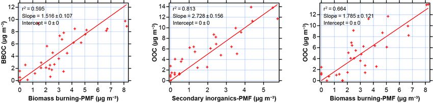
D. Srivastava et al.: Insight into PM2.5 sources using PMF                                                                   14709

                                                                    ence of local activities during the winter period at both sites.
                                                                    Higher levels of this source were observed at the rural site PG
                                                                    (19.4 µg m−3 vs. 16.0 µg m−3 at the urban site). However, a
                                                                    south-westerly flow was dominant during summer and could
                                                                    be related to transport of air masses from Hebei province,
                                                                    where a large number of industries operate.

                                                                    3.1.2   Oil combustion

                                                                    The oil combustion factor profile included high contributions
                                                                    to V (79 %) and Ni (70 %) (see Fig. 1). V and Ni are widely
                                                                    used markers for oil combustion in residential, commercial,
                                                                    and industrial applications (Viana et al., 2008; Mazzei et al.,
                                                                    2008; Pant et al., 2015; Huang et al., 2021). The V / Ni ratio
                                                                    obtained in this study was 0.9, close to the previously ob-
                                                                    tained ratio for residual oil used in power plants (Swietlicki
                                                                    and Krejci, 1996). Results suggest this source might be at-
                                                                    tributed to residual oil combustion linked to industrial ac-
                                                                    tivities as a large number of highly polluting industries are
                                                                    still located in the Beijing neighbourhood (Li et al., 2019).
                                                                    CWT and NWR analysis suggested the influence of regional
Figure 3. Contribution of different sources to PM2.5 mass at IAP    transport at both sites, highlighting the dominance of south-
and PG.                                                             westerly and south-easterly flows during the winter and sum-
                                                                    mer at both sites (Fig. S4).
                                                                       The source did not show any seasonal pattern (Fig. 2)
the rural site PG, the residents still used coal for cooking and    and accounted for 2 % (1.4 µg m−3 ) and 6 % (1.6 µg m−3 )
heating purposes at the time of sampling (Shi et al., 2019).        at IAP and 8 % (7.1 µg m−3 ) and 9 % (2.1 µg m−3 ) at PG
There is a reduction in coal usage for heating due to elevated      of the PM2.5 mass during winter and summer, respectively
temperatures in the summertime, leading to low levels of this       (Fig. 3). The contribution of this source to the PM mass was
factor at IAP. However, the similar contribution at the rural       within a similar range to the previous study conducted at the
site could be linked to consistent cooking activities through-      nearby urban site (contribution 4.7 %) (Li et al., 2019), which
out the year (Fig. 2) (Shi et al., 2019; Tao et al., 2018). These   also found a high proportion of V attributed to the identified
results were in good agreement with previous observations           source.
reported at the same urban site (18 %) (Ma et al., 2017a; Tian
                                                                    3.1.3   Biomass burning
et al., 2016). In addition, similar contributions were also ob-
served at other urban locations around Beijing (Wang et al.,        The biomass burning factor was characterized by high contri-
2008; Liu et al., 2019).                                            butions to Cl− (74 %), K+ (27 %), and levoglucosan (25 %)
   This factor also included significant contributions from         (Fig. 1). This factor also made significant contributions to
levoglucosan (60 %). Levoglucosan, a major pyrolysis prod-          PAHs (Chry: 66 %, B[b]F: 66 %, and Cor: 68 %) and fol-
uct of cellulose, has been proposed as a molecular marker           lowed a clear seasonal variation with a higher contribution
of biomass burning aerosols (Simoneit, 1999). A study con-          in winter (Fig. 2). It accounted for 36 % (29.0 µg m−3 ) and
ducted in China suggested that residential coal combustion          30 % (27.3 µg m−3 ) of the PM2.5 mass during the winter-
can also contribute significantly to levoglucosan emissions,        time at IAP and PG, respectively (Fig. 3), while the contri-
based on both source testing and ambient measurements (Yan          bution during the summertime was extremely low. This was
et al., 2018). Therefore, it is expected that the contribution of   expected due to elevated temperature during the summer pe-
levoglucosan is probably linked to residential coal use for         riod and reduction in biomass burning activities. In addition,
cooking in this case. It is possible that the high contribution     NO−                    +
                                                                        3 (24 %) and NH4 (24 %) also contributed significantly
of levoglucosan could also be linked to model bias as the           to the biomass burning factor. Biomass burning is an impor-
PMF model only provides average factor profiles for both            tant natural source of NH3 (Zhou et al., 2020) which rapidly
sites irrespective of their nature (rural vs. urban) and differ-    reacts with HNO3 to form NH4 NO3 aerosols. The presence
ent sampling periods (summer vs. winter).                           of NH4 NO3 aerosols in biomass burning plumes has also
   High concentrations of this source and levoglucosan were         been reported previously (Paulot et al., 2017; Zhao et al.,
observed at low wind speeds (Fig. S3), indicating the sig-          2020).
nificant role of local activities. This was further supported
by NWR and CWT analyses, which also showed the influ-

https://doi.org/10.5194/acp-21-14703-2021                                         Atmos. Chem. Phys., 21, 14703–14724, 2021
14710 D. Srivastava et al.: Insight into PM2.5 sources using PMF
It was unexpected to observe a low contribution of lev- it should be noted that the sampling site and dates of sam-
oglucosan, a known biomass burning marker, to this fac- pling differed. We also noticed the source profile reported
tor. However, model bias and the contribution of other rel- by Liu et al. (2019) contained the majority of all measured
evant sources to levoglucosan could have caused such obser- secondary inorganic species (> 70 %) as well as 20 % of OC,
vations, as discussed above. K+ is also produced from the while the factor identified in the present study only accounted
combustion of wood lignin and has been used extensively for ∼ 55 % of secondary inorganic species and 11 % of OC
as an inorganic tracer to apportion biomass burning contri- with the remaining fractions identified in other factors. Thus,
butions to ambient aerosol (Zhang et al., 2010; Lee et al., although the identification of the factor was “secondary” in
2008a). However, the contribution of K+ to this factor was both studies, they do not represent exactly the same source.
relatively low, possibly because K+ also has other sources, The modelled difference in the contribution of this factor to
such as soil dust (Duvall et al., 2008). Cl− can be emit- PM mass may also be related to the uncertainties of the input
ted from both coal combustion and biomass burning, espe- species: a filter-based dataset was used in the present study,
cially during the cold period in Beijing (Sun et al., 2006). while Liu et al. (2019) used online measurements.
It is also important to note that high Cl− levels observed in The highest contribution to the PM mass was observed
this factor could be associated with coal combustion (Wang during the summertime, with average concentrations of
et al., 2008). If we consider this, high Cl− levels related to 11.1 µg m−3 (40 %) and 13.2 µg m−3 (48 %) at IAP and PG,
the coal combustion factor should have also shown a sig- respectively (Fig. 3).
nificant contribution to PM mass during the summertime at
the rural site (PG) as residents near the rural site mostly use 3.1.5 Traffic emissions
coal and biomass for cooking activities as discussed above,
but they do not. Results suggest this factor can be attributed The traffic emissions factor showed relatively high contribu-
mainly to biomass burning aerosols in the Beijing metropoli- tions to metallic elements, such as Zn (47 %), Pb (57 %), Mn
tan area, but some influence of coal combustion signals can- (27 %), and Fe (22 %) (Fig. 1). Zn is a major additive to lu-
not be ignored. Back-trajectory analysis also confirmed the bricant oil. Zn and Fe can also originate from tyre abrasion,
local origin of this source during the wintertime at both sites brake linings, lubricants, and corrosion of vehicular parts and
(Fig. S5). tailpipe emission (Pant and Harrison, 2012, 2013; Grigoratos
The source contribution reported in the present study was and Martini, 2015; Piscitello et al., 2021). As the use of Pb
higher than that found in earlier studies in Beijing (11 %– additives in gasoline has been banned since 1997 in Bei-
20 %) (Li et al., 2019; Ma et al., 2017a; Tian et al., 2016; Yu jing, the observed Pb emissions may be associated with wear
et al., 2013; Song et al., 2007, 2006; Liu et al., 2019), sug- (tyre/brake) rather than fuel combustion (Smichowski et al.,
gesting some inclusion of coal burning. As both these sources 2007). These results suggest the contribution of both exhaust
follow a similar typical seasonal variation, i.e. high concen- and non-exhaust traffic emissions to this factor. Further quan-
tration during the cold period, it makes their separation diffi- tification of different types of non-exhaust emissions are hard
cult due to correlation. to predict as these metal concentrations varies according to
several parameters, such as traffic volume and patterns, ve-
3.1.4 Secondary inorganics hicle fleet characteristics, and the climate and geology of the
region (Duong and Lee, 2011).
Secondary inorganics were typically characterized by high Traffic sources accounted for 9 % and 6 % of PM2.5 mass
2−
contributions to NO− +
3 , SO4 , and NH4 (55 %, 56 %, and during the wintertime and summertime at IAP (Fig. 3),
56 % of the total species mass, respectively) (Fig. 1). This corresponding to average concentrations of 7.4 µg m−3 and
factor showed a temporal variation, with remarkably high 1.8 µg m−3 , respectively. In addition, a low contribution
concentrations observed during the period of high RH and (4 %) was observed at PG during both seasons, as PG ex-
low ozone concentration in the winter (Fig. S6). The het- periences a low traffic volume. The contribution of the traffic
erogeneous reactions on pre-existing particles in the pol- source to the PM2.5 mass was found to be low compared to
luted environment under high-RH and low-ozone conditions other studies conducted in the Beijing area (14 %–20 %) (Li
have been shown to play a key role in the formation of sec- et al., 2019; Tian et al., 2016; Yu et al., 2013; Liu et al., 2019),
ondary aerosols compared to gas-phase photochemical pro- with the exception of a study by Ma et al. (2017a) where a
cesses (Sun et al., 2013; Niu et al., 2016; Ma et al., 2017b). similar contribution was reported. The observed low contri-
Therefore, aqueous-phase processes may be the major for- bution was further supported as a recent study also confirms
mation pathway for secondary inorganic aerosols in Beijing that road traffic remains a dominant source of NOx and pri-
during the study period. Additionally, the factor showed a mary coarse PM; however, it only accounts for a relatively
similar contribution (22 %–24 %) to PM mass in winter at small fraction of PM2.5 mass at urban locations in Beijing
both sites. This value is lower than the value reported by (Harrison et al., 2021). It should be noted that nitrate that
Liu et al. (2019) at the other urban location (44 %) in Bei- can be formed from NOx emitted from road traffic is not in-
jing as a part of the same APHH-Beijing campaign, although cluded in this factor. Despite the low factor contribution, the
Atmos. Chem. Phys., 21, 14703–14724, 2021 https://doi.org/10.5194/acp-21-14703-2021D. Srivastava et al.: Insight into PM2.5 sources using PMF 14711
resolved chemical profile of this source was consistent with metals, as the urban sampling site is located close to roads,
previously identified profiles linked to road traffic emissions suggesting the resolved factor is likely linked to road dust
in the Beijing area (Ma et al., 2017a; Yu et al., 2013). We no- emissions. These metals (Fe and Al) can also have indus-
ticed that OC and EC contribution in this factor is relatively trial sources as already reported in the Beijing area (Wang et
low, while it may be higher in traffic emissions. However, al., 2008; Tian et al., 2016; Yu et al., 2013; Li et al., 2019).
given the modern gasoline fleet in Beijing (Jing et al., 2016), The Beijing–Tianjin–Hebei region is the largest urbanized
it is not unexpected to observe low OC and EC contributions. megalopolis region in northern China and home to many iron
In addition, there was no obvious seasonal variation as ex- and steel-making industries. Fe is a characteristic component
pected, though slightly higher concentrations were observed of iron and steel industry emissions (Li et al., 2019), while
in the cold period, probably due to the typical atmospheric Al may also come from metal processing (Yu et al., 2013).
dynamics and consequent poorer dispersion at this time of However, disentangling the influence of industrial emissions
year. would require further investigation.
Metallic elements such as Mn, Fe, and Zn were also used This source also made significant contributions to OC, EC,
previously to indicate industrial activities (Li et al., 2017; Yu and SO2− 4 (11 %–19 %) (Fig. 1) and was consistent with the
et al., 2013). Back-trajectory analysis reveals the influence road dust source profiles observed previously in the Beijing
of local emissions with a slight regional transport during the area (Song et al., 2006, 2007; Tian et al., 2016; Yu et al.,
winter period at both sites, dominated by north-easterly flow 2013). This factor accounted for 20 % of the PM2.5 mass
(Fig. S7). Therefore, there is a possibility that these elements during the summertime (5.5 µg m−3 ), with an exceptionally
could also come from Hebei province, where a large number low contribution (3 %) during the cold period at PG (Fig. 3).
of smelter industries are located. North-easterly and south- However, the factor contribution at IAP was similar during
easterly flows were dominant during the summer period at both seasons. In addition, the contribution to PM mass at IAP
IAP and PG, with possible regional influence. These observa- in this study was similar to that reported by Tian et al. (2016),
tions suggest that indeed this factor contains traffic aerosols, and the studied urban site in both cases was the same. Crustal
though a significant influence of industrial emissions cannot dust mass was also estimated based on the concentrations of
be ruled out. Al, Si, Fe, Ca, and Ti using the equation below (Chan et al.,
1997).
3.1.6 Road dust
Crustal dust =
This factor makes a major contribution to crustal species, 1.16(1.9Al + 2.15Si + 1.41Ca + 1.67Ti + 2.09Fe)
such as Na+ , Al, and Fe (60 %, 48 %, and 34 % of species A good correlation was observed between the estimated
in this factor, respectively), suggesting this factor may rep- crustal dust and this factor during both seasons at PG (ru-
resent the characteristics of a dust-related source as reported ral, winter: r 2 = 0.78, m (slope) = 0.9; summer: r 2 = 0.94,
previously (Kim and Koh, 2020). Such a high contribution of m = 0.5) and IAP (urban, winter: r 2 = 0.51, m = 1.3; sum-
Na+ in the identified factor was unexpected. Na is a major el- mer: r 2 = 0.68, m = 1.2), highlighting that this may also con-
ement of sea salt, sea spray, and marine aerosols (Viana et al., tain a significant fraction of crustal dust (Fig. S8). This sug-
2008) and has also been found to be enriched in fine particu- gests that the identified factor is not resolved cleanly and con-
lates from coal combustion (Takuwa et al., 2006). However, tains a mixed characteristic of road dust and crustal dust.
the significant influence of marine activities was not expected
as Beijing is far away from the sea. It is also notable that a 3.1.7 Soil dust
high proportion of Na+ was attributed to road dust in a previ-
ous study conducted at the same urban site (Tian et al., 2016), This factor mainly represents wind-blown soils and was typi-
and a crustal source seems likely but has not been confirmed. cally characterized by a high contribution to crustal elements,
In addition, the given factor also included significant contri- such as Ti (63 %), Ca2+ (41 %), Fe (27 %), and Al (17 %)
butions to Mn, Pb, and Zn (26 %, 23 %, and 20 % of species (Fig. 1). In addition, the contributions to Mn and Zn in the
in this factor, respectively), which are associated with brake factor profile (Mn = 24 %, Zn = 15 %) suggest that the given
and tyre wear as mentioned above (Pant and Harrison, 2012, source also included resuspended road dust but probably to a
2013; Grigoratos and Martini, 2015; Piscitello et al., 2021). lesser extent. This source also showed a significant contribu-
High concentrations of Zn and Pb have also been reported tion to n-alkanes (e.g. C29, C31), derived from epicuticular
for particles emitted from asphalt pavement (Canepari et al., waxes of higher plant biomass (Kolattukudy, 1976; Eglinton
2008; Sörme et al., 2001). In addition, the ratio of Fe / Al ob- et al., 1962), with the highest contribution (37 %) to C31.
served in the factor chemical profile was 1.26, much higher This suggests the presence of plant-derived organic matter in
than the value observed in the earth’s crust (0.6), suggest- the soil dust, which is also consistent with a high contribution
ing an anthropogenic origin of some Fe (Sun et al., 2005). to OC (15 %).
This is likely as processes associated with vehicles, such as No clear seasonal variation was observed at PG. However,
tyre/brake wear and road abrasion, can contaminate soil with this factor showed a high contribution (35 %, 9.8 µg m−3 ) to
https://doi.org/10.5194/acp-21-14703-2021 Atmos. Chem. Phys., 21, 14703–14724, 202114712 D. Srivastava et al.: Insight into PM2.5 sources using PMF
PM2.5 mass during the summertime at IAP, while the contri- bustion (CC), industrial CC, cooking, diesel vehicles, gaso-
bution during other seasons at both sites was less than 10 % line vehicles, biomass burning, other OC), including one sec-
(Fig. 3). The factor profile resolved here was similar to the ondary factor (other OC) at both sites (IAP and PG). The on-
profile reported by Ma et al. (2017a) for soil dust, but their line AMS datasets allowed the identification of six OA (or-
soil dust factor only showed a 10 % contribution to PM2.5 ganic aerosol) – MOOOA (more oxidized oxygenated OA),
mass. In addition, other previous studies (Yu et al., 2013; LOOOA (low more oxidized oxygenated OA), OPOA (ox-
Zhang et al., 2013) also reported a significant contribution idized primary OA), BBOA (biomass burning OA), COA
of soil dust to PM2.5 mass, suggesting that soil dust is an im- (cooking OA), and CCOA (coal combustion OA) – factors
portant contributor to PM2.5 mass in the Beijing area. It is during winter at IAP, while analyses of the offline AMS mea-
also expected as Beijing is in a semi-arid region and there surements resolved four OA (OOA, BBOA, COA, CCOA)
are sparsely vegetated surfaces both within and outside the factors.
city. This factor also showed good agreement with the crustal For these analyses, OC concentrations related to the on-
fraction estimated from the element masses only during win- line/offline AMS OA factors were further calculated by ap-
ter at PG (r 2 = 0.51) and summer at IAP (r 2 = 0.58). This plying OC-to-OA conversion factors specific to each source,
again highlights the likely mixing of this source with other i.e. 1.35 for coal combustion organic carbon (Sun et al.,
factors or misattribution. Back-trajectory analysis also indi- 2016), 1.38 for cooking organic carbon, 1.58 for biomass
cates the influence of regional transport during the summer burning organic carbon (Xu et al., 2019), and 1.78 for the
period at IAP, dominated by south-easterly–south-westerly oxygenated fraction (Huang et al., 2010), and used to evalu-
flow (Fig. S9) due to high wind speeds (3.6 m s−1 ). There- ate the OC concentrations of relevant OA factors.
fore, there is a possibility that the high contribution is linked Only OC-equivalent concentrations were used to perform
to long-range transport in advected air masses. A recent study comparisons for all approaches. OC mass closure was also
(Gu et al., 2020) conducted in Beijing showed the high con- verified at IAP during the wintertime by investigating the re-
centrations of more oxidized aerosols during summer due to lation between OC modelled by online AMS–PMF vs. filter-
enhanced photochemical processes; however, such a type of based PMF (r 2 = 0.7, slope = 1.17), OC measured vs. OC
source was not resolved due to a lack of filter-based markers. modelled by filter-based PMF (r 2 = 0.7, slope = 1.07), OC
This suggests the given source may contain some influence measured vs. OC modelled by online AMS–PMF (r 2 = 0.9,
from an unidentified/unresolved SOC fraction. Although the slope = 0.92), OC modelled by offline AMS–PMF vs. OC
most plausible attribution appears to be to soil dust, it is not modelled by filter-based PMF (r 2 = 0.6, slope = 0.75), OC
fully resolved from other sources. measured vs. OC modelled by offline AMS–PMF (r 2 = 0.9,
The use of Si in PMF could provide a better understand- slope = 1.41), and OC measured vs. WSOA (offline AMS)
ing of these dust-related sources. However, it is not used in (r 2 = 0.9, slope = 0.85) (Fig. S11). The comparison of OC
the present PMF input due to a high number of missing data modelled by PMF and CMB was also investigated at IAP
points. The sensitivity of PMF results to the use of Si has (r 2 = 0.8, slope = 1.05) and PG (r 2 = 0.6, slope = 1.78)
also been investigated by adding Si to the input matrix and (Fig. S12). All source apportionment approaches showed
providing high uncertainty to the missing data. No change fairly good agreement in reconstructing the total OC mass,
was observed in the factor profile and temporal variation of justifying their direct comparison. In addition, it should
the resolved factors compared to the present one. In addi- be noted that the difference in the sampling size cut-off
tion, we also noticed a good correlation between Si and Al, between online AMS (NR–PM1 ) and filter measurements
where Al has been used in PMF (Fig. S10). Several PMF (PM2.5 ) may contribute to the differences observed in the
runs were also made with inorganic data only; however, the source apportionment results. Therefore, we also compared
resolved factors were either mixed or hard to identify. In ad- the relation between NR–PM measured vs. PM measured
dition, attempts to improve the PMF results by varying the (r 2 = 0.96, slope = 0.92) and NR-PM measured vs. PM mod-
input species and by analysing data for the IAP and PG sites elled by filter-based PMF (r 2 = 0.9, slope = 1.29) (Fig. S13).
separately did not offer any advantage. The agreements observed suggest that most of the PM2.5
mass was accounted for by the PM1 fraction, indicating that
3.2 Comparison of filter-based PMF results with other the difference in the size cut-off is relatively small.
receptor modelling approaches on the same dataset
3.2.1 With CMB results at IAP
The source apportionment results from PMF were compared
with those from CMB on the same filter-based composition Resolved CMB and PMF factors were compared, including
data and PMF performed on other measurements, i.e. online data from both seasons at IAP and PG (Fig. 4). A good cor-
AMS (PM1 ) and offline AMS (PM2.5 ), to get a deeper insight relation (r 2 = 0.6, n = 68, p < 0.05) was observed between
into the identified PMF factors and their origins (Figs. 4– biomass burning factors, suggesting that this source was well
7). The CMB method resulted in the estimation of eight resolved using both approaches (Fig. 4). However, a slightly
OC sources (i.e. vegetative detritus, residential coal com- higher concentration was reported by the CMB model (2.0
Atmos. Chem. Phys., 21, 14703–14724, 2021 https://doi.org/10.5194/acp-21-14703-2021D. Srivastava et al.: Insight into PM2.5 sources using PMF 14713
and 1.6 µg m−3 by CMB and PMF, respectively). Individ- IAP, no significant correlation was observed between coal
ual coal combustion factors (industrial/residential) did not combustion factors from both approaches. The sum of coal
show any significant correlation (r 2 < 0.2) with the coal combustion and biomass burning factors from both ap-
combustion factor identified using PMF, although the to- proaches also did not present a good correlation (r 2 = 0.3,
tal coal combustion fraction from CMB, the sum of indus- n = 20, p < 0.05). This highlights the limitation of these
trial and residential fractions, did show an improved corre- methodologies in apportioning sources when extreme me-
lation (r 2 = 0.4). Some improvement of the correlation was teorological conditions may lead to high internal mixing of
seen if two outlier data points were removed (see Fig. 4). sources. Unfavourable dispersion conditions have been pre-
A likely reason is that PMF did not resolve coal combus- viously observed in the Beijing region during severe haze
tion and biomass burning factors well, as both factors pre- events in winter (Wang et al., 2014). A high correlation was
sented a strong seasonal pattern with high concentrations observed between other OC (CMB) and secondary inorgan-
during the winter. Another possibility is the difficulty in re- ics (PMF) (r 2 = 0.7, n = 20, p < 0.05). In addition, other OC
solving primary and secondary fractions due to a lack of also showed a very high correlation with the biomass burn-
secondary organic markers used in the study. This was fur- ing factor resolved from PMF (r 2 = 0.9, n = 20, p < 0.05).
ther supported by the fact noted above that the PMF biomass This suggests that the biomass burning factor in PMF may
burning factor also contained some signal from coal com- contain a substantial amount of aged aerosols since carbon
bustion activities. The sum of coal combustion and biomass emitted during biomass burning is in some cases oxygenated
burning factors from both approaches showed a good cor- and water soluble (Lee et al., 2008b) and is subject to rapid
relation (r 2 = 0.7, n = 68, p < 0.05), suggesting a common oxidation in the atmosphere.
emission pattern (e.g. high in winter and low in summer),
making it challenging to resolve them. Factors linked to vehi- 3.2.3 With online AMS–PMF factors at IAP (winter)
cle emissions did not show any correlation. A weak correla-
tion (r 2 = 0.3, n = 68, p < 0.05) was observed between other BBOC (biomass burning OC) from PMF–AMS analysis
OC from CMB, a proxy for the secondary organic fraction agreed well with that from PMF (r 2 = 0.7, n = 27, p < 0.05;
and the PMF secondary inorganic factor. In addition, other 4.0 and 3.1 µg m−3 by online AMS and PMF, respec-
OC also weakly correlated with soil dust (r 2 = 0.22, n = 34, tively) (Fig. 6). Coal-combustion-related factors showed
p < 0.05) in summer, suggesting the mixing of an unresolved a modest correlation (CCOC (coal combustion OC) vs.
secondary fraction with the soil dust profile and supporting coal combustion–PMF, r 2 = 0.4, n = 27, p < 0.05), but
the hypothesis discussed above. It should be noted that other the mass concentration of the coal combustion source by
OC could also contain unresolved primary fractions as PMF PMF (11.3 µg m−3 ) is significantly higher than by PMF–
results indicated substantial influence of industrial emissions AMS (CCOC = 4.7 µg m−3 ). This may partly be due to
and dust-related sources. However, the source profiles related the different size cut-offs used by these measurements
to industrial emissions and dust were not accounted for in the (PM1 for AMS vs. PM2.5 ). In addition, significant im-
CMB model (Xu et al., 2021). provement in the correlation was seen if two outly-
ing points were removed (r 2 = 0.8; see Fig. 6). Oxy-
3.2.2 With CMB results at PG genated fractions from AMS, MOOOC (more oxidized
oxygenated OC), and LOOOC (low oxidized oxygenated
The comparison was also made using data from both sea- OC) also exhibited a good correlation with secondary
sons at PG (Fig. 5). Biomass burning aerosols showed a good inorganics (LOOOC vs. secondary inorganics (r 2 = 0.6,
correlation for both approaches (r 2 = 0.7, n = 20, p < 0.05), n = 27, p < 0.05, LOOOC = 2.9 µg m−3 , secondary inor-
but a substantially higher concentration was estimated by ganics = 1.6 µg m−3 ), MOOOC vs. secondary inorganics
the CMB model (5.1 and 2.0 µg m−3 by CMB and PMF, re- (r 2 = 0.7, n = 27, p < 0.05, MOOOC = 4.4 µ m−3 )). This
spectively). A significant correlation was also seen between was also confirmed by LOOOC and MOOOC showing a
2−
traffic-related factors from CMB and PMF (gasoline–CMB good correlation with NO− 3 and SO4 previously (Cao et al.,
vs. traffic: r 2 = 0.6, n = 20, p < 0.05, diesel–CMB vs. traf- 2017). The formation of both secondary inorganic aerosol
fic: r 2 = 0.6, n = 20, p < 0.05), indicating that traffic sources and oxygenated organic aerosol is dependent upon largely
resolved using PMF at the PG site may have included signals the same set of oxidant species, notably but not solely the
from both diesel and gasoline vehicles; however, it was not hydroxyl and nitrate radicals. In both cases there are also
conclusive at the IAP site, as discussed above. This suggests both homogeneous and heterogeneous (aqueous-phase) path-
the traffic source resolved using PMF may contain particles ways, so conditions which promote the formation of oxidized
linked to traffic emissions, but the influence of other sources organic aerosol will also favour formation of secondary in-
is prominent at IAP and resulted in poor correlation. In ad- organic aerosol, and hence a correlation is to be expected
dition, for traffic-related factors from CMB, both showed a and is often observed (Hu et al., 2016; Zhang et al., 2011).
higher concentration (gasoline–CMB = 0.8 µg m−3 , diesel– In addition, both oxygenated fractions were also found to
CMB = 4.5 µg m−3 , traffic–PMF = 0.2 µg m−3 ). As with be correlated with biomass burning aerosols (LOOOC vs.
https://doi.org/10.5194/acp-21-14703-2021 Atmos. Chem. Phys., 21, 14703–14724, 202114714 D. Srivastava et al.: Insight into PM2.5 sources using PMF
Figure 4. Correlations observed between PMF and CMB results at IAP. ∗ If two outlying points are removed from the coal combustion-PMF,
correlations are markedly improved.
biomass burning–PMF: r 2 = 0.7, n = 27, p < 0.05, MOOOC burning. The uncertainty in filter-based PMF analysis could
vs. biomass burning–PMF: r 2 = 0.6, n = 27, p < 0.05). This be related to model error. This was further supported as the
further highlights a potentially important role of biomass biomass burning factor also made significant contributions to
burning activity in SOA formation at IAP. A good correlation Ca2+ (15 %), Ni (30 %), Cu (50 %), and Al (35 %), and these
was also observed between OPOC (oxidized primary OC) species are not necessarily from biomass burning emissions,
and secondary inorganics and biomass burning (r 2 = 0.7, but they were not resolved by PMF. In addition, the uncer-
n = 27, p < 0.05). tainties linked to PMF–AMS analysis could also contribute.
A high correlation was noticed for secondary factors resolved
3.2.4 Offline AMS–PMF factors at IAP (winter) using both approaches (OOC (oxygenated OC) vs. secondary
inorganics, r 2 = 0.8, n = 32, p < 0.05). OOC also showed
BBOC from PMF-offline AMS analysis showed a good cor- a good correlation with the biomass burning factor (OOC
relation with that from PMF (r 2 = 0.6, n = 32, p < 0.05) vs. biomass burning–PMF, r 2 = 0.7, n = 32, p < 0.05). This
(Fig. 7), but the mass concentration of BBOC (4.6 µg m−3 ) supports the hypothesis discussed above on the origin of oxy-
is higher than biomass burning (3.1 µg m−3 ) from PMF. This genated fractions.
was also noticed above while comparing with BBOC re- Overall, the comparison of filter-based PMF results was in
solved using online AMS–PMF, suggesting a potential un- broad agreement with other receptor modelling approaches
certainty in estimating the source contribution from biomass
Atmos. Chem. Phys., 21, 14703–14724, 2021 https://doi.org/10.5194/acp-21-14703-2021D. Srivastava et al.: Insight into PM2.5 sources using PMF 14715
Figure 5. Correlations observed between PMF and CMB results at PG.
applied on the same dataset. However, large discrepan- 3.3 Comparison with previous PMF source
cies were also observed for some factors/sources. Common apportionment results in Beijing
sources such as biomass burning and coal combustion were
well resolved using all the approaches, with some excep- In this section an attempt has been made to understand the
tions observed when using a filter-based PMF approach. This PM sources identified in the Beijing metropolitan area by
could be linked to internal mixing of sources when the in- previous studies. The goal was here to assess the previous
fluence of climate and local meteorology on both sources is PMF source apportionment results and report any discrep-
predominant and makes it challenging to resolve using PMF. ancies noticed in the resolved sources using PMF. This may
Good agreement was also observed between secondary inor- provide useful insight into sources resolved in the present
ganic aerosols and secondary fractions resolved using other study and also in exploring the issues associated with filter-
approaches. However, sources identified based on metal sig- based PMF modelling in the Beijing metropolitan area. De-
natures using PMF indicated some mixing or misattribution. tails of the studies conducted to evaluate PM sources using a
For example, the influence of unresolved SOC on the soil PMF model applied to inorganic and organic markers in the
dust profile was observed during summer. Beijing metropolitan area are presented in Table S5, and the
major outcomes are discussed hereafter.
Overall, these previous PMF studies provide insights into
PM sources in the Beijing metropolitan area (Li et al., 2019;
Ma et al., 2017a; Tian et al., 2016; Yu et al., 2013; Song et
https://doi.org/10.5194/acp-21-14703-2021 Atmos. Chem. Phys., 21, 14703–14724, 2021You can also read