Coastal processes modify projections of some climate-driven stressors in the California Current System - Biogeosciences
←
→
Page content transcription
If your browser does not render page correctly, please read the page content below
Biogeosciences, 18, 2871–2890, 2021
https://doi.org/10.5194/bg-18-2871-2021
© Author(s) 2021. This work is distributed under
the Creative Commons Attribution 4.0 License.

Coastal processes modify projections of some climate-driven
stressors in the California Current System
Samantha A. Siedlecki1 , Darren Pilcher2,5 , Evan M. Howard3 , Curtis Deutsch3 , Parker MacCready3 ,
Emily L. Norton2 , Hartmut Frenzel3 , Jan Newton4 , Richard A. Feely5 , Simone R. Alin5 , and Terrie Klinger6
1 Department   of Marine Sciences, University of Connecticut, Groton, CT 06340, USA
2 JointInstitute for the Study of the Atmosphere and Ocean, University of Washington, Seattle, WA, 98105, USA
3 School of Oceanography, University of Washington, Seattle, WA 98195, USA
4 Applied Physics Laboratory, Washington Ocean Acidification Center, University of Washington, Seattle, WA 98105, USA
5 NOAA Pacific Marine Environmental Laboratory (PMEL), Seattle, WA 98115, USA
6 School of Marine Environment and Affairs, Washington Ocean Acidification Center, University of Washington,

Seattle, WA 98105, USA

Correspondence: Samantha A. Siedlecki (samantha.siedlecki@uconn.edu)

Received: 17 July 2020 – Discussion started: 5 August 2020
Revised: 4 March 2021 – Accepted: 13 March 2021 – Published: 11 May 2021

Abstract. Global projections for ocean conditions in 2100        mate stressors are spatially variable, and the northern CCS
predict that the North Pacific will experience some of the       experiences the most intense modification. These projected
largest changes. Coastal processes that drive variability in     changes are consistent with the continued reduction in source
the region can alter these projected changes but are poorly      water oxygen; increase in source water nutrients; and, com-
resolved by global coarse-resolution models. We quantify         bined with solubility-driven changes, altered future upwelled
the degree to which local processes modify biogeochemical        source waters in the CCS. The results presented here suggest
changes in the eastern boundary California Current System        that projections that resolve coastal processes are necessary
(CCS) using multi-model regionally downscaled climate pro-       for adequate representation of the magnitude of projected
jections of multiple climate-associated stressors (tempera-      change in carbon stressors in the CCS.
ture, O2 , pH, saturation state (), and CO2 ). The downscaled
projections predict changes consistent with the directional
change from the global projections for the same emissions
scenario. However, the magnitude and spatial variability of      1   Introduction
projected changes are modified in the downscaled projec-
tions for carbon variables. Future changes in pCO2 and sur-      Greenhouse gas emissions have imparted large physical
face  are amplified, while changes in pH and upper 200 m        and biogeochemical modifications on the world’s oceans
 are dampened relative to the projected change in global        (Friedlingstein et al., 2019; Gattuso et al., 2015; Le Quéré
models. Surface carbon variable changes are highly corre-        et al., 2018). The oceans have become warmer, and strat-
lated to changes in dissolved inorganic carbon (DIC), pCO2       ification patterns have been modified (Talley et al., 2016).
changes over the upper 200 m are correlated to total alkalin-    These changes are occurring in tandem with biogeochemi-
ity (TA), and changes at the bottom are correlated to DIC        cal alterations, including O2 declines, productivity changes,
and nutrient changes. The correlations in these latter two       and increased dissolved inorganic carbon (DIC) content due
regions suggest that future changes in carbon variables are      to the uptake of anthropogenic carbon dioxide (Doney et al.,
influenced by nutrient cycling, changes in benthic–pelagic       2009, 2020; Feely et al., 2004, 2009). The ocean uptake of
coupling, and TA resolved by the downscaled projections.         anthropogenic carbon dioxide influences the ocean’s buffer-
Within the CCS, differences in global and downscaled cli-        ing capacity; reduces calcium carbonate saturation states
                                                                 (); and lowers pH, causing a shift towards more acidity,

Published by Copernicus Publications on behalf of the European Geosciences Union.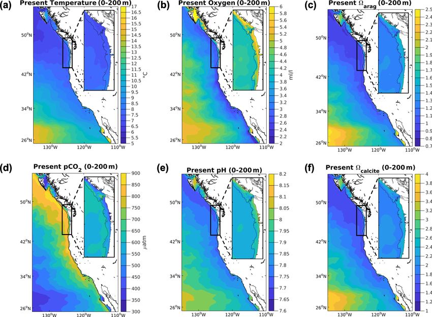
2872        S. A. Siedlecki et al.: Coastal processes modify projected ocean conditions in the California Current System

commonly termed ocean acidification (Caldeira and Wickett,          Time-series due to the upwelling process and is also declin-
2003; Doney et al., 2009; Feely et al., 2004, 2009; Orr et al.,     ing at a slightly faster rate (Chavez et al., 2017). The en-
2005; Sabine et al., 2004). These changing ocean conditions         hanced uptake of CO2 over the CCS shelf amplifies the rate
are occurring in both open-ocean and coastal environments,          of acidification compared to global rates.
where they have the potential to impact marine organisms                Local processes such as upwelling, freshwater delivery,
and ecosystems individually (Doney et al., 2012, 2020; Gat-         eutrophication, water column metabolism, and sediment in-
tuso et al., 2015) and as interactive multi-stressors (Howard       teractions drive biogeochemical variability on regional scales
et al., 2020a; Pörtner et al., 2004; Pörtner and Knust, 2007).      (Cai et al., 2020; Feely et al., 2008, 2016, 2018; Pilcher et
Big changes are happening in the ocean, but there are rea-          al., 2018; Qi et al., 2017; Siedlecki et al., 2017). In the CCS,
sons to believe that global trends may not accurately repre-        winds are critical for upwelling variability and are projected
sent what happens in coastal regions.                               to strengthen in response to global warming (Bakun, 1990;
   The majority of coastal areas have experienced signifi-          Garcia-Reyes et al., 2015; Wang et al., 2015; Rykaczewski
cant increases in sea-surface temperature (SST) at a rate that      et al., 2015; Sydeman et al., 2014). The increased delivery of
exceeds the global average (Hartmann et al., 2013; Lima             O2 -depleted, carbon-rich waters with enhanced nutrients and
and Wethey, 2012). In contrast to most other large marine           increased productivity has been projected for the CCS with
ecosystems, the coastal SST in the California Current Sys-          a global simulation (Rykaczewski and Dunne, 2010). High-
tem (CCS) has decreased over the past 3 decades (Lima and           resolution projections for the CCS reinforced these findings
Wethey, 2012). These results suggest that global projections        (Dussin et al., 2019; Xiu et al., 2018) but projected that
and trends are poor indicators of future change in SST in           the impact of these altered conditions on productivity varied
the CCS and that spatial variability of that change within the      across the CCS, with an increase in the north and a decrease
CCS is also possible.                                               in the south (Xiu et al., 2018), while productivity was iden-
   As the oceans warm, they lose O2 because the solubility of       tified as driving the biggest change in hypoxia in the region
O2 decreases with increasing temperature. However, direct           (Dussin et al., 2019). Howard et al. (2020b) found that, while
solubility effects only partially explain the O2 decline (Bopp      alongshore winds intensified in the future, the upwelling re-
et al., 2013; Breitburg et al., 2018). Warming impacts O2           sponse was dampened by increased stratification. Global pro-
in other ways, for example by raising organismal metabolic          jections have coarse spatial resolution, often having only one
rates and accelerating O2 consumption and by increasing wa-         or two grid cells for the continental shelf, and thus cannot
ter column stratification and thus reducing mixing and venti-       resolve most of the local processes responsible for these ob-
lation (Breitburg et al., 2018; Deutsch et al., 2006). In coastal   served coastal differences.
waters, hypoxic thresholds are more often reached than in               In this paper, we focus on the CCS and its known vulner-
the open ocean because of eutrophication and other local            abilities to climate change by forcing regional models with
processes, such as sediment O2 demand (Diaz and Rosen-              the Coupled Model Intercomparison Project 5 (CMIP5; Tay-
berg, 2008; Rabalais et al., 2010; Siedlecki et al., 2015). In      lor et al., 2012) simulations. We produce multi-model re-
the CCS, hypoxia already occurs regularly on the continental        gionally downscaled climate projections of multiple climate-
shelf (Adams et al., 2013; Connolly et al., 2010; Chan et al.,      associated stressors (temperature, O2 , pH, , and CO2 ) that
2008; Grantham et al., 2004), and continental slope water           resolve coastal processes to create ∼ 100-year projections at
O2 concentrations have been steadily declining for the past         resolutions of 12 and 1.5 km in the northern CCS (N-CCS).
several decades (Bograd et al., 2008; Chavez et al., 2017;          First, we quantify the surface-to-200 m depth-averaged, sea
Deutsch et al., 2011, 2014; Pierce et al., 2012).                   surface, and bottom condition changes for the climate stres-
   Atmospheric carbon dioxide has increased at a rate of            sors projected for 2100 at all resolutions (global, 12 km, and
1–2 ppm yr−1 (Friedlingstein et al., 2019; Le Quéré et al.,         1.5 km). Next, we use the multi-model ensemble to deter-
2018), and surface waters in the open ocean have effectively        mine the degree to which climate-associated stressors are
kept pace with the rising atmospheric concentrations over the       modified relative to global model projections of the CCS con-
last 30 years. Recently, the partial pressure of carbon diox-       sidering this signal both spatially, where the models overlap,
ide (pCO2 ) in coastal shelf waters has been shown in some          and in different regions of the water column representative of
places to lag the rise in atmospheric CO2 , unlike in the open      different habitats. Finally, we interpret our results in the con-
ocean, which implies a tendency for enhanced shelf uptake of        text of previous projections for the CCS and suggest drivers
atmospheric CO2 , with substantial regional variability (Laru-      of the amplification in the downscaled projections by sys-
elle et al., 2018; Cai et al., 2020). One example of regional       tematically comparing the projected changes in the winds,
variability is found in the CCS: over the past 30 years, the        source waters, upwelling strengths, and coastal processes in
CO2 content of waters off the US west coast near Monterey           each model system.
Bay, CA, has increased at a rate greater than that observed
in the open oceans (Chavez et al., 2017). As a result, surface
water pH in Monterey Bay is on average 0.01 units lower
than surface open-ocean measurements at the Hawaii Ocean

Biogeosciences, 18, 2871–2890, 2021                                                    https://doi.org/10.5194/bg-18-2871-2021
S. A. Siedlecki et al.: Coastal processes modify projected ocean conditions in the California Current System                2873

2     Materials and methods                                       2.1.3    1.5 km model

2.1     Model descriptions                                        The highest-resolution (1.5 km) simulations of the N-CCS
                                                                  rely on a modeling framework developed by the University
The downscaled regional modeling frameworks both employ           of Washington Coastal Modeling Group optimized for the
the Regional Ocean Modeling System (ROMS; Shchepetkin             Pacific Northwest “Cascadia” region. The Cascadia model
and McWilliams, 2005). The regional models are forced with        domain encompasses the inland waters of the Salish Sea and
realistic atmospheric and ocean boundary conditions to make       coastal waters of the N-CCS (Fig. 1), and it includes fresh-
hindcast simulations as well as future projections. The model     water and tidal forcing. The grid has a horizontal resolu-
domains are shown in Fig. 1. The downscaled projections           tion of 1.5 km on the shelf, 4.5 km far offshore, and 40 s-
are referred to as “resolving coastal processes” because the      coordinate (terrain-following vertical) levels, with enhanced
historical simulations have been shown to represent observed      bottom and surface resolution. The atmospheric conditions
coastal shelf variability. The model evaluation, provided here    from the 12 km model are used to force the model at this res-
and available in other sources (Davis et al., 2014; Deutsch       olution. The Cascadia model does not simulate biogeochem-
et al., 2021; Giddings et al., 2014; Siedlecki et al., 2015),     istry within the Salish Sea but yields realistic nitrate outflow
indicates the downscaled models perform better spatially and      from the Strait of Juan de Fuca to the outer coast shelf (Davis
temporally (seasonal and interannual) than the global models      et al., 2014). Hindcast experiments from 2004 to 2007 were
for temperature, oxygen, and carbon variables.                    extensively validated and exhibited skill in all regions of the
                                                                  shelf (Davis et al., 2014; Giddings et al., 2014; Siedlecki et
2.1.1    ∼ 1◦ models
                                                                  al., 2015).
These include the CMIP model fields/global-scale model. We
focus here on only the Representative Concentration Path-         2.2     Model metrics
way 8.5 (RCP8.5) from the Earth system models (ESMs)
that make up the CMIP5 modeling framework. The CMIP5              Carbon variables (e.g., pH, pCO2 , and ) were computed
simulations include biogeochemical components described           using model output of DIC, total alkalinity (TA), tempera-
in Bopp et al. (2013). The CMIP models employed here are          ture, and salinity and routines based on the standard OCMIP
further described in Sect. 2.3.                                   carbonate chemistry adapted from earlier studies (Orr et al.,
                                                                  2005) using CO2SYS (Lewis and Wallace, 1998). The total
2.1.2    12 km model                                              pH scale is used for pH throughout.
                                                                     To compute model means and inter-model comparisons,
The mid-resolution (12 km) ROMS-based simulation of the           first a climatological year was generated for each model
CCS is configured for a domain that extends along the North       grid cell, using the years 2002–2004 for the 12 and 1.5 km
American west coast from 25 to 60◦ N and is described in          regional models. Then, annual average values for each
more detail in Howard et al. (2020b). A curvilinear grid is       cell were calculated from the climatology. Finally, spatially
used in the horizontal with close-to-uniform 12 km horizon-       weighted means were calculated from the annual average val-
tal resolution and 33 s-coordinate (terrain-following vertical)   ues. For comparisons between model resolutions, the coarser
levels. Atmospheric conditions including air temperature at       model was interpolated to the higher-resolution model grid.
the sea surface, precipitation, and downwelling radiation are     For example, the global values were interpolated onto the
derived from an uncoupled Weather Research and Forecast-          12 km grid prior to averaging the fields within the CCS. Sur-
ing model output (c3.6.1; Skamarock et al., 2008) as in Re-       face conditions were drawn from the surface vertical layer for
nault et al. (2016a, 2020), with more information in Howard       each simulation. Depth-averaged ocean conditions were cal-
et al. (2020b). To avoid the computational cost of a fully        culated over the upper 200 m for all simulations. Where wa-
coupled ocean–atmosphere model, wind and mesoscale cur-           ter depth was shallower than 200 m, the entire water column
rent feedbacks are parameterized with a linear function of        was averaged. For the bottom comparisons, the global simu-
the surface wind stress as in Renault et al. (2016b). This        lations have a very different bathymetry than the downscaled
linear relationship is supported by observations in the CCS       simulations because of their coarse resolution; consequently
(Renault et al., 2017). The biogeochemical model is detailed      the regional averaging efforts reported here as bottom con-
in Deutsch et al. (2021) and follows Moore et al. (2004).         ditions were isolated to the 0–500 m depth interval only, to
The model has skillfully simulated the recent interannual-to-     ensure that the global model resolved that depth interval. We
interdecadal biogeochemical variability in the CCS (Howard        also report the downscaled values over the shelf only, limit-
et al., 2020b), and a similar model setup forced with data-       ing the determination of metrics out to the 200 m isobath.
assimilated forcing skillfully simulated O2 variability in the       To estimate upwelling intensity, several metrics were
CCS over the last 2 decades (Durski et al., 2017).                employed. The first two rely on the intensity of the
                                                                  winds (e.g., cumulative upwelling index, CUI, Schwing
                                                                  and Mendelssohn, 1997; 8 d wind stress, Austin and Barth,

https://doi.org/10.5194/bg-18-2871-2021                                                   Biogeosciences, 18, 2871–2890, 2021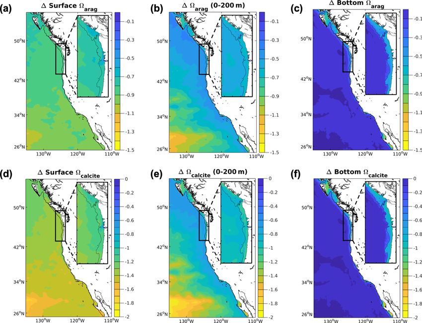
2874         S. A. Siedlecki et al.: Coastal processes modify projected ocean conditions in the California Current System

Figure 1. Base state climate stressor variables in the CCS in both domains. Depth-averaged over 200 m values for the climate stressor
variables in the base state/present conditions for the 12 km (CCS-wide, full panel) and 1.5 km simulations (N-CCS, inset) for (a) temperature
(◦ C), (b) O2 (mL L−1 ), (c) arag , (d) pCO2 (µatm), (e) pH, and (f) calcite .

2002); the third and fourth rely on measures in the water col-           surface energy budget, including net downward shortwave
umn itself and are referred to as the coastal upwelling trans-           and longwave radiation, 10 m wind speed (u and v compo-
port index (CUTI) and biologically effective upwelling trans-            nent), air temperature, and specific humidity. CMIP5 mod-
port index (BEUTI) (Jacox et al., 2018). The wind-based                  els are from the Geophysical Fluid Dynamics Laboratory
metrics, CUI and the 8 d wind stress, are the same for both              (GFDL) (ESM2M), Institut Pierre Simon Laplace (CM5A-
downscaled simulations, but CUTI and BEUTI are specific                  LR), Hadley Centre (HadGEM2-ES), Max-Planck-Institut
to each ocean model as they are calculated based on ocean                (MPI-ESM-LR), and National Center for Atmospheric Re-
measures like vertical transport and nitrate concentrations.             search (NCAR) (CESM1(BGC)). A total of six RCP8.5 sce-
CUTI and BEUTI were integrated over bins of 0.5◦ latitude                nario runs were conducted: one for each individual CMIP5
spanning 0–50 km offshore.                                               model realization and a final run using the five-member en-
                                                                         semble mean forcing. For this paper, we report the output
2.3    Future forcing                                                    from this final ensemble-mean-forced scenario. However, the
                                                                         output from the five individual CMIP5 model realizations
To generate future downscaled projections, the global                    was used to calculate the standard deviation values across
CMIP5 simulations were used to force regional simulations.               the ensemble spread reported in Table 1. Initial and bound-
The methods employed are outlined below.                                 ary conditions had the same kind of centennial trend addition
   The 12 km historical simulation forcing is described in               for temperature, salinity, and all biogeochemical tracers (O2 ,
Renault et al. (2021) and the companion paper, Deutsch                   nitrate, phosphate, silica, iron, dissolved inorganic carbon,
et al. (2021). The 12 km projection was forced by adding                 and alkalinity). More information can be found in Howard et
a monthly climatological difference between the CMIP5                    al. (2020b, Table 1).
RCP8.5 scenario forcing and the historical run forcing, aver-               The 1.5 km projection was forced using the open-ocean
aged over 2071–2100 and 1971–2000, respectively (Howard                  boundary conditions and atmospheric forcing from the 12 km
et al., 2020b), following the delta method commonly ap-                  regional simulation described above (Howard et al., 2020b).
plied in dynamical downscaling and described in Alexander                The boundary conditions included biogeochemical fields
et al. (2020). This is done for all variables that influence the

Biogeosciences, 18, 2871–2890, 2021                                                          https://doi.org/10.5194/bg-18-2871-2021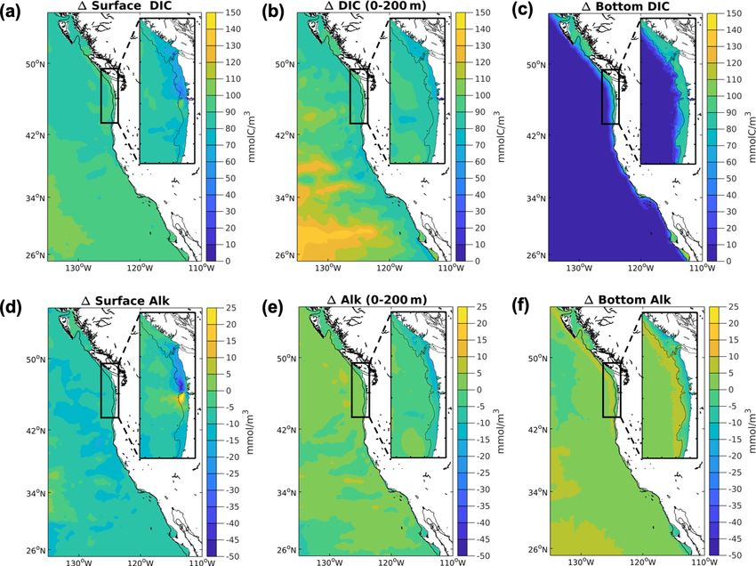
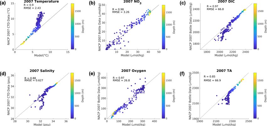
S. A. Siedlecki et al.: Coastal processes modify projected ocean conditions in the California Current System                           2875

Table 1. Annual average differences between climate stressor variables in the future and the base/present conditions for the global ensemble
and 12 and 1.5 km projections over different regions of the water column (200 m averaged, surface, and bottom < 500 m). Column A depicts
the global average from the ensemble average of CMIP5. Column B includes the global (1◦ ) ensemble average difference for the CCS
region followed by, in column C, the CCS-wide difference from the 12 km downscaled results. The final CCS column (column D) includes
the ensemble spread as the range across the five-member model spread of the results for the 12 km model projections column for the CCS
domain. The N-CCS region results span columns E–H in this table. The next three columns detail the differences in the Cascadia domain
for the global ensemble average (column E) and the 12 km (column F) and 1.5 km downscaled projections (column G). The final column
(column H) includes the ensemble spread as the range across the five-member model spread of the results for the 12 km model projections
column for the Cascadia domain. The direction with which each variable described above was amplified/dampened relative to the global
models outside the ensemble variability is highlighted using bold text and dark grey (amplified) and italic text with light grey (dampened)
shading. Within the downscaled simulation, values are also provided just on the shelf (< 200 m isobath) and denoted with an asterisk (*) next
to the number.

from the 12 km model. Because the ecosystem model (BEC)                  ter 1 year of spin-up, a simulation of 2007 was compared
in the 12 km parent grid has more variables than the Casca-              against observations from the region (Fig. 2). The 1.5 km
dia simulation, some of the variables were merged. Specifi-              biogeochemical model skill was similar to the original model
cally, the phytoplankton fields were added together, and the             runs previously published (Davis et al., 2014; Giddings et al.,
nutrients (ammonia and nitrate) were summed into one nitro-              2014; Siedlecki et al., 2015) for 2007 (Fig. 2) without any
gen field. To ensure no biogeochemical model drift between               significant drift in time. Temperature and salinity both expe-
the nested 1.5 km simulation and the 12 km simulation, af-               rienced a significant bias in the upper 200 m in this config-

https://doi.org/10.5194/bg-18-2871-2021                                                           Biogeosciences, 18, 2871–2890, 2021
2876        S. A. Siedlecki et al.: Coastal processes modify projected ocean conditions in the California Current System

uration, unlike the previously published model runs (Fig. 2;      are projected to undergo amplified change. The converse is
temperature RMSE: 2.43; salinity RMSE: 0.627). As we are          referred to as dampening. The ensemble spread is provided
focused on differences between the present day and the fu-        in Table 1 as the range of the five-member model spread of
ture and we expect the bias to remain the same, we do not         the annual average results for the 12 km model projections
bias-correct the forcing here.                                    (columns D and H). The direction with which each variable
   For the future conditions, atmospheric CO2 concentration       described above was amplified relative to the global mod-
(800 ppm) and future atmosphere and ocean forcing from the        els is highlighted using dark grey (amplified) and light grey
12 km runs drove the Cascadia simulations. The river forc-        (dampened) shading in Table 1.
ing was approximated by altering the timing of the freshet
of the 2007 forcing earlier in the year by 2 months. This is
in line with some historical analyses from the N-CCS region       3     Results
(Riche et al., 2014) as well as some projections of future hy-
drological conditions for the Fraser River (Morrison et al.,      Model projections of climate-driven stressor variables (tem-
2002). Both of these results suggest that the total precipita-    perature, O2 , pH, saturation state (), and CO2 ) in each
tion will remain the same, but the increase of rain and de-       downscaled projection were compiled for the CCS for three
crease in snowpack will shift the freshet earlier (Fig. S2 in     depths (200 m averaged, surface, and bottom < 500 m; Ta-
the Supplement). The river TA was not altered from historical     ble 1; Figs. 3–5). The global average changes for many of
forcing, but the rivers equilibrate with the future atmospheric   these variables are different from the 1◦ model projected val-
CO2 concentration (800 ppm).                                      ues for the CCS region, but in only a few cases does this
                                                                  difference fall outside of the ensemble spread reported in
2.4    Future change                                              column D and H of Table 1 (i.e., the signal is amplified or
                                                                  dampened). For each variable and depth, the change between
For each resolution, simulations were run for a number of         the base state and the projected state is described below and
years in a base/present state and then compared to a future       evaluated within the context of the ensemble spread.
simulation. The change is the difference between the future
and base/present state, representing a ∼ 100-year anomaly         3.1    Temperature
due to climate forcing. The historical/base state for the
CMIP5 runs was computed from an ensemble mean spanning            The surface-to-200 m depth-averaged temperatures at all
1971–2000. For the 12 km simulation, the base/present state       model resolutions are consistently warmer in the future CCS,
spanned 1994–2007. For the 1.5 km simulation, the model           both CCS-wide (1.63 and 1.81 ◦ C in the 1◦ and 12 km mod-
was spun up for 1 year (2001), and then the base/present state    els, respectively; columns B and C in Table 1) and within the
spanned 2002–2004. Each level of resolution entails addi-         N-CCS (1.95 to 2.32 ◦ C across the three model resolutions;
tional computer resource costs, which is part of the appeal of    Fig. 3a, columns E–G in Table 1). The Washington shelf ex-
large-scale simulations. The CMIP5 future forcing used here       periences the largest projected differences in the 1.5 km pro-
spans a 30-year mean over 2071–2100. The 12 km model              jection (2.32 ◦ C, Fig. 3). The 1◦ model projected increase for
is a late-21st-century run spanning 2085–2100. The 1.5 km         the CCS (1.63 ◦ C) and the N-CCS (2.21 ◦ C) falls within the
model is also a late-21st-century run spanning 2094–2096.         range of warming from the downscaled projections (CCS:
Results and comparisons for the work presented using both         1.38 to 2.24 ◦ C; N-CCS: 1.55 to 2.35 ◦ C, columns D and H
the 12 and 1.5 km resolution simulations were made using          in Table 1). In both regions of the CCS, the differences be-
the same year span despite runs existing for a broader range      tween the models are smaller than the range of the 12 km
of years for the 12 km simulation. The present state was con-     ensemble (Table 1).
sidered as 2002–2004 for both the 12 and 1.5 km simulations,         At the surface, the SST is warmer in the future in all pro-
and the future was 2094–2096 (Table 1). The global model          jections. Spatially, the SST increases most offshore, and in-
ensemble average results represent a 30-year climatology.         creases least near the coast in all simulations of this east-
                                                                  ern boundary upwelling system, as a result of upwelling
2.5    Modification                                               (Fig. 3b). The 1.5 km model projects slightly smaller in-
                                                                  creases in SST than the 1◦ model or the 12 km model.
The range of the five ensemble members which forced the           However, the 1◦ models project SST increases CCS-wide
12 km projections is used to bound the potential futures ex-      (3.12 ◦ C) and in the N-CCS (3.15 ◦ C), which fall within the
pected. When the differences provided in Table 1 between the      range of SST projections from the 12 km ensemble of down-
mean downscaled conditions for a region of the CCS (CCS-          scaled projections (CCS: 2.57 to 4.05 ◦ C; N-CCS: 2.42 to
wide, columns B and C, or Cascadia/N-CCS, columns E–G)            4.18 ◦ C; columns D and H in Table 1).
and the ensemble spread quantified from the 12 km model              At the bottom, the temperature increases the most near the
projections (columns D and H) both exceed the 1◦ model pro-       coast. The abyssal regions show little to no change in tem-
jected change (columns B and E), those regions of the CCS         perature (Fig. 3c). The shallowest regions of the 1.5 km sim-

Biogeosciences, 18, 2871–2890, 2021                                                 https://doi.org/10.5194/bg-18-2871-2021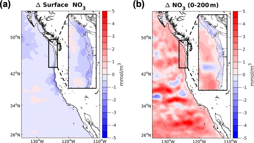
S. A. Siedlecki et al.: Coastal processes modify projected ocean conditions in the California Current System                         2877

Figure 2. Model evaluation. Comparison between the bottle data from the 2007 cruise detailed in Feely et al. (2008) on the y axes and the
simulated parameter (x axis) from the 1.5 km model forced with the 12 km model at the boundaries. Colors indicate the depth where the
bottle sample was taken. Correlation coefficient (R) and root mean squared error (RMSE) are reported as well. The units for each variable
are labeled on the axes.

Figure 3. Projected temperature and oxygen changes in the CCS. Differences between climate stressor variables temperature and oxygen
in the future and the base/present conditions for the 12 km (CCS-wide, full panel) and 1.5 km (N-CCS, inset) projections for (a) SST (◦ C),
(b) depth-averaged temperature over the upper 200 m (◦ C), (c) bottom temperature (◦ C), (d) surface O2 (mL L−1 ), (e) depth-averaged
O2 over the upper 200 m (mL L−1 ), and (f) bottom O2 (mL L−1 ). Positive values indicate a change that is greater in the future than the
base/present condition, and negative values indicate lower values in the future than the base/present conditions depicted in Fig. 1.

https://doi.org/10.5194/bg-18-2871-2021                                                         Biogeosciences, 18, 2871–2890, 2021
2878 S. A. Siedlecki et al.: Coastal processes modify projected ocean conditions in the California Current System
ulation experience the largest warming – nearly 3 ◦ C. In the global projection (Table 1; Fig. 4). The spatial variability
coastal-process-resolving downscaled projections, the pro- within the CCS region differs across resolutions. All pro-
jected bottom temperature change is greater (1.75–1.84 ◦ C, jections show an onshore–offshore gradient in pCO2 with
2.05 ◦ C) than the global projections (1.34–1.65 ◦ C). How- smaller changes closer to the coast and larger changes off-
ever, the 1◦ model projected increases for the whole CCS shore. In the coastal-process-resolving downscaled projec-
(1.65 ◦ C) fall within the range of temperature projections tions, the projected depth-averaged change in pCO2 in-
from the ensemble of 12 km projections (CCS: 1.47 to creases, and the gradient between the nearshore and offshore
2.21 ◦ C; column D in Table 1), while the N-CCS (1.34 ◦ C) intensifies. The 1◦ model projected increase for the CCS
is lower than the range of temperature projections from the (492 µatm) and the N-CCS (527 µatm) falls below the ensem-
ensemble of 12 km projections (N-CCS: 1.40 to 2.10 ◦ C; ble range of downscaled pCO2 projections from the 12 km
columns H in Table 1). model (CCS: 682–836 µatm; N-CCS: 780 to 1066 µatm;
columns D and H in Table 1).
3.2 Oxygen At the surface, future pCO2 consistently increases in all
projections but varies widely across resolutions (Table 1;
Annual depth-averaged O2 concentrations at all model res- Fig. 4). In the downscaled projections, most upwelling areas
olutions consistently decrease in the future compared with experience a smaller increase in surface pCO2 than offshore
the base state, but the magnitude of the decrease is slightly waters. In the 1.5 km projection, regions near the coast of
more severe on average in the downscaled projections (Ta- Oregon show the largest surface pCO2 differences between
ble 1; Fig. 3). The spatial variability within the CCS region, the base and future states, while the region associated with
with more severe declines occurring in the N-CCS, is con- the Columbia River plume shows a much smaller change.
sistent across models but varies in magnitude. The 1◦ model Overall, the inclusion of coastal processes contributes to the
projected decrease for the CCS (−0.52 mL L−1 ) and the N- spatial patterns and magnitudes of projected changes. Con-
CCS (−0.56 mL L−1 ) falls within the range of the ensemble sistent with the subsurface signal, the 1◦ model projected in-
of projections from the 12 km model (Table 1; CCS: −0.52 crease for the CCS (392 µatm) and the N-CCS (365 µatm)
to −0.72 mL L−1 ; N-CCS: −0.52 to −0.92 mL L−1 ; columns falls below the ensemble range of the downscaled projections
D and H in Table 1). from the 12 km model (CCS: 433 to 437 µatm; N-CCS: 424
At the surface, O2 declines in all projections, and the de- to 434 µatm).
gree of change is similar across resolutions (Table 1; Fig. 3), At the bottom, pCO2 is consistently higher in all pro-
consistent with the solubility effect from surface tempera- jections, with varying magnitude across the model resolu-
tures in each simulation. The 1◦ model projected decline falls tions (Table 1; Fig. 4). The range of change in bottom pCO2
within the spread ensemble of projections from the 12 km on the shelf of the 1.5 km projection varies widely (600–
model for the CCS. 1200 µatm), with the most extreme changes occurring on the
The bottom O2 concentration declines in all projections outer shelf and in pockets known to experience persistent hy-
near the coast (Table 1; Fig. 3). The range of change in bot- poxia at present. The 1◦ model projected change for the CCS
tom O2 on the shelf in the 1.5 km projection varies by a fac- (505 µatm) and the N-CCS (592 µatm) falls below the ensem-
tor of 2, with the most extreme changes occurring on the ble range of projections from the 12 km downscaled model
outer shelf and in pockets known to experience persistent hy- (CCS: 650 to 920 µatm; N-CCS: 776 to 1154 µatm).
poxia in the present ocean – e.g., near Cape Elizabeth, south
of Heceta Bank, and within the region associated with the 3.4 pH
Juan de Fuca Eddy (Siedlecki et al., 2015). The 1◦ model
projected decrease for the CCS (−0.43 mL L−1 ) and the N- The pH averaged over 200 m depths for all model resolu-
CCS (−0.63 mL L−1 ) falls within the ensemble range of the tions consistently decreases, and change is less severe than
ensemble of bottom O2 concentration projections from the the global models project for the CCS region (Table 1;
12 km model (CCS: −0.37 to −0.75 mL L−1 ; N-CCS: −0.40 Fig. 4). In the 12 km simulation, a slightly smaller pH change
to −0.92 mL L−1 ; columns D and H in Table 1). When the (∼ −0.26) is observed in the southern CCS than the entire
bottom is restricted to the shelf in the downscaled simula- CCS, within the influence of coastal upwelling. In the 1.5 km
tions (< 200 m isobath; values with asterisk (*) in Table 1), simulation, the regions of largest decline are on the outer
this decrease is more severe but still does not fall outside the shelf and patches of the Oregon shelf. In the downscaled
range from the comparable depth range of the 1◦ model pro- projections, the depth-averaged 200 m pH is lower than the
jection (< 500 m). 1◦ model projected change in the north and greater than
the global change CCS-wide. The 1◦ model projected de-
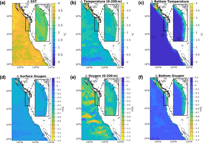
3.3 pCO2 crease for the CCS (−0.321) and the N-CCS (−0.332) falls
within the ensemble range of projections for the downscaled
All model projections of pCO2 consistently increase, with 12 km model (CCS: −0.310 to −0.357; N-CCS: −0.278 to
larger increases in the downscaled projections than in the −0.352).
Biogeosciences, 18, 2871–2890, 2021 https://doi.org/10.5194/bg-18-2871-2021S. A. Siedlecki et al.: Coastal processes modify projected ocean conditions in the California Current System 2879
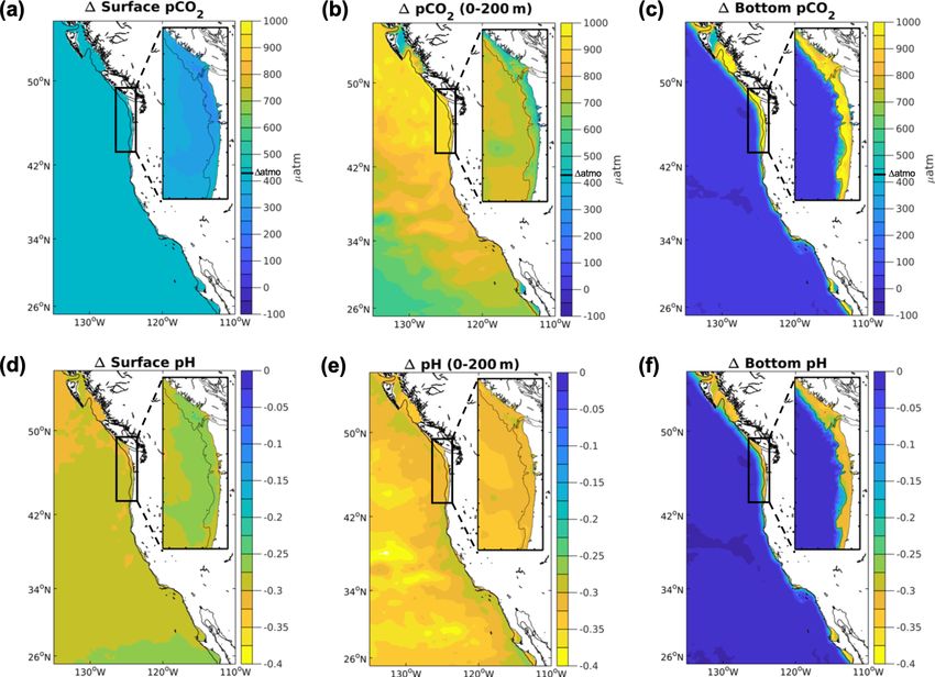
Figure 4. Projected pCO2 and pH changes in the CCS. Differences between climate stressor variables pCO2 and pH in the future and the
base/present conditions for the 12 km (CCS-wide, full panel) and 1.5 km (N-CCS, inset) projections for (a) surface pCO2 (µatm), (b) depth-
averaged pCO2 over the upper 200 m (µatm), (c) bottom pCO2 (µatm), (d) surface pH, (e) depth-averaged pH over the upper 200 m, and (f)
bottom pH. Positive values indicate a change that is greater in the future than the base/present condition, and negative values indicate lower
values in the future than the base/present condition depicted in Fig. 1.
At the surface, the pH consistently decreases in all pro- tions (N-CCS: −0.230 to −0.312) for the downscaled 12 km
jections and is less severe a decrease in the downscaled pro- model.
jections than for the same region in the global model (Ta-
ble 1; Fig. 4). The 1◦ model projected decrease for the CCS 3.5
(−0.319) and the N-CCS (−0.343) is larger than the ensem-
ble range of projections for the downscaled 12 km model
Projections of arag and calcite averaged over 200 m depths
(CCS: −0.285 to −0.287; N-CCS: −0.296 to −0.300).
at all model resolutions consistently decrease in the future,
At the bottom, the pH decreases on the shelf in all pro-
but the magnitude of decrease is usually greater in the down-
jections (Table 1; Fig. 4). In the 1.5 km resolution model,
scaled projections (Table 1; Fig. 5). The projected differ-
the projected conditions show spatial variability on the shelf
ence is greater on the shelf than offshore, but this gradient
that is not apparent in the coarser models. The most se-
is weaker in the 1.5 km projection. The 1◦ model projected
vere changes in bottom pH correspond with regions that
decline in arag for the CCS (−0.71) falls within the ensem-
experience the largest changes in bottom O2 . The down-
ble range of projections for the downscaled 12 km model for
scaled projections indicate decreases in annual average bot-
the CCS (−0.65 to −0.75). The 1◦ projected decline in arag
tom (< 500 m) pH, but spatial variability exists on the shelves
for the N-CCS (−0.62) is larger than the ensemble range of
in the coastal-process-resolving simulations. This difference
projections and larger than the ensemble range of projections
between the 1◦ and downscaled simulations is even greater
for the N-CCS (−0.41 to −0.53) in the downscaled 12 km
on the shelves (indicated as the starred values in Table 1).
model. The same patterns are true for the calcite averaged
The 1◦ model projected decline for the CCS (−0.286) falls
over 200 m depths (Table 1).
within the ensemble range for the downscaled 12 km model
At the surface, consistently decreases in all projections
(CCS: −0.228 to −0.290), while the N-CCS 1◦ model pro-
(Table 1; Fig. 5). Spatially, the 12 km projection shows the
jection (−0.333) is larger than the ensemble range of projec-
largest declines in surface in the southern domain, with
little gradient between the shelf and offshore. At the 1.5 km
https://doi.org/10.5194/bg-18-2871-2021 Biogeosciences, 18, 2871–2890, 20212880 S. A. Siedlecki et al.: Coastal processes modify projected ocean conditions in the California Current System Figure 5. Projected changes in the CCS. Differences between climate stressor variables in the future and the base/present conditions for the 12 km (CCS-wide, full panel) and 1.5 km projections (N-CCS, inset). (a) Surface arag , (b) depth-averaged arag over the upper 200 m, (c) bottom arag , (d) surface calcite , (e) depth-averaged calcite over the upper 200 m, and (f) bottom calcite . Positive values indicate a change that is greater in the future than the base/present condition, and negative values indicate lower values in the future than the base/present condition depicted in Fig. 1. resolution, the N-CCS projected declines are lowest offshore, the range of the ensemble of projections from the downscaled and the declines are even larger than the 12 km projected 12 km model (−0.30 to −0.40). In the 1.5 km model projec- changes even when considering the ensemble spread. The 1◦ tions, the decline is greater than the 1◦ model projects and projected decrease for the CCS (−0.96) is larger than the falls well outside the range of the 12 km projections. This range of the ensemble of projections from the downscaled difference between the global and downscaled simulations is 12 km model (CCS: −0.86 to −0.94). The 1◦ projected de- even greater on the shelves (indicated as the starred values in crease for the N-CCS (−0.76) is smaller or less severe than Table 1). The same is true for the bottom decline in calcite the range of the ensemble of projections from the downscaled (Table 1). 12 km model (N-CCS: −0.82 to −0.88). The same is true for the surface decline calcite (Table 1). 3.6 Themes across projected changes for the CCS At the bottom, decreases in all projections near the coast on the shelves (Table 1; Fig. 5). At the 1.5 km resolution, spa- All climate-associated stressor variables agree with the 1◦ tial variability in the magnitude of the projected conditions projections in terms of the direction of the trend, but not exists on the shelf. The most severe changes in bottom the magnitude of the change. The 1◦ model projections for correspond with regions that experience the largest changes the CCS are largely consistent with the 1◦ model projected in bottom O2 . In the N-CCS, the 1.5 km projected declines global trends, with some differences in the nearshore up- are even larger than the 12 km projected declines even when welling areas (Fig. S1). All carbon variables are sensitive to considering the ensemble range. The 1◦ model projected de- the inclusion of coastal processes, which both downscaled cline in arag for the CCS (−0.47) is more severe than the projections provide. In addition, all of the projections sug- downscaled ensemble range (CCS: −0.38 to −0.46) for the gest greater change in most variables in northern regions of downscaled 12 km model. In the N-CCS, the 1◦ model pro- the CCS and in the upwelling regions. jected decline in arag for the N-CCS (−0.32) falls within Biogeosciences, 18, 2871–2890, 2021 https://doi.org/10.5194/bg-18-2871-2021
S. A. Siedlecki et al.: Coastal processes modify projected ocean conditions in the California Current System               2881

   Nitrate increases over much of the domain in the upper          (0.02) or  (0.03). The majority of the pH and  decline is
200 m (Fig. 6, Table S1 in the Supplement) in both the high-       due to anthropogenic carbon content increase in DIC asso-
and medium-resolution downscaled simulations. Nitrate on           ciated with the RCP8.5 scenario forcing (∼ 95 mmol m−3 ).
average increases in the global simulations, but the magni-        Spatial variability in 1DIC corresponds with variability in
tude and direction vary widely across the ensemble members,        the water buffer capacity and Revelle factor, with southern
a result consistent with Howard et al. (2020b). In addition to     CCS regions of relatively high buffer capacity having the
the projected small increase in nutrient concentrations in the     greatest rates of DIC uptake (Fig. 7, Table S1).
upwelling system of the CCS, the winds are slightly more              TA increases in the future in the subsurface on the shelves
intense (2 % increase in the magnitude of the wind stress)         of the CCS and even more so on the upper slope (Fig. 7,
during the upwelling season (April–September) in the future        Table S1), but it mostly decreases across domains. At the
years. The timing of the onset and duration of the upwelling       surface, it declines, and these two changes offset each other
season in the northern CCS remains the same in the future in       in the depth-averaged 200 m change. Overall, the decrease
these projections. Despite these differences from wind-based       in TA in the projections from the downscaled simulations
upwelling metrics, the in-water upwelling metric CUTI in-          is substantially smaller than the decrease from the 1◦ mod-
dicates no net change in the upwelling intensity of the fu-        els (Table S1). These changes in their corresponding depth
ture N-CCS in the simulations evaluated here. When nitrate         ranges contribute to the results for the carbon variables in
is included in the upwelling measure, as in BEUTI, there is        Table 1, impacting different carbon variables differently; for
a slight decline in the upwelling of nitrate (1–2 %), consis-      example, pCO2 is amplified while pH is not modified over
tent with a decrease in nitrate at the surface in the N-CCS        much of the CCS, and  is amplified at the bottom and the
(Fig. 6). This result is sensitive to the distance offshore (20–   surface but dampened over the upper water column. These
75 km) over which the index is calculated. The direction of        patterns will be examined more closely in Sect. 3.7, which
the trend does not change, but BEUTI, for example, further         focuses on modification and which follows.
declines (4 %) as bin boundaries move closer to shore. The            On the shelves of the downscaled simulations, the source
further offshore the bin extends, the weaker the signal be-        waters are further modified by coastal processes, including
comes. Both of these measures suggest that the upwelling is        increased benthic–pelagic coupling, freshwater delivery, and
not intensified in our projected future, despite the slight in-    denitrification. The inclusion of these processes causes the
crease in winds. This result is consistent with the results of     bottom waters on the shelf to experience a more severe in-
Howard et al. (2020b), where increased stratification in the       crease in pCO2 and declines in oxygen, pH, and  than ob-
future simulations impeded increases in upwelling intensity.       served in the shallowest regions of the global models (starred
   The projected temperature change affects the solubility         values in Table 1). The difference between the bottom esti-
of the gases, generating a solubility-driven decline, and the      mated changes in the CCS in the depth ranges resolved by
increased nutrient content would correspond to a stoichio-         the global models and on the downscaled shelves is greatest
metric oxygen loss as well. Over the entire CCS, the de-           for the carbon variables.
crease in oxygen over the upper 200 m was 0.45 mL L−1 or
20.10 mmol m−3 (Table 1). The solubility-driven change ac-         3.7   Modification
counts for most (∼ 67 %) of this change (13.42 mmol m−3
using 1.92 change in temperature from Table 1). The ad-            In general, the CCS experiences a greater change for most
ditional nitrate brought into the region from the large-scale      variables at all resolutions than the global ocean. However,
models (0.79 mmol m−3 ) corresponds to an additional draw-         only the carbon variables emerge as amplified or dampened
down of 6.81 mmol m−3 of oxygen. In the N-CCS, the                 by the downscaled simulations. Across the spread of ensem-
change in oxygen is a bit larger than across the entire CCS        ble members for the entire CCS in the 12 km simulation, the
– 0.69 mL L−1 (30.82 mmol m−3 , Table 1). The solubility-          downscaled projected increase for pCO2 (columns C, F, and
driven changes contribute a bit less (∼ 44 %) in the N-CCS         G) is amplified relative to the 1◦ models (columns B and E) in
than the entire CCS, but the nitrate signal is larger in the       all three depth ranges (Table 1). The N-CCS pCO2 increase
N-CCS, corresponding to 11.21 mmol m−3 change in oxy-              is amplified in both downscaled simulations (12 and 1.5 km)
gen from an increase of 1.3 mmol m−3 of nitrate in the upper       at all depth ranges (Table 1, columns F and G). In the 200 m
200 m of the water column. The result is that the solubility-      depth-averaged changes, the pCO2 change is correlated to
driven changes combined with the increased supply of nutri-        the TA changes (Table S2). The changes in pCO2 are corre-
ents to the upper 200 m of the N-CCS accounts for 80 % of          lated to the temperature at the surface and to DIC, TA, and
the projected oxygen change in the N-CCS.                          nutrient changes at the bottom (Table S2).
   Similarly, we would expect carbon content to increase              The downscaled decrease in pH at the surface and the bot-
in source waters commensurate with an increase in nutri-           tom is modified relative to what the 1◦ models project for the
ents and lower oxygen concentrations. The corresponding            CCS and N-CCS in the downscaled projections. The surface
stoichiometric increase in DIC to the increase in nutrients        change is less severe than in the 1◦ model and so is consid-
(5 mmol m−3 ) would only account for a small decline in pH         ered dampened relative to global change. At the bottom, pH

https://doi.org/10.5194/bg-18-2871-2021                                                  Biogeosciences, 18, 2871–2890, 2021
2882         S. A. Siedlecki et al.: Coastal processes modify projected ocean conditions in the California Current System

Figure 6. Projected changes in nitrate for the CCS. Differences between the future and the base/present nitrate (NO3 ) conditions for the
12 km (CCS-wide, full panel) and 1.5 km (N-CCS, inset) projections (a) at the surface and (b) depth-averaged (0–200 m). Positive values
indicate a change that is greater in the future than the base/present condition, and negative values indicate lower values in the future than the
base/present condition.

Figure 7. Projected changes for DIC and TA in the CCS. Simulated downscaled changes in annual average DIC and TA (mmol m−3 ) in
the future and the base/present conditions for the 12 km (CCS-wide, full panel) and 1.5 km (N-CCS, inset) projections. (a) Surface DIC
(b), 200 m depth-averaged DIC, (c) bottom DIC, (d) surface TA, (e) 200 m depth-averaged TA, and (f) bottom TA. Positive values indicate a
change that is greater in the future than the base/present condition, and negative values indicate lower values in the future than the base/present
condition.

Biogeosciences, 18, 2871–2890, 2021                                                              https://doi.org/10.5194/bg-18-2871-2021
S. A. Siedlecki et al.: Coastal processes modify projected ocean conditions in the California Current System              2883

in the N-CCS is dampened relative to the 1◦ model. In both       small intensification of about 2 %. The source waters were
downscaled projections (12 and 1.5 km), the surface and bot-     lower, but the oxygen decrease in the N-CCS fell within the
tom pH decrease is dampened in the N-CCS relative to the         range of the ensemble members explored here. Dussin et al.
surface pH decline in the 1◦ model for that region (column       (2019) only explored one global model (GFDL) as a driver,
E). While pH is not modified in the 200 m depth-averaged         and as such the definition of amplification differs from the
changes, at the surface the pH changes are correlated to the     one we use here. Much like experiments conducted by Liu
DIC and TA changes (Table S2).                                   et al. (2012, 2015) for ocean temperatures and described in
   The decrease in  over the upper 200 m is less severe than    Alexander et al. (2020), using a multi-model mean to drive
the 1◦ model projection for the N-CCS and falls outside of       a downscaled ocean model retains the linear component of
the ensemble range, so it is considered dampened relative to     the climate change forcing only and is not able to assess
global change (Table 1). The N-CCS 200 m depth-averaged          the range of the response. Fundamentally, our definition of
 decrease is dampened in both downscaled simulations (12        amplification relies on the range of the ocean condition re-
and 1.5 km) and amplified at the surface (Table 1). At the       sponses. The mechanism of remote biogeochemical redistri-
surface, the changes in saturation state are highly correlated   bution and influence via boundary conditions in the CCS re-
to DIC changes. At the bottom, the changes are also corre-       mains influential for the carbon variables that were identified
lated to the changes in nutrients (Table S2). In the N-CCS       as amplified here. While climate stressor variables have been
region, more of the water column is modified for the carbon      identified as amplified historically using records spanning
variables.                                                       several decades or more (Chavez et al., 2017; Osbourne et
                                                                 al., 2020), regional future projections have focused on multi-
                                                                 model mean conditions projected over 100 years into the fu-
4   Discussion                                                   ture.
                                                                    Although the downscaled model projected a small inten-
Globally, under RCP8.5, the future oceans simulated us-          sification in the projected upwelling-favorable wind stress of
ing CMIP5 are projected on average to be warmer (SST,            2 %, which is consistent with prior work on this topic (Bakun,
mean ± 1SD: 2.73 ± 0.72 ◦ C), higher in pCO2 , lower in O2       1990; Garcia-Reyes et al., 2015; Rykaczewski and Dunne,
content (RCP8.5: −3.45 ± 0.44 %), and more acidified (sur-       2010; Rykaczewski et al., 2015), no change was quantified
face pH: −0.33 ± 0.003 units) (Gattuso et al., 2015). Re-        in the upwelling fluxes in the water column using the CUTI,
gionally, the CMIP5 models project the North Pacific to be       and a slight decline was observed in BEUTI (nutrient flux)
one of the regions to experience the most warming, most se-      measures of upwelling. This is likely due to the compensa-
vere O2 declines, and largest extents of corrosive conditions    tion from increasing stratification in the future simulations
(Bopp et al., 2013; Feely et al., 2009; Gattuso et al., 2015;    as noted in Howard et al. (2020b). We observe lower oxy-
Gruber et al., 2012; Hauri et al., 2013; Long et al., 2016).     gen and higher nutrient content in source waters, but this
Here, we present one of the first downscaled multivariable       change does not make it to the surface. Within the CCS,
projections of environmental change out to the end of the        solubility-driven oxygen changes are important, which is
century in the CCS driven by a suite of CMIP5 forcings in-       consistent with oxygen escape from the ocean being increas-
stead of a single global model. While the downscaled projec-     ingly important in future projections (Li et al., 2020). Moving
tions show changes that are similar in direction to those of     south within the CCS, solubility increasingly outcompetes
the global simulation, the magnitude and spatial variability     nutrient-driven changes in oxygen drawdown. However, the
of the change differ in the coastal-process-resolving down-      projections here indicate that the magnitude of oxygen de-
scaled projections and to a varying degree depending on the      crease was within the bounds of the ensemble range and so
variable, depth range, and subregion of interest.                was not amplified relative to the global models, unlike the
   The CCS experiences a greater change for many variables       carbon variables.
at all resolutions than the global ocean; however this change       The projected change in pH is consistent with prior pH
is modified in the CCS in both downscaled simulations (12        projections for the CCS downscaled with the same RCP8.5
and 1.5 km) for pCO2 , arag and calcite , and pH. Ampli-       scenario using a ROMS model (Gruber et al., 2012; Hauri
fication of global trends within the CCS upwelling systems       et al., 2013; Marshall et al., 2017; Turi et al., 2018). These
in the future has been shown before for oxygen specifically      projections were performed with different biogeochemical
(Dussin et al., 2019) and was identified through the response    models described in Gruber et al. (2012) and Fennel et al.
of the downscaled model to a series of idealized experiments     (2006, 2008) and relied on multi-model means or individ-
with perturbations in the source water oxygen and nutrient       ual ensemble members for the global models. The pH values
concentrations. Source water changes in oxygen drove a 2-        we obtained are lower than the projections of Rykaczewski
fold-larger change in oxygen than nutrient supply alone, and     and Dunne (2010) for the CCS. They used GFDL Earth Sys-
both of these drivers were determined to be more important       tem Model 2.1, a different forcing scenario, and a different
than intensifying winds. In our projections, the more realis-    biogeochemistry model (Dunne et al., 2007). Despite clear
tic winds were different than in Dussin et al. (2019), with a    modification of global trends indicated by downscaled pro-

https://doi.org/10.5194/bg-18-2871-2021                                                 Biogeosciences, 18, 2871–2890, 2021
2884 S. A. Siedlecki et al.: Coastal processes modify projected ocean conditions in the California Current System
jections provided here of pCO2 , , and pH, the biogeochem- the increase in TA modifies the projected pH change in the
ical model formulations differ across resolutions and may be N-CCS by reducing it.
contributing to the amplified signals. Differences include pa- Both biogeochemical models include denitrification at the
rameterizations of gas exchange, detritus classes, sinking ve- sediment water interface, which impacts both the nitrogen
locities, and benthic boundary conditions; the latter has been and TA cycling in the model. Denitrification is a source of
identified in prior work to be important for O2 models in TA (Chen, 2002) and has been shown to impact shelf-wide
coastal regions (Moriarty et al., 2018; Siedlecki et al., 2015). TA in other regions (Fennel et al., 2008). In the CCS, den-
Any of these could contribute to the differences observed itrification has been observed on the shelf and slope, peaks
across model resolutions. CMIP5 results are based on an en- on the slope, and is greater off the Washington coast than
semble average of many models, which all utilize different off Mexico (Hartnett and Devol, 2003). As the source wa-
formulations and complexities for their ecosystem models, ters become lower in oxygen content, denitrification should
further contributing to the uncertainty provided from the bio- increase, providing an additional feedback on the nutrients
geochemical boundary conditions. Overall, the projected an- and carbon variables and dampening the global ocean acid-
nual depth-averaged change in pH appears to depend mostly ification signal. Bottom is not amplified in Table 1, but if
on the anthropogenic forcing scenario, and all the models calculated solely over the shelf region (asterisks in Table 1),
agree on the direction and relative magnitude despite these then bottom changes are amplified in both domains. While
differences. this source of alkalinity has not been observed directly in the
Projected changes in surface and bottom pH, , and pCO2 present-day ocean, a source of TA was identified and inter-
are modified by the inclusion of coastal processes when preted as calcium carbonate dissolution in the CCS (Fass-
downscaling is employed. The variability of carbon variables bender et al., 2011). These results suggest future projections
is influenced by coastal processes in these regions of the wa- should consider salinity and TA forcing feedbacks when per-
ter column. Those processes include the delivery of fresh- forming regional projections as these can alter regional im-
water and sediment–water interactions. At the surface, pH, pacts of carbon variables.
, and pCO2 change differently. TA declines at the surface, Different carbon variables are sensitive to different phys-
while DIC increases. DIC increases due to increased storage ical climate forcings, a result that is consistent with recent
of carbon from the increase in carbon in the future atmo- work suggesting that competing sensitivities may dampen
sphere. The TA changes are driven in part by the altered tim- the variability of pH in the future (Jiang et al., 2019;
ing of the freshet in the N-CCS as well as the presence of a Kwiatkowski and Orr, 2018; Salisbury and Jonsson, 2018;
river plume in an upwelling regime. Freshwater in the region Takahashi et al., 2014). The sensitivities of the various car-
is known to be corrosive due to naturally low TA, which im- bon variables to thermal and geochemical (carbon dioxide)
pacts the buffering capacity of the surface waters. This result forcing were explored in an idealized simulation of future
can be seen in the surface difference plots for pCO2 near the conditions from CMIP5 models in Kwiatkowski and Orr
Columbia River plume (Fig. 4) and the surface TA change (2018), in the present-day ocean in Takahashi et al. (2014)
(Fig. 7). The 12 km projections include climatological fresh- and Jiang et al. (2019), and in the Gulf of Maine by Salisbury
water fluxes as precipitation along the coastline instead of re- and Jonsson (2018). Kwiatkowski and Orr (2018) determined
solving river plumes like the 1.5 km projections, but, despite that the balance between the change in DIC and TA drives the
these different freshwater parameterizations, both models in- variability of pH, in combination with temperature in mid-
dicate modification of carbon variables in the N-CCS Casca- to-high latitudes – effects that largely cancel each other out.
dia domain with different directions for different variables. While the processes that control TA and DIC are similar, the
While the freshwater amplifies the global rate of change for addition of atmospheric CO2 changes DIC alone, altering the
the surface pCO2 and , over the entire water column (200 m balance between these two reservoirs. In the Gulf of Maine,
average), the pH change is dampened as the DIC and TA temperature and salinity anomalies in combination with TA
changes are offset by the temperature changes for that vari- variability offset the long-term ocean acidification trend (Sal-
able. isbury and Jonsson, 2018). Their analysis indicated that is
In our regional downscaled simulations, the changes in more sensitive to temperature and salinity variations than pH,
temperature and TA act together to offset the increase in the and this result was confirmed globally in Jiang et al. (2019).
DIC signal in the coastal upwelling regime (Fig. 7), and for Kwiatkowski and Orr (2018) also found the seasonal ampli-
pH these changes offset each other in the upper 200 m of the tude of arag is expected to strengthen in some regions and
water column. The global models show very little change in attenuate in others due to the high sensitivity of this variable
TA in the region. While the downscaled bottom TA change to temperature.
is small (20–50 mmol m−3 , Fig. 7, Table S1), this amounts to By examining the relationships between the carbon vari-
an increase in pH of 0.07–0.18 and an increase in of 0.15– ables and other regional variables, the relative importance of
0.21 – enough to offset 40–60 % of the reduction in due to different processes responsible for the modification of carbon
increased atmospheric CO2 concentrations. At the bottom, variables by coastal systems can be inferred. Themes emerge
in the correlations with carbon variables across different re-
Biogeosciences, 18, 2871–2890, 2021 https://doi.org/10.5194/bg-18-2871-2021You can also read