Development of a large-eddy simulation subgrid model based on artificial neural networks: a case study of turbulent channel flow - GMD
←
→
Page content transcription
If your browser does not render page correctly, please read the page content below
Geosci. Model Dev., 14, 3769–3788, 2021
https://doi.org/10.5194/gmd-14-3769-2021
© Author(s) 2021. This work is distributed under
the Creative Commons Attribution 4.0 License.

Development of a large-eddy simulation subgrid model based on
artificial neural networks: a case study of turbulent channel flow
Robin Stoffer1 , Caspar M. van Leeuwen2 , Damian Podareanu2 , Valeriu Codreanu2 , Menno A. Veerman1 ,
Martin Janssens1 , Oscar K. Hartogensis1 , and Chiel C. van Heerwaarden1
1 Meteorology  and Air Quality Group, Wageningen University, Wageningen, the Netherlands
2 SURFsara,   Amsterdam, the Netherlands

Correspondence: Robin Stoffer (robin.stoffer@wur.nl)

Received: 26 August 2020 – Discussion started: 10 November 2020
Revised: 14 April 2021 – Accepted: 8 May 2021 – Published: 24 June 2021

Abstract. Atmospheric boundary layers and other wall-            in numeric instability. We hypothesize that error accumula-
bounded flows are often simulated with the large-eddy simu-      tion and aliasing errors are both important contributors to the
lation (LES) technique, which relies on subgrid-scale (SGS)      observed instability. We finally make several suggestions for
models to parameterize the smallest scales. These SGS mod-       future research that may alleviate the observed instability.
els often make strong simplifying assumptions. Also, they
tend to interact with the discretization errors introduced by
the popular LES approach where a staggered finite-volume
grid acts as an implicit filter. We therefore developed an       1   Introduction
alternative LES SGS model based on artificial neural net-
works (ANNs) for the computational fluid dynamics Mi-            Large-eddy simulation (LES) is an often-used technique to
croHH code (v2.0). We used a turbulent channel flow (with        simulate turbulent atmospheric boundary layers (ABLs) and
friction Reynolds number Reτ = 590) as a test case. The de-      other wall-bounded geophysical flows with high Reynolds
veloped SGS model has been designed to compensate for            numbers (e.g. rivers). These turbulent flows are challenging
both the unresolved physics and instantaneous spatial dis-       to simulate because of their strong non-linear dynamics and
cretization errors introduced by the staggered finite-volume     large ranges of involved spatial and temporal scales. LES
grid. We trained the ANNs based on instantaneous flow fields     explicitly resolves only the largest, most energetic turbulent
from a direct numerical simulation (DNS) of the selected         structures in these flows, while parameterizing the smaller
channel flow. In general, we found excellent agreement be-       ones with so-called subgrid-scale (SGS) models. This allows
tween the ANN-predicted SGS fluxes and the SGS fluxes de-        LES to keep the total computational effort feasible for to-
rived from DNS for flow fields not used during training. In      day’s high-performance computing systems but makes the
addition, we demonstrate that our ANN SGS model gener-           quality of the results strongly dependent on the chosen SGS
alizes well towards other coarse horizontal resolutions, es-     model. As an SGS model based on physical principles alone
pecially when these resolutions are located within the range     does not exist, the SGS models used today typically rely on
of the training data. This shows that ANNs have potential to     simplifying assumptions in combination with ad hoc empiri-
construct highly accurate SGS models that compensate for         cal corrections (e.g. Pope, 2001; Sagaut, 2006).
spatial discretization errors. We do highlight and discuss one      To briefly illustrate the effects simplifying assumptions
important challenge still remaining before this potential can    can have, we take as an example the eddy-viscosity assump-
be successfully leveraged in actual LES simulations: we ob-      tion used in the popular Smagorinsky model (Smagorinsky,
served an artificial buildup of turbulence kinetic energy when   1963; Lilly, 1967) and several other SGS models. Crucially,
we directly incorporated our ANN SGS model into a LES            the eddy-viscosity assumption introduces an alignment be-
simulation of the selected channel flow, eventually resulting    tween the Reynolds stress and strain rate tensor that has
                                                                 not been verified in experimental data (Schmitt, 2007). This

Published by Copernicus Publications on behalf of the European Geosciences Union.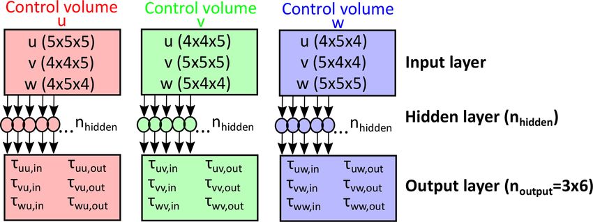
3770                                                                     R. Stoffer et al.: LES subgrid modelling using ANNs

makes it impossible to produce both the correct Reynolds            the Smagorinsky SGS model, neglecting all backscatter) to
stresses and dissipation rates (Jimenez and Moser, 2000).           achieve stable a posteriori results. Such ad hoc adjustments
As a consequence, eddy-viscosity SGS models often require           are not ideally preferred: they obscure the link between the a
ad hoc manual corrections (e.g. tuning the Smagorinsky co-          priori and a posteriori implementation and re-introduce part
efficient and/or implementing a wall-damping function) or           of the assumptions that are ideally circumvented by using
multiple computationally expensive spatial filtering opera-         ANN SGS models.
tions (e.g. scale-dependent dynamical Smagorinsky models               There are also studies that attempted similar methods in
Bou-Zeid et al., 2005) to achieve satisfactory results.             cases that better represent ABLs. Some of them focused on
    Data-driven machine learning techniques are, in contrast,       LES wall modelling specifically (Milano and Koumoutsakos,
much more flexible regarding their functional form and thus         2002; Yang et al., 2019), which is challenging on its own
may potentially help to circumvent the need for many of             because of the many unresolved near-wall motions that the
these simplifying assumptions. This is especially valid for ar-     wall model has to take into account. Sarghini et al. (2003)
tificial neural networks (ANNs): simple feed-forward ANNs           and Gamahara and Hattori (2017), in turn, focused on SGS
with just one hidden layer are theoretically able to represent      modelling in the whole turbulent channel flow. Sarghini et al.
any continuous function on finite domains (i.e. they are uni-       (2003) used neural networks to predict the Smagorinsky co-
versal approximators; Hornik et al., 1989).                         efficient in the Smagorinsky–Bardina SGS model (Bardina
    A wide effort is therefore currently underway to explore        et al., 1980) reaching a computational time savings of about
the potential for ANNs and other machine learning tech-             20 %. Gamahara and Hattori (2017) directly predicted the
niques in flow and turbulence modelling (Brunton et al.,            SGS turbulent transport with a neural network using DNS
2020; Kutz, 2017; Duraisamy et al., 2019). In particular, mul-      during training. They got reasonable a priori results but did
tiple studies successfully modelled turbulence in Reynolds-         not perform an a posteriori test. Another important step to-
averaged Navier–Stokes (RANS) codes with machine learn-             wards application of these methods in realistic atmospheric
ing techniques trained on high-fidelity direct numerical simu-      boundary layers was taken by Cheng et al. (2019). They per-
lations (DNSs) that resolve all relevant turbulence scales (e.g.    formed an extensive a priori test for an ANN-based LES
Kaandorp and Dwight, 2020; Ling et al., 2016a, b; Wang              SGS model covering a wide range of grid resolutions and
et al., 2017; Wu et al., 2018; Singh et al., 2017).                 flow stabilities (from neutral channel flow to very unstable
    Several other efforts in literature experimented with com-      convective boundary layers). We emphasize though that for
parable approaches in both LES SGS modelling (Beck et al.,          successful integration of ANN-based SGS models in practi-
2019; Cheng et al., 2019; Gamahara and Hattori, 2017;               cal applications, accurate and numerically stable a posteri-
Maulik et al., 2019; Milano and Koumoutsakos, 2002; Sargh-          ori results are an important requirement. Recently, Park and
ini et al., 2003; Vollant et al., 2017; Wang et al., 2018; Xie      Choi (2021) took a step in this direction by testing an ANN-
et al., 2019; Yang et al., 2019; Zhou et al., 2019) and, inter-     based SGS model in a neutral channel flow both a priori and
estingly, parameterizations in climate–ocean modelling (e.g.        a posteriori. They found that their SGS model introduced nu-
Bolton and Zanna, 2019; Brenowitz and Bretherton, 2019;             meric instability a posteriori, except when they neglected all
Rasp, 2020; Yuval and O’Gorman, 2020). The studies focus-           backscatter or only used single-point, rather than multi-point,
ing on LES SGS modelling similarly used DNS fields as a             inputs. However, selecting only single-point inputs, in turn,
basis and subsequently applied a downscaling procedure to           clearly reduced the a priori performance. Hence, it remains
generate consistent pairs of coarse-grained fields (that are as-    an open issue whether and how the often-observed high a pri-
sumed to represent the fields that a LES code would gener-          ori potential of ANN SGS models can be successfully lever-
ate) and the quantity of interest (e.g. the “true” subgrid trans-   aged in an a posteriori test, in particular for wall-bounded
port or the closure term itself). These pairs were then typ-        flows like ABLs.
ically used to train ANNs in a supervised way. Some stud-              In addition, all the previously mentioned ANN LES SGS
ies showed very promising results with this method, both in         models, together with traditional eddy-viscosity models, do
so-called a priori (offline) tests (where the predicted quan-       not directly reflect the LES approach where a staggered
tity is directly compared to the ones derived from DNS) and         finite-volume numerical scheme acts as an implicit filter, de-
so-called a posteriori (online) tests (where the trained ANN        spite being a common practice when simulating ABLs. Tra-
is directly incorporated as a SGS model into a LES sim-             ditional eddy-viscosity models are typically derived based
ulation). However, these studies mostly focused on 2-D/3-           on a generic filtering operation that does not consider the
D (in)compressible isotropic turbulence (Beck et al., 2019;         finite discrete nature of the used numerical grid (i.e. it is
Guan et al., 2021; Maulik et al., 2019; Vollant et al., 2017;       usually thought of as an analytical filter like a continuous
Wang et al., 2018; Xie et al., 2019; Zhou et al., 2019) and         top-hat filter), while the ANN SGS models so far did not at-
thus do not represent wall-bounded geoscientific flows. Fur-        tempt to compensate for all the discretization errors arising in
thermore, some of these studies (Beck et al., 2019; Maulik          simulations with staggered finite volumes. These discretiza-
et al., 2019; Zhou et al., 2019) resorted to ad hoc adjustments     tion errors, however, can strongly influence the resolved dy-
(e.g. artificially introducing dissipation by combining with        namics (e.g. Ghosal, 1996; Chow and Moin, 2003; Giaco-

Geosci. Model Dev., 14, 3769–3788, 2021                                             https://doi.org/10.5194/gmd-14-3769-2021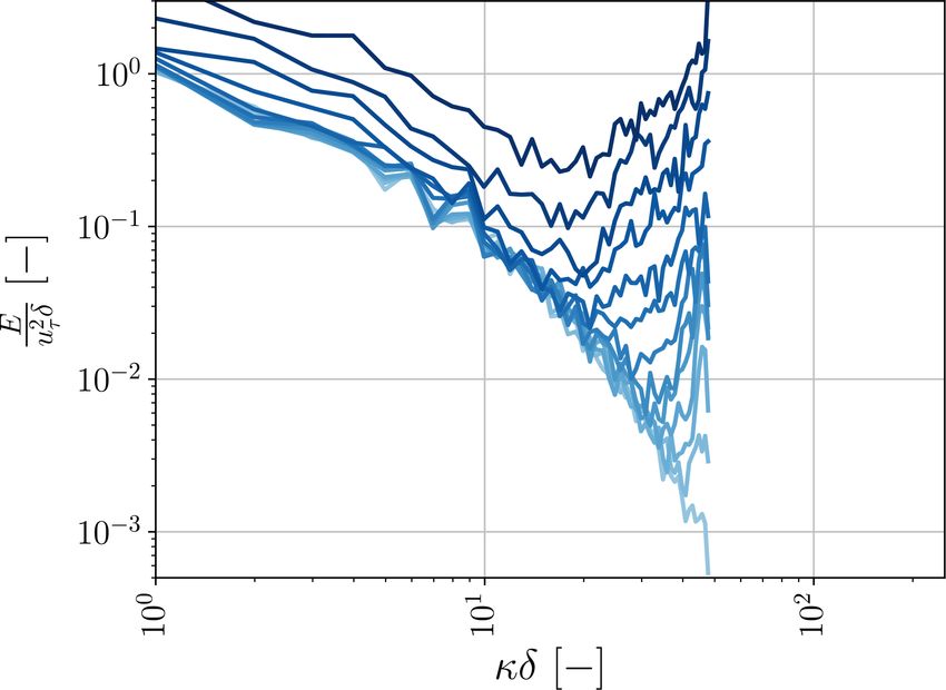
R. Stoffer et al.: LES subgrid modelling using ANNs                                                                             3771

mini and Giometto, 2021), especially at the smallest resolved       2   Theoretical framework of our ANN finite-volume
scales. Since the ANNs have access to both the instantaneous            LES SGS model
DNS flow fields and corresponding coarse-grained field dur-
ing training, a unique opportunity arises to compensate also        As mentioned in Sect. 1, one of our key objectives is to
for instantaneous discretization errors in ANN SGS models.          construct an ANN LES SGS model that compensates for
   Within this context, there have been a couple of note-           the instantaneous discretization errors introduced by implicit
worthy studies (Langford and Moser, 1999; Völker et al.,            filtering with staggered finite-volume numerical schemes.
2002; Zandonade et al., 2004) that introduced the frame-            To derive such an SGS model, we used as a starting point
work of perfect and optimal LES. Based on this frame-               the Navier–Stokes momentum conservation equations for a
work, these studies approximated the full LES closure terms         Newtonian incompressible fluid without buoyancy effects
(that account for both the unresolved physics and all instan-       (which is appropriate for the test case used in this study; see
taneous discretization errors) with a data-driven approach          Sect. 3.1):
based on DNS. The statistical method they used for this
purpose though (i.e. stochastic estimation) still made addi-        ∂uj    ∂ui uj   1 ∂P      ∂ 2 uj
tional assumptions about the functional form of the LES SGS             =−        −        +ν        ,                            (1)
                                                                     ∂t     ∂xi     ρ0 ∂xj    ∂xi 2
model (e.g. linearity). A recent study by Beck et al. (2019)
therefore used ANNs to approximate, in a similar way to the
aforementioned studies, the full LES closure terms. To con-         where uj (u, v, w) [m s−1 ] is the wind velocity along the
struct based on these ANNs an LES SGS model that is nu-             j th direction, t [s] the time, xi and xj [m] the positions in
merically stable a posteriori, they combined the ANNs with          the ith direction and j th direction, respectively, ρ0 [kg m−3 ]
eddy-viscosity models. They did not specifically focus on the       the density, P [Pa] the pressure, and ν [m2 s−1 ] the kinematic
discretization errors associated with staggered finite-volume       viscosity.
grids and did not consider wall-bounded turbulent flows like           The governing LES equations are usually derived by ap-
ABLs.                                                               plying a generic, unspecified filtering operation G to Eq. (1),
   In this study, we therefore made a first attempt to construct,   which introduces a subgrid term τij ≡ ui uj − ui uj that has
based on DNS fields, an ANN SGS model that compen-                  to be modelled (Pope, 2001; Sagaut, 2006). Traditional sub-
sates for both the unresolved physics and the instantaneous         grid models like that of Smagorinsky (Smagorinsky, 1963;
discretization errors introduced by staggered finite-volume         Lilly, 1967) attempt to model τij associated with G. How-
grids. Our ambition in doing so is to eventually improve the        ever, by only considering the generic operation G, they can-
a posteriori accuracy compared to LES with traditional SGS          not directly compensate for the discretization errors aris-
models like the Smagorinsky model. This may potentially re-         ing on a specific finite numerical grid. Although the impact
duce the computational cost involved in LES as well, as ac-         of the discretization errors can be reduced by adopting an
curate results may still be achieved with much coarser, com-        explicit filtering technique (for instance, by increasing the
putationally cheaper resolutions than currently used.               grid resolution compared to the filter width), this is in prac-
   To make a step towards this ambition, our aim with the           tice often not done because of the high computational cost
current paper is two-fold:                                          (Sagaut, 2006). It may therefore be beneficial to develop a
                                                                    LES SGS model that directly compensates for the introduced
  1. We describe the framework of our ANN SGS model,                discretization errors, ideally such that explicit filtering is not
     which takes both the unresolved physics and instanta-          required anymore.
     neous spatial discretization errors in finite-volume LES          To this end, we applied the finite-volume filtering opera-
     into account. This includes its theoretical foundations        tion GFV to Eq. (1) instead of the generic operation G. GFV
     (Sect. 2) and its implementation (Sect. 3).                    is defined as a 3-D top-hat filter sampled on an a priori de-
  2. We characterize both the a priori and a posteriori per-        fined finite-volume grid, where the finite sampling implic-
     formance of our ANN SGS model for a wall-bounded               itly imposes an additional spectral cutoff filter (Langford and
     turbulent neutral channel flow, without resorting to pre-      Moser, 1999; Zandonade et al., 2004). We used GFV to de-
     viously used ad hoc adjustments (Sect. 4). This includes       rive an alternative set of LES equations (Eq. 3) that reflects
     a discussion about the numeric instability we observed         the employed finite-volume grid and removes the need for
     a posteriori (Sect. 4.2), together with suggestions for fu-    commutation between the filtering and spatial differentiation
     ture studies that may help to overcome the observed in-        operators (Eq. 3; Denaro, 2011). This allowed us to explic-
     stability without needing the previously used ad hoc ad-       itly include many instantaneous discretization errors in the
     justments (Sect. 5).                                           definition τij , making use of prior knowledge about the em-
                                                                    ployed finite-volume grid and numerical schemes.
                                                                       Considering for the sake of clarity only equidistant LES
                                                                    grids, following Zandonade et al. (2004), the filtered velocity
                                                                    associated with GFV , uj , at a certain grid cell with indices

https://doi.org/10.5194/gmd-14-3769-2021                                               Geosci. Model Dev., 14, 3769–3788, 2021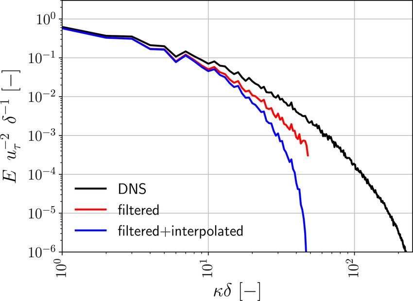
3772                                                                     R. Stoffer et al.: LES subgrid modelling using ANNs

(l, m, n) can be written as                                            To approximate the advection and viscous stress terms on
                   1
                              Z                                     the finite LES grid, in this study, we used second-order linear
uj (l, m, n) =                     uj (x, y, z) dx 0 ,        (2)   interpolations (Sects. 3.2, 4.2). If we then consider specifi-
                 1x1y1z
                          j (l,m,n)                                cally (i) the control volume of the u component and (ii) the
                                                                    transport in vertical direction, we can rewrite the first term
where 1x, 1y, 1z are the equidistant filter widths in the           on the right-hand side of Eq. (3) as follows:
three spatial directions, j (l, m, n) the grid cube/control vol-                  Z
ume for uj at the considered grid cell, and x a vector in-               1                          ∂u
                                                                                            wu − ν        dx 0 dy 0
dicating the position (x, y, z) in the flow domain. Since we        1x1y1z                           ∂z
focused in this study on staggered finite-volume grids (Ta-                    ∂in
                                                                                 u (l,m,n)

ble 1), the location of each control volume j (l, m, n) de-
                                                                                      Z
                                                                        1                                  ∂u
pends on the j component considered (Sect. 3.2).                    −                               wu − ν          dx 0 dy 0
                                                                      1x1y1z                               ∂z
   Applying the finite-volume filter to Eq. (1), using the di-                    ∂out
                                                                                    u (l,m,n)
vergence theorem to convert the volume integrals to surface
                                                                        1 w(l, m, n) + w(l − 1, m, n)
integrals, and combining the advection and viscous stress           =
                                                                       1z                   2
terms, for a certain grid cell, we get an expression similar
                                                                      u(l, m, n) + u(l, m, n − 1)
to that obtained by Zandonade et al. (2004):                        ·
                                  Z                                                 2
∂uj (l, m, n)           1                                               u(l, m, n) − u(l, m, n − 1)
              =−                                                    −ν
      ∂t           1x1y1z                                                             1z
                              ∂j (l,m,n)
                                                                       w(l, m, n + 1) + w(l − 1, m, n + 1)

                         ∂uj
                                                                   −
             · ui uj − ν       ni                                                         2
                         ∂xi                                          u(l, m, n) + u(l, m, n + 1)
                                           Z                        ·
                        1      1                                                    2
             · dx 0 −                            pnj dx 0 ,   (3)
                      1x1y1z ρ0                                         u(l, m, n + 1) − u(l, m, n)
                                       ∂j (l,m,n)                  +ν
                                                                                      1z
where ∂j (l, m, n) is the surface area of the control volume           1  in                out

                                                                    +        τwu (l, m, n) − τwu  (l, m, n) ,                     (4)
j (l, m, n), and ni , nj the ith and j th components, respec-         1z
tively, of the outward-pointing normal vector n correspond-
                                                                    where ∂in                       out
                                                                                 u (l, m, n) and ∂u (l, m, n) are, respectively, the
ing to ∂j (l, m, n). It is noteworthy that, by invoking the
                                                                    lower and upper boundaries of the control volume cor-
divergence theorem, the divergence operator itself is effec-
                                                                    responding to the u component u (l, m, n), representing
tively replaced by surface integrals, which removes the need
                                                                    two different subsets of the total control volume area
for a commutative filter (Denaro, 2011) and avoids the trun-
                                                                    ∂u (l, m, n).
cation errors introduced by the discretization of the diver-             in (l, m, n) and τ out (l, m, n), in turn, are unknown terms
                                                                       τwu                   wu
gence operator on the finite grid.
                                                                    at the lower and upper boundaries of the considered control
   The well-known closure problem does, of course, persist.
                                                                    volume and are directly defined by Eq. (4). They correct for
In fact, none of the terms on the right-hand side of Eq. (3) can
                                                                    the unresolved physics and instantaneous discretization er-
be determined exactly on the available finite LES grid and
                                                                    rors introduced by the employed approximations denoted on
therefore have to be approximated. As argued, however, by
                                                                    the right-hand side.
Langford and Moser (2001) and Zandonade et al. (2004), an
                                                                       The correction terms for the other control volumes and
optimal formulation for the pressure term is impractical and
                                                                    transport components can be defined in a similar manner. In
barely more accurate than traditional finite-volume pressure
                                                                    the remainder of the paper, we will denote the complete cor-
schemes.
                                                                    rection terms with the shorthand notation τijin and τijout . It is
   The errors made in approximating the time derivative, in
                                                                    these complete terms we aim to predict with our ANN-based
turn, are usually constrained by the advection and diffusion
                                                                    LES SGS model. To fully solve Eq. (3), after training, our
terms through the selected time step. Furthermore, the time
                                                                    ANN SGS model only makes use of information available in
discretization scheme we selected (Sect. 3.1) has good en-
                                                                    an actual finite-volume LES: for its inputs, it relies only on
ergy conservation properties with a slight damping of TKE
                                                                    the resolved flow fields u, v, w, and their boundary condi-
over time (van Heerwaarden et al., 2017b).
                                                                    tions (Sect. 3.3).
   In this study, we will therefore only consider the instanta-
neous spatial discretization errors in the advection and vis-
cous stress terms. We further note that, in contrast to eddy-       3   Methodology
viscosity SGS models, the isotropic part of the transport
terms does not have to be incorporated in a modified pres-          In this section, we will describe in detail the implementation
sure term.                                                          of our ANN SGS model. First, we will provide a description

Geosci. Model Dev., 14, 3769–3788, 2021                                              https://doi.org/10.5194/gmd-14-3769-2021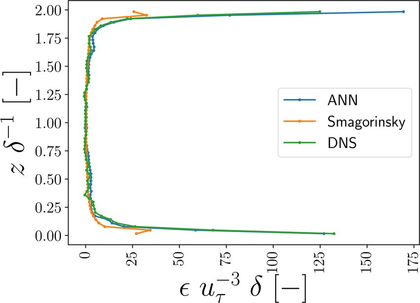
R. Stoffer et al.: LES subgrid modelling using ANNs                                                                             3773

                                                                    3.2   DNS training data generation

                                                                    Using the filtering procedure outlined in Sect. 2, we calcu-
                                                                    lated consistent pairs of (i) low-resolution flow velocity fields
                                                                    uj (that serve as input for the ANN) and (ii) correction terms
                                                                    τijin , τijout (that serve as the ground truth for the ANN predic-
                                                                    tions) from 31 previously stored DNS flow fields (Sect. 3.1).
                                                                    We used these input–output pairs as training data for our
Figure 1. Sketch of simulated turbulent channel flow. Here, δ [m]
                                                                    ANNs (Sect. 3.4).
refers to the channel-half width.
                                                                         By design, the filter in Sect. 2 is directly defined by a se-
                                                                    lected coarse equidistant LES resolution (Eq. 2). To generate
                                                                    the training data, we selected three different typical horizon-
of the DNS test case we used to train and test our ANN SGS          tal equidistant coarse resolutions with an identical coarsening
model (Sect. 3.1). Next, we will briefly outline how we gen-        in the vertical: 192 × 96 × 64, 96 × 48 × 64, and 64 × 32 × 64
erated the data needed to train our ANN SGS model, using            (x × y × z) cells. These three resolutions correspond to hor-
the selected DNS test case (Sect. 3.2). Subsequently, we will       izontal coarse-graining factors, fhor , of 4, 8, and 12, respec-
describe how we designed and trained our ANN SGS model              tively. In the remainder of the paper, we will denote the hori-
(Sect. 3.3 and 3.4). Finally, we will specify how we tested         zontal coarse-graining factor(s) used during training and test-
the a priori and a posteriori performance of our ANN SGS            ing as fhor,train and fhor,test , respectively (see Sect. 3.5.1).
model (Sect. 3.5).                                                       We note that the spatial discretization errors introduced
                                                                    by the applied coarsening, specifically concern errors asso-
3.1   DNS test case                                                 ciated with typically applied second-order linear interpola-
                                                                    tions (Eq. 4). These interpolation errors remove a substantial
We used as a test case a DNS of incompressible neutral chan-        fraction of the turbulent energy remaining after applying the
nel flow (with friction Reynolds number Reτ being equal to          filter (Eq. 2), reflecting their detrimental impact on the small-
590) based on Moser et al. (1999). The friction Reynolds            est resolved scales (Fig. 2). Only by including their impact in
number is a variant of the standard Reynolds number based           the predicted correction terms is our ANN SGS model able
on the friction velocity, which is typically lower in magnitude     to fully compensate for the spatial discretization errors in the
than the standard Reynolds number and is often used in the          advection and viscous stress terms.
context of wall-bounded turbulent flows (e.g. Pope, 2001).
The friction velocity, in turn, is a velocity scale that mea-       3.3   ANN architecture
sures the amount of mechanically generated turbulence and
consequently is a logical scale to consider in neutral channel      We used feed-forward, fully connected ANNs with a sin-
flow. We note that the selected friction Reynolds number is         gle hidden layer to predict the correction terms τijin and τijout
relatively low compared to most turbulent flows occurring in        with the resolved flow fields uj as input. These are sim-
nature.                                                             ple ANNs that facilitate computationally fast evaluations and
   As simulation tool, we used the high-order DNS and finite-       easy implementation. We did not use deeper, more sophisti-
volume LES MicroHH code (v2.0), which has been verified             cated ANNs to limit the computational cost involved in mak-
previously for the case selected in this study (van Heerwaar-       ing predictions with the ANN as much as possible. This com-
den et al., 2017b). The selected neutral channel flow is a tur-     putational cost is critical for the affordability of an ANN SGS
bulent flow bounded by walls at both the bottom and top of          model in an actual LES simulation (Sect. 4.2).
the domain (no-slip boundary conditions), with a mean flow              To introduce non-linearity in the ANN, we used as an acti-
characterized by a symmetric horizontally averaged vertical         vation function the leaky rectified linear unit (ReLu) function
profile (Fig. 1). In the horizontal directions, periodic bound-     (Maas et al., 2013) with the constant α set to the common
ary conditions were applied and a constant volume-averaged          value 0.2. This non-linear activation function, together with
velocity (Uf = 0.11 m s−1 ) was enforced by dynamically ad-         the linear matrix–vector multiplications and bias parameter
justing the pressure gradient.                                      additions, defines the entire functional form of the ANN.
   We stored in total 31 3-D flow fields of the wind veloc-             Similar to conventional LES SGS models, the ANN should
ity fields u, v, and w at time intervals of 60 s after the flow     preferably act on a small subdomain of the full grid to facil-
reached steady state. This time interval was large enough to        itate integration in our simulation code (MicroHH), which
ensure that subsequent stored flow fields were (nearly) inde-       uses domain decomposition for distributed memory com-
pendent, which is preferable for the training and testing of        puting. We consequently predicted with the ANN only the
                                                                      in/out
the neural networks (Sect. 3.4 and 3.5). More details about         τij      values associated with one grid cell (l, m, n) at a time.
the used simulation setup and simulation code can be found          As input to the ANN, we used the locally resolved flow fields
in Table 1 and van Heerwaarden et al. (2017b).                      uj in a 5×5×5 stencil surrounding the grid cell for which we

https://doi.org/10.5194/gmd-14-3769-2021                                               Geosci. Model Dev., 14, 3769–3788, 2021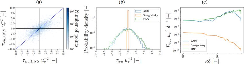
3774                                                                              R. Stoffer et al.: LES subgrid modelling using ANNs

Table 1. Simulation specifications for direct numerical simulation of the incompressible neutral channel flow test case we used to generate
the training data (Sect. 3.2). Here, δ [m] refers to the channel-half width. Additional details about the employed code (MicroHH v2.0) are
given in van Heerwaarden et al. (2017b).

               Friction Reynolds number Reτ                  590
               Boundary conditions                           horizontal directions (x, y): periodic, vertical direction (z): no slip
               Domain size (x, y, z)                         2πδ, πδ, 2δ
               Kinematic viscosity ν                         1.0 × 10⁻⁵ [m2 s−1 ]
               Prescribed volume-averaged velocity Uf        0.11 [m s−1 ]
               Grid resolution (x, y, z)                     768, 384, 256 (stretched in vertical)
               Employed grid                                 staggered Arakawa C grid
               Spatial discretization                        fourth-order interpolation scheme
               Time discretization                           three-stage, third-order Runge–Kutta scheme

                                                                            the flow, potentially removing the need for separate SGS and
                                                                            wall models.
                                                                               Using the 5 × 5 × 5 stencils in combination with the em-
                                                                            ployed staggered Arakawa C grid, an asymmetric bias is in-
                                                                            troduced in the ANN input and output variables if no special
                                                                            care is taken. We overcame this issue by combining three
                                                                            separate single-layer ANNs, where each one corresponded to
                                                                            one of the three control volumes considered (Sect. 2). Here,
                                                                            each received a stencil with slightly adjusted dimensions and
                                                                            predicted only the correction terms (τijin , τijout ) corresponding
                                                                            to the considered control volume (resulting in six outputs per
                                                                            ANN; Fig. 3). This ensured symmetry in the inputs and out-
                                                                            puts of the ANN (Fig. 4a) and did not increase the computa-
                                                                            tional effort involved in evaluating the ANN after training.
                                                                               In fact, this allowed us to reduce the number of ANN eval-
Figure 2. Example stream-wise power spectra of u for the se-                uations in the a posteriori simulation (Sect. 4.2) by almost
lected channel flow (Sect. 3.1) at a height of 0.109δ (i.e. in the          a factor of 2. Except for close to the walls, evaluating the
log layer) and considering a typical coarse equidistant LES reso-           ANN with a checkerboard-like pattern was sufficient to ob-
lution of 64 × 32 × 64 (x × y × z) cells (which corresponds to a hor-       tain all the needed correction terms (Fig. 4b). Close to the
izontal coarse-graining factor of fhor = 8). Here, δ [m] refers to the      walls, we did require (sometimes partial) ANN evaluations
channel-half width. The power spectral density E on the vertical            at every grid cell to calculate all needed correction terms: the
axis has been normalized by δ −1 and uτ −2 , where uτ [m s−1 ] is           checkerboard-like pattern does not provide all the correction
the friction velocity. Here, the black line corresponds to the power        terms at the edges of the domain. In the horizontal directions,
spectrum of the DNS fields, the red line to the power spectrum re-          we could make use of the periodic boundary conditions at the
maining after the finite-volume LES filter (Eq. 2) has been applied,
                                                                            edges of the domain.
and the blue line to the spectrum remaining after both the finite-
volume filter and the second-order linear interpolations required on
the coarse LES grid (Eq. 4).                                                3.4   ANN training

                                                                            We trained the employed ANNs (Fig. 3) using the training
          in/out                                                            data (consisting of corresponding local 5×5×5 uj fields and
predict τij    . Similar to Cheng et al. (2019) and Yang et al.
                                                                                                 in/out
(2019), we opted not to make our inputs Galilean/rotational                 correction terms τij        ; Sect. 3.2) we generated from 31 pre-
invariant as the walls already provide an intrinsic coordinate              viously stored DNS flow fields (Sect. 3.1). The exact number
system and velocity reference.                                              of unique samples we could extract from each flow field dur-
   To select appropriate 5 × 5 × 5 inputs stencils close to the             ing training depended on the considered fhor,train (Sect. 3.2).
boundaries of the domain, we made use of the horizontal                     For the case we mostly focused on in the a priori and a pos-
periodic boundary conditions and the vertical no-slip condi-                teriori tests (i.e. where fhor,train = 8; see Sect. 3.5), we could
tions. We encoded the no-slip conditions in the input stencils              extract 294 912 unique samples from each flow field. Of the
by mirroring uj over the walls, such that uj linearly inter-                31 stored flow fields, we used 25 for training, 3 for validation
polated to the wall was 0 m s−1 . This may have helped the                  during training and tuning of the hyperparameters, and 3 for
ANN to distinguish the near-wall region from the bulk of                    the a priori and a posteriori tests (Sect. 3.5.1).

Geosci. Model Dev., 14, 3769–3788, 2021                                                        https://doi.org/10.5194/gmd-14-3769-2021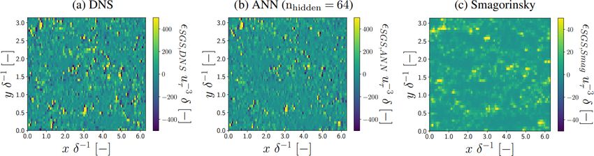
R. Stoffer et al.: LES subgrid modelling using ANNs                                                                                         3775

Figure 3. Architecture of ANN framework used in this study. We combined three separate ANNs that each correspond to one of the three
considered control volumes. For more information, please refer to Sect. 3.3.

Figure 4. (a) Example two-dimensional input stencil of u, v that the ANN corresponding to the control volume of u receives, together
                                in , τ out , τ in , τ out ). (b) Two-dimensional visualization of the way we evaluated the ANN during a posteriori
with four of its outputs (i.e. τuu    uu      uv uv
simulations. By evaluating the ANN in checkerboard-like pattern (i.e. only evaluating the grey-shaded grid cells) and making use of the
periodic boundary conditions, we could calculate all needed correction terms except those close to the walls.

    To train our ANNs, we used TensorFlow (v 1.12.0),                      from the different fhor,train were approximately equally rep-
an open-source machine learning framework (Abadi et al.,                   resented in each training batch.
2016). We relied on the backpropagation algorithm (Rumel-                     Besides that, we implemented preferential sampling near
hart et al., 1986) incorporated within TensorFlow to mini-                 the walls: during training, we selected the five horizontal lay-
mize the loss function. We defined the loss function as the                ers closest to the bottom and top wall more often than the
mean squared error (MSE) between the 18 DNS-derived                        other horizontal layers (starting from the bottom or top wall
  in/out                                                                   towards the centre of the channel, respectively, with a fac-
τij,DNS components (Sect. 3.2) and the 18 ANN-predicted
 in/out                                                                    tor of 10, 8, 6, 4, and 2). The preferential sampling restored
τij,ANN components (Sect. 3.3), combining the results from
                                                                           the balance in the training data set between the physics near
all three separate ANNs (Sect. 3.3). We observed good con-
                                                                           the wall and the bulk of the flow, allowing the ANN to im-
vergence of both the training and validation loss without
                                                                           prove its performance close to the walls where a SGS model
signs of overfitting for all the ANNs we tested (shown as an
                                                                           generally matters most.
example for fhor,train = 8 in Fig. 5).
                                                                              In Table 2, we give an overview of all the hyperparameters
   Here, we chose the popular ADAM optimizer (Kingma
                                                                           and settings we used. The chosen initialization methods for
and Ba, 2014) with a relatively low value for the learning rate
                                                                           the weights and bias parameter are standard for the architec-
η (0.0001) and a relatively large batch size of 1000. As our
                                                                           ture and activation function we selected. Furthermore, in line
training data contain a high amount of noise inherent to tur-
                                                                           with common practice, we normalized all the inputs and out-
bulence, these parameter choices were in our case needed to
                                                                           puts with their means and standard deviations. This improved
stabilize the training results and achieve good convergence.
                                                                           the convergence during training and accelerated learning.
For all the chosen ANNs corresponding to 2 or 3 fhor,train
(see Sect. 3.5.1), we ensured that the samples originating

https://doi.org/10.5194/gmd-14-3769-2021                                                        Geosci. Model Dev., 14, 3769–3788, 2021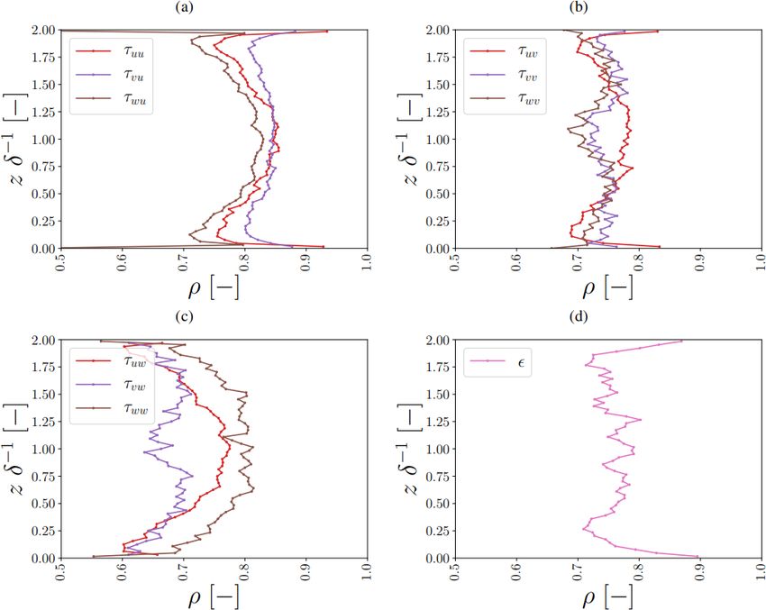
3776 R. Stoffer et al.: LES subgrid modelling using ANNs
Table 2. Fixed hyperparameters and settings used in the ANNs we trained.
No. of training iterations (epochs) 500 000 (≈ 38 epochs for fhor,train = 8, taking into account the preferential sampling)
No. of hidden layers 1
Batch size 1000
Loss function mean squared error, no regularization
Activation function leaky ReLu with α = 0.2(Maas et al., 2013)
Optimizer ADAM with β1 = 0.9, β2 = 0.999, and = 1 × 10⁻⁸ (Kingma and Ba, 2014)
Learning rate η 0.0001
Normalization value−mean )
z score ( standard deviation
Weight/kernel initializer He uniform variance scaling initializer (He et al., 2015)
Bias initializer zeros initializer
3.5 ANN testing
3.5.1 A priori (offline) test
To assess the potential a priori accuracy of our ANN SGS
model, we first compared the ANN predictions to the DNS-
derived values (Sects. 2 and 3.2) for three flow fields held out
during training (Sect. 3.4) and a single representative coarse
LES resolution (i.e. an equidistant grid with fhor,train =
fhor,test = 8; see Sect. 4.1.1). This tests the ability of our
ANN SGS model to generalize towards previously unseen
realizations of the steady state associated with the selected
channel flow (Sect. 3.1).
We especially focused, in the log layer, on τwu and the net
energy transfer towards the unresolved scales, SGS , where
SGS is defined and approximated as SGS ≡ −τij Sij ≈
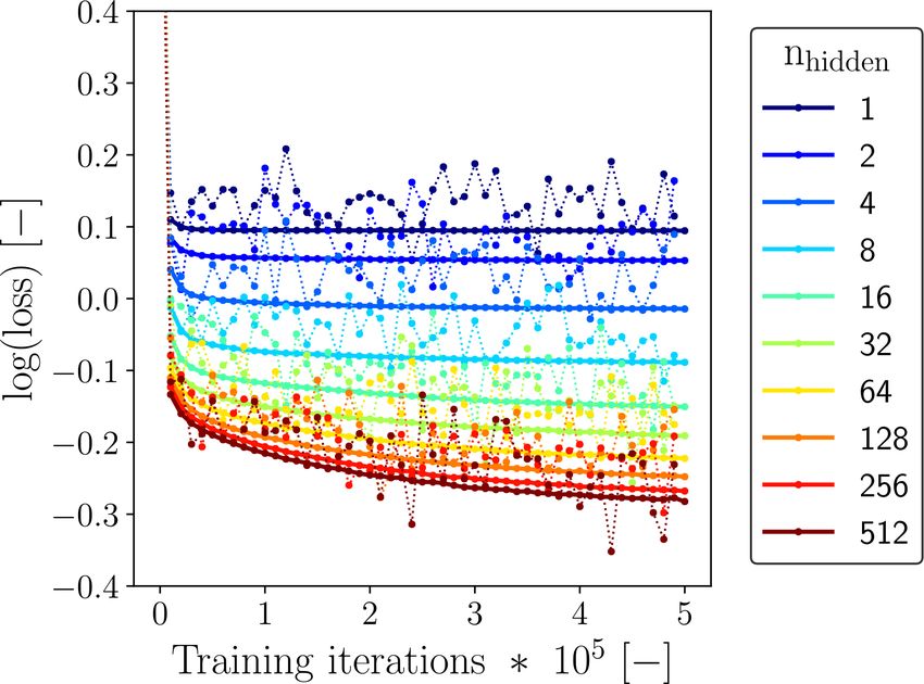
Figure 5. Evolution of the loss corresponding to the considered in/out,int 1uj
training batches (dotted lines) and the three validation flow fields
−τij 1xj . We calculated SGS by interpolating all the
(solid lines) with a changing number of neurons in the single hid- individual components to the grid centres (denoted here as
in/out,int
den layer as a function of training iteration, for the ANNs using τij ) and subsequently summing them. SGS can be both
fhor,train = 8 (see Sect. 3.5.1). To improve readability and keep the positive and negative, where positive values indicate SGS
total computational effort involved in the training feasible, we show dissipation and negative values backscatter towards the re-
here both losses only for every 10 000 iterations instead of every solved scales. Both these processes are critical for the a pri-
single iteration.
ori and a posteriori performance: dissipating sufficient en-
ergy to the unresolved scales is crucial for achieving stable
a posteriori results. τwu , in turn, is also of particular interest
We performed a more extensive sensitivity analysis with
in channel flow: it is the vertical gradient of τwu that has to
the number of neurons in the hidden layer, nhidden , as it is for
balance the imposed horizontal pressure gradient (e.g. Pope,
our architecture a good measure of the model complexity. In
2001), making τwu critical for the quality of the achieved
general, we found for all three selected fhor (Sect. 3.2) that
steady-state solution. The log layer is mainly interesting be-
increasing nhidden , and thus increasing the model complexity,
cause of its universal character. In the log layer, the horizon-
improved the reduction of the loss function without show-
tally averaged profiles of the mean velocity and Reynolds
ing signs of overfitting (shown as an example for fhor = 8
stress tensor components become partly independent of the
in Fig. 5). However, the improvement in training loss reduc-
Reynolds number when properly scaled with wall units (e.g.
tion clearly reduced with increasing model complexity, while
Pope, 2001).
a higher model complexity increases the computational cost
As a reference, we included in the comparison the sub-
of the ANN SGS model. In the next sections, we will there-
grid fluxes and net SGS transfer predicted with the popu-
fore focus on the results we obtained with nhidden = 64, as a
lar Smagorinsky (Lilly, 1967) SGS model (see Sect. 4.1.2),
reasonable compromise between accuracy and total compu-
which we will denote as τij,Smag and smag , respectively.
tational cost.
In the Smagorinsky SGS model, τij,Smag is modelled as
τij = −2νr Sij , with νr being the modelled eddy-viscosity
coefficient and Sij being the filtered strain rate tensor (de-
Geosci. Model Dev., 14, 3769–3788, 2021 https://doi.org/10.5194/gmd-14-3769-2021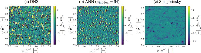
R. Stoffer et al.: LES subgrid modelling using ANNs                                                                             3777

                     ∂ui    ∂uj
fined as Sij ≡ 12 ∂x   j
                         +  ∂xi ) (Pope, 2001, e.g.). In line          feature importance measures by which factor the prediction
with usual practice for wall-bounded flows, we augmented               error (in our case measured as the root mean square error
the model for νr with an ad hoc Van Driest (Van Driest,                between the DNS values and ANN predictions) increases
1956) wall-damping function to (partly) compensate for the             when the information contained in that input variable is de-
known over-dissipative behaviour close to walls (e.g. Pope,            stroyed, while the information in the other input variables is
2001; Sagaut, 2006). Consequently, νr is effectively mod-              retained. We destroyed the information in each input vari-
elled as νr = cs 1 1 − exp −z+ /A+
                                          2
                                               S, with cs being        able by randomly shuffling it in the corresponding horizontal
the Smagorinsky coefficient (which is being set to 0.1), 1             plane. Besides that, we averaged the calculated permutation
                                                      1                feature importances over all three testing flow fields and over
being the filter size (defined as 1 ≡ (1x1y1z) 3 ), z+ the
                                                                       10 different random shufflings to stabilize the results. We in-
absolute vertical distance from the closest wall normalized
                                                                       tentionally chose not to shuffle the input variables along dif-
by u∗ and δ, A+ an empirical constant (which is being set to
                                                                       ferent heights. Because of the strong mean vertical gradient
26), and S the squared filtered strain rate tensor (defined as
              1                                                       in u, this would possibly introduce an unrealistic bias into
S = 2 Sij Sij 2 ).                                                     the calculated permutation feature importances. We do em-
   To facilitate easier interpretation and comparison with the         phasize that the permutation feature importances are likely
Smagorinsky SGS model, for the ANN and DNS results, we                 affected by the correlations existing in our input data. The
combined the two separate correction terms τijin , τijout . In the     permutation feature importances we report therefore need to
remainder of the paper, we will denote the resulting com-              be interpreted with caution.
bined correction terms as τij,ANN and τij,DNS , where both
consist of the same nine components as τij,smag . We did this
in accordance with the way we evaluated the ANNs within                3.5.2   A posteriori (online) test
our computational fluid dynamics (CFD) MicroHH code dur-
ing the a posteriori test (Sect. 3.3).                                 To test the a posteriori performance of our ANN LES SGS
   On top of the comparison for a single coarse horizontal             model, we directly incorporated one of our ANNs (i.e. with
resolution, we separately explored the generalization perfor-          nhidden = 64 and fhor,train = 8) into our CFD code (Mi-
mance of the developed ANN SGS model with respect to the               croHH v2.0) (van Heerwaarden et al., 2017b). We chose the
selected coarse horizontal resolution in Sect. 4.1.3 . To this         input and output variables of our ANN SGS model such that
end, we trained our ANN SGS model, in three different ways,            the integration into our CFD code was relatively straightfor-
on filtered DNS data corresponding to all selected fhor (4, 8,         ward (Sect. 3.3). Furthermore, we improved the computa-
and 12, respectively; see Sect. 3.2):                                  tional performance of the ANN SGS model by implement-
                                                                       ing basic linear algebra subprogram (BLAS) routines from
  1. train only on filtered DNS data corresponding to fhor =           the Intel® Math Kernel Library (version 2019 update 5 for
     8,                                                                Linux), which has been optimized for the Intel CPUs we used
                                                                       (i.e. E5-2695 v2 (Ivy Bridge) and E5-2690 v3 (Haswell)).
  2. train on filtered DNS data corresponding to fhor = 4, 12,
                                                                       Still, the computational effort involved in the ANN SGS
     and
                                                                       model was large: an equivalent LES simulation with the
  3. train on filtered DNS data corresponding to all three             Smagorinsky SGS model was for our setup about a factor
     fhor .                                                            of 15 faster, showing that, in its current form, our ANN SGS
                                                                       model still needs more optimizations for practical applica-
For all three training configurations mentioned above, we              tions.
tested the performance of the ANN SGS models on previ-                    With the ANN SGS model incorporated in our CFD code,
ously unseen filtered data corresponding to all three fhor .           we ran a LES with an equidistant grid of 96 × 48 × 64 cells,
This thus includes several cases where the ANN SGS model               directly corresponding to the selected fhor,train = 8, for the
is being applied to other resolutions than seen during train-          turbulent channel flow test case described in Sect. 3.1. Here,
ing.                                                                   we used second-order linear interpolations to calculate all the
   Finally, to get some more insight into the behaviour of our         velocity tendencies, consistent with our filtering and train-
ANNs, in Sect. 4.1.4, we calculated for every input variable           ing data generation procedure (Sect. 2 and 3.2). Furthermore,
in the 5 × 5 × 5 stencils the so-called “permutation feature           we initialized the LES simulation from one of the three flow
importance” (e.g. Fisher et al., 2019; Molnar, 2019; Breiman,          fields reserved for the a priori testing. We did this to ensure
2001) associated with predicting τwu  in and τ out in the log layer.   that any possible errors in the initialization phase of the LES
                                               wu
   The most important advantage of these “permutation fea-             (i.e. before steady state is achieved) did not impact the solu-
ture importances” is their intuitive meaning: they indicate            tion. Still, our LES ran freely from the prescribed initialized
how important a certain input variable is for the prediction           steady-state fields, meaning that all the model and discretiza-
                 in , τ out in the log layer: the higher it is, the
quality of the τwu                                                     tion errors made in calculating the channel flow steady-state
                       wu
more important that variable is. Specifically, the permutation         dynamics were included.

https://doi.org/10.5194/gmd-14-3769-2021                                                 Geosci. Model Dev., 14, 3769–3788, 2021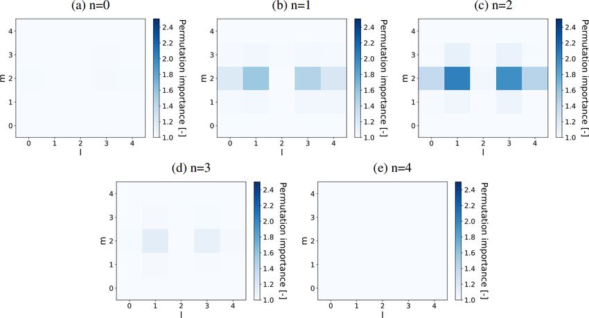
3778                                                                      R. Stoffer et al.: LES subgrid modelling using ANNs

4     Results and discussion                                         sisted even when the errors were weighted inversely propor-
                                                                     tional to their probability density function (PDF) (i.e. giving
In this section, we will characterize the a priori and a pos-        extreme values larger weights in the loss function).
teriori performance of our ANN SGS model. We will first                 Extending our focus from the log layer to vertical pro-
describe the a priori performance of our ANN SGS model               files of horizontally averaged τwu and SGS , in general, we
and the Smagorinsky SGS model for a single coarse res-               again observe quite good correspondence between the ANN
olution (i.e. where fhor,train = fhor,test = 8; Sect. 4.1.1 and      predictions and DNS-derived values (Figs. 10 and 11). In
4.1.2). Subsequently, we will discuss the generalization per-        the profile of τwu,ANN , we do see some deviations from the
formance of our ANN SGS model with respect to the selected           τwu,DNS profile, especially close to the walls. In our training
coarse resolution (Sect. 4.1.3) and the permutation feature          data, the horizontally averaged flux of τwu,DNS was generally
importances associated with the input stencils (Sect. 4.1.4).        small compared to its point-wise fluctuations. As a result, the
Finally, we will describe and discuss the instability we ob-         loss associated with τwu,DNS was probably more sensitive to
served a posteriori (Sect. 4.2).                                     the point-wise fluctuations than the average flux, which may
                                                                     have contributed to the observed deviations.
4.1     A priori (offline) test                                         The vertical profile of SGS,ANN , in turn, matches very
                                                                     closely the profile of SGS,DNS . The ANN approximately pro-
4.1.1    Single horizontal-resolution ANN performance                vides the net dissipation inferred from the DNS, which pri-
                                                                     marily occurs close to the walls. Hence, this does not make
The ANN-predicted τwu,ANN , SGS,ANN (with nhidden = 64;             yet clear why our ANN SGS model induces the observed a
see Sect. 3.4) values in the log layer generally show excellent      posteriori instability. In Sect. 4.2, we will elaborate more on
agreement with the DNS-derived values (Figs. 6–9). Espe-             potential reasons why our ANN SGS model nonetheless in-
cially the consistency we found in the horizontal cross sec-         duces instability.
tions (Figs. 6a and b, 7a and b) is striking given the noisy            Extending our focus towards all components, we found
spatial patterns of τwu,DNS and SGS,DNS , which the ANN             that in general the ANN correlated well with all DNS-derived
reproduces quite accurately both qualitatively and quantita-         correction and SGS transfer terms (third row in Table 3 and
tively. Particularly noteworthy is its ability to accurately re-     Fig. 12; mostly ρ = 0.6–0.9). Looking more closely at the
produce both negative and positive SGS,DNS , as these are as-       found correlations, we did find that the correlations differed
sociated with backscatter and SGS dissipation, respectively.         depending on the channel height. Closer to the walls, the cor-
These two processes are both critical for the quality of the a       relations generally slightly decreased compared to the middle
posteriori simulations (see Sect. 4.2).                              of the channel (except for the vertical layers directly adja-
   We note that the found correspondence between correction          cent to the wall, where most terms show a better correlation).
and SGS transfer terms in the log layer of neutral channel           Here, we emphasize that we implemented a preferential sam-
flow is in agreement with the results of Cheng et al. (2019),        pling technique (Sect. 3.4), which helped to minimize this
Park and Choi (2021), and Gamahara and Hattori (2017), de-           reduction of prediction performance close to the walls com-
spite our training data generation procedure additionally ac-        pared to the middle of the channel.
counting for numerical errors associated with LES where a               Looking at the individual terms, some of them were clearly
staggered finite-volume grid acts as an implicit filter (Sects. 2    better predicted than others (e.g. τvu vs. τvw ): this was likely
and 3.2). Consistent with the matching horizontal cross sec-         related to differences in their magnitude that persisted even
tions, the ANN reproduces quite well the distributions and           after the applied normalization (i.e. the same normalization
spectra of τwu,DNS and SGS,DNS (Figs. 8b and c, 9b and c).          was applied over the entire domain, meaning that some com-
The notable high normalized spectral density of τwu,DNS at           ponents with strong vertical gradients still contained more
high wave modes is a direct consequence of the instantaneous         extreme values than components without a clear vertical gra-
spatial discretization errors we compensate for. As these dis-       dient) and differences in their stochastic variability and con-
cretization errors remove a large part of the variance at the        sequent signal-to-noise ratio.
smallest resolved spatial scales (Fig. 2), the corresponding            One clear outlier is τwu at the first vertical level (with
correction terms, including τwu , are characterized by strong        ρ = 0.339; not shown), which appeared to be most difficult
variability at the smallest resolved scales.                         to predict. This component was located at the bottom wall
   From the tails of the distribution and the high wave modes        because of the staggered grid orientation and consequently
of the spectra (Figs. 8b and c, 9b and c), it is apparent that the   only the viscous flux contributed. As a consequence, the tar-
ANN does still slightly underestimate the extremes at small          get DNS values and input patterns were different than for
spatial scales characteristic of τwu,DNS and SGS,DNS . Proba-       other vertical levels and components, making it hard for the
bly, these extremes were hard to predict accurately because          ANN to give accurate predictions. Still, the magnitude of the
of their high stochastic nature and inherent rare occurrence.        ANN predictions matched the DNS values reasonably well
Yang et al. (2019) identified this issue in the context of an        (not shown).
ANN-based LES wall model and found that this issue per-

Geosci. Model Dev., 14, 3769–3788, 2021                                               https://doi.org/10.5194/gmd-14-3769-2021
R. Stoffer et al.: LES subgrid modelling using ANNs 3779
.
Figure 6. Horizontal cross sections of τwu in the log layer (0.09375 δz (55.3125z+ )) for a representative flow field not used to train and
validate the ANNs. All values are normalized by the friction velocity uτ and half-channel width δ.
.
Figure 7. Horizontal cross sections of SGS in the log layer (0.109375 δz (64.53125z+ )) for a representative flow field not used to train and
validate the ANNs. All values are normalized by the friction velocity uτ and half-channel width δ.
4.1.2 Single horizontal-resolution Smagorinsky SGS,smag is smaller and skewed towards low wave modes
performance (Figs. 8c and 9c).
This exacerbated point-wise a priori performance of the
Considering the individual grid points, the a priori perfor- Smagorinsky SGS model is caused by our alternative defini-
mance of the Smagorinsky SGS model is in sharp contrast tion for τij , which, in contrast to the commonly defined τij ,
with the a priori ANN performance: τij,smag , and to a some- compensates for all the instantaneous discretization effects
what lesser extent SGS,smag , shows barely any agreement introduced by the staggered finite volumes in both the advec-
with the DNS-derived values both qualitatively and quantita- tion and viscous flux terms (Sect. 2). As these discretization
tively (Figs. 6–9). The poor point-wise a priori performance effects remove a large part of the variance present in the LES
of Smagorinsky is well known in literature (e.g. Clark et al., (Fig. 2), our τij inherently contains a large amount of vari-
1979; McMillan and Ferziger, 1979; Liu et al., 1994). In ad- ance that is not represented by Smagorinsky.
dition, we can also observe its known inability, in the form Focusing on the horizontally averaged vertical profiles of
we employed, to account for backscatter (e.g. Pope, 2001; τwu , we consequently found also that τwu,smag does not com-
Sagaut, 2006). pare well with τwu,DNS (Fig. 10). Except close to the walls
In our case though, the point-wise a priori performance and the centre of the channel, the Smagorinsky SGS model
of Smagorinsky is still worse than usually documented: the strongly underestimates the horizontally averaged τwu . We
found correlations with DNS in our study (mostly ρ = 0.0 at emphasize that the correspondence close to the walls was
individual heights for all correction and dissipation terms; only achieved because of the implemented ad hoc Van Driest
not shown) are lower than reported before (where ρ =∼ wall damping function (Van Driest, 1956).
0. . .0.4; Cheng et al. (2019); Clark et al. (1979); McMil- In the horizontally averaged vertical profiles of SGS
lan and Ferziger (1979); Liu et al. (1994)). Furthermore, (Fig. 11), we observe a striking characteristic that may seem
τwu,Smag and SGS,smag are off by approximately 1 order of counterintuitive at first: the Smagorinsky SGS model un-
magnitude and are too smooth (Figs. 6, 7 and 8–9b and c): derpredicts SGS,DNS at the walls, despite its known over-
in comparison to τwu,DNS and SGS,DNS , the PDF is nar- dissipative behaviour in a posteriori tests (e.g. Pope, 2001;
rower (Figs. 8b and 9b), and the spectral energy in τij,Smag ,
https://doi.org/10.5194/gmd-14-3769-2021 Geosci. Model Dev., 14, 3769–3788, 20213780 R. Stoffer et al.: LES subgrid modelling using ANNs
Figure 8. Performance of τwu,ANN (with nhidden = 64) in the log layer (0.09375 δz (55.3125z+ )) for a representative flow field not used
to train and validate the ANNs. Panel (a) shows the corresponding hexbin plot between τwu,ANN and τwu,DNS , where the dotted blue line
indicates the 1 : 1 line. Panel (b) shows the probability density functions and panel (c) the stream-wise spectra averaged in the span-wise
direction. τwu,ANN and τwu,DNS have been normalized by the friction velocity u−2 τ . The power spectral density E on the vertical axis in
panel (c) has been normalized by δ −1 and uτ −2 . As a reference, in panels (b) and (c), τwu,smag is shown as well.
Figure 9. Performance of SGS,ANN (with nhidden = 64) in the log layer (0.109375 δz (64.53125z+ )) for a representative flow field not used
to train and validate the ANNs. Panel (a) shows the corresponding hexbin plot between SGS,ANN and SGS,DNS , where the dotted blue line
indicates the 1 : 1 line. Panel (b) shows the probability density functions and panel (c) the stream-wise spectra averaged in the span-wise
direction. SGS,ANN and SGS,DNS have been normalized by the friction velocity u−3 τ and δ. The power spectral density E on the vertical
axis in panel (c) has been normalized by uτ −3 . As a reference, in panels (b) and (c), SGS,Smag is shown as well.
Figure 10. Vertical profiles of horizontally averaged τwu,DNS , Figure 11. Vertical profiles of horizontally averaged SGS,DNS ,
τwu,ANN , and τwu,smag at one representative time step not used SGS,ANN , and SGS,smag at one representative time step not used
to train and validate the ANNs. All values are normalized by the to train and validate the ANNs. All values are normalized by the
friction velocity u−2 −1
τ and half-channel width δ . friction velocity u−3
τ and half-channel width δ.
Geosci. Model Dev., 14, 3769–3788, 2021 https://doi.org/10.5194/gmd-14-3769-2021R. Stoffer et al.: LES subgrid modelling using ANNs 3781
Figure 12. Vertical profiles of correlation coefficients between ANN predictions and DNS values for all correction and dissipation terms (a–
d) at one representative time step not used to train and validate the ANNs. Here, the j index refers to the considered control volume (Sect. 2).
The heights are normalized by the half-channel width δ −1 . Note that the τuw,vw components are left out at the first vertical level, as these
are due to the staggered grid located exactly at the bottom wall. At the bottom wall, we imposed a no-slip boundary condition, meaning that
these components are by definition 0.
Sagaut, 2006). However, as the Smagorinsky SGS model 4.1.3 Multiple horizontal-resolution ANN
does not directly compensate for instantaneous discretization generalization
errors (and thus does not re-introduce the associated inherent
variance), the Smagorinsky SGS needs to produce less dissi- Overall, our ANN SGS model shows promising generaliza-
pation than our ANN SGS model to achieve stable a posteri- tion capabilities towards other coarse horizontal resolutions
ori results (see also Sect. 4.2). than the one considered in the previous section. The extent to
All in all, our ANN SGS model is clearly better able to which it is able to maintain its high a priori accuracy, how-
represent τij,DNS and SGS,DNS in the presented a priori test ever, does strongly depend on the considered ftrain,hor and
than the Smagorinsky SGS model. This shows the promise ftest,hor (Table 3).
ANN SGS models like ours could have to construct more ac- Considering first the ANNs solely trained on fhor,train = 8
curate SGS models that, in contrast to traditional SGS mod- (rows 2–4 in Table 3), we find, unsurprisingly, that they
els like Smagorinsky, additionally compensate for instanta- achieve their best performance when fhor,test = 8 (which is
neous spatial discretization errors. The most important issue identical to the configuration used in Sect. 4.1.1). More in-
remaining, is whether and how this a priori potential can be terestingly, however, we observe that these ANNs already
successfully leveraged in a posteriori simulations without in- have some generalization capability, even without having
troducing numeric instability. seen multiple fhor,train . This does depend on the selected
fhor,test : the performance is better for fhor,test = 12 than for
fhor,test = 4 (where for multiple terms ρ < 0.5; not shown).
Comparing these ANNs to the ones trained on fhor,train =
4, 12 (rows 5–7 in Table 3), first of all, we see a clear, un-
surprising improvement when fhor,test = 4, 12: including the
https://doi.org/10.5194/gmd-14-3769-2021 Geosci. Model Dev., 14, 3769–3788, 2021You can also read