Efficient Bayesian inference for large chaotic dynamical systems
←
→
Page content transcription
If your browser does not render page correctly, please read the page content below
Geosci. Model Dev., 14, 4319–4333, 2021
https://doi.org/10.5194/gmd-14-4319-2021
© Author(s) 2021. This work is distributed under
the Creative Commons Attribution 4.0 License.

Efficient Bayesian inference for large chaotic dynamical systems
Sebastian Springer1,2 , Heikki Haario1,3 , Jouni Susiluoto1,3,4 , Aleksandr Bibov1,6 , Andrew Davis4,5 , and
Youssef Marzouk4
1 Department  of Computational and Process Engineering, Lappeenranta University of Technology, Lappeenranta, Finland
2 Research unit of Mathematical Sciences, University of Oulu, Oulu, Finland
3 Finnish Meteorological Institute, Helsinki, Finland
4 Department of Aeronautics and Astronautics, Massachusetts Institute of Technology, Cambridge, MA, USA
5 Courant Institute of Mathematical Sciences, New York University, New York, NY, USA
6 Varjo Technologies Oy, Helsinki, Finland

Correspondence: Sebastian Springer (sebastian.springer@lut.fi)

Received: 17 October 2020 – Discussion started: 26 October 2020
Revised: 17 May 2021 – Accepted: 29 May 2021 – Published: 9 July 2021

Abstract. Estimating parameters of chaotic geophysical            1   Introduction
models is challenging due to their inherent unpredictabil-
ity. These models cannot be calibrated with standard least
squares or filtering methods if observations are temporally       Time evolution of many geophysical dynamical systems is
sparse. Obvious remedies, such as averaging over temporal         chaotic. Chaoticity means that state of a system sufficiently
and spatial data to characterize the mean behavior, do not        far in the future cannot be predicted even if we know the dy-
capture the subtleties of the underlying dynamics. We per-        namics and the initial conditions very precisely. Commonly
form Bayesian inference of parameters in high-dimensional         used examples of chaotic systems include climate, weather,
and computationally demanding chaotic dynamical systems           and the solar system.
by combining two approaches: (i) measuring model–data                A system being chaotic does not mean that it is random:
mismatch by comparing chaotic attractors and (ii) mitigating      the dynamics of models of chaotic systems are still deter-
the computational cost of inference by using surrogate mod-       mined by parameters, which may be either deterministic or
els. Specifically, we construct a likelihood function suited to   random (Gelman et al., 2013). For example, Monte Carlo
chaotic models by evaluating a distribution over distances        methods may be used to simulate future climate variabil-
between points in the phase space; this distribution defines      ity, but the distribution of possible climates will depend on
a summary statistic that depends on the geometry of the           the parameters of the climate model, and using the wrong
attractor, rather than on pointwise matching of trajectories.     model parameter distribution will result in potentially biased
This statistic is computationally expensive to simulate, com-     results with inaccurate uncertainties. For this reason, param-
pounding the usual challenges of Bayesian computation with        eter estimation in chaotic models is an important problem
physical models. Thus, we develop an inexpensive surrogate        for a range of geophysical applications. This paper focuses
for the log likelihood with the local approximation Markov        on Bayesian approaches to parameter inference in settings
chain Monte Carlo method, which in our simulations reduces        where (a) model dynamics are chaotic, and (b) sequential ob-
the time required for accurate inference by orders of mag-        servations of the system are obtained so rarely that the model
nitude. We investigate the behavior of the resulting algo-        behavior has become unpredictable.
rithm with two smaller-scale problems and then use a quasi-          Parameters of a dynamical system model are most com-
geostrophic model to demonstrate its large-scale application.     monly inferred by minimizing a cost function that cap-
                                                                  tures model–observation mismatch (Tarantola, 2005). In the
                                                                  Bayesian setting (Gelman et al., 2013), modeling this mis-
                                                                  match probabilistically yields a likelihood function, which
                                                                  enables maximum likelihood estimation or fully Bayesian in-

Published by Copernicus Publications on behalf of the European Geosciences Union.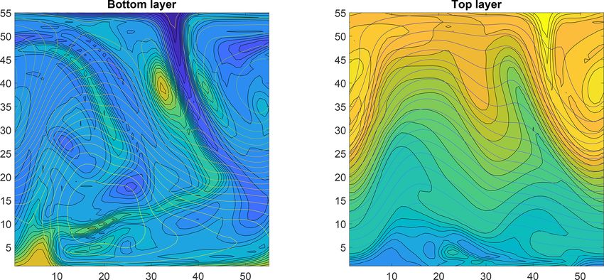
4320                                            S. Springer et al.: Efficient Bayesian inference in chaotic dynamical systems

ference. In fully Bayesian inference, the problem is further        adding “full” likelihood evaluations to the point set used
regularized by prescribing a prior distribution on the model        to construct the local polynomial regression continually im-
state. In practice, Bayesian inference is often realized via        proves the approximation, however. Expensive full likeli-
Markov chain Monte Carlo (MCMC) methods (Gamerman,                  hood evaluations are thus used only to construct the approxi-
1997; Robert and Casella, 2004).                                    mation or “surrogate” model. Conrad et al. (2016) show that,
   This straightforward strategy – for instance, using the          given an appropriate mechanism for triggering likelihood
squared Euclidean distance between model outputs and data           evaluations, the resulting Markov chain converges to the true
to construct a Gaussian likelihood – is, however, inade-            posterior distribution while reducing the number of expen-
quate for chaotic models, where small changes in parame-            sive likelihood evaluations (and hence forward model sim-
ters, or even in the tolerances used for numerical solvers,         ulations) by orders of magnitude. Davis et al. (2020) show
can lead to arbitrarily large differences in model outputs          that
                                                                       √LA-MCMC converges with approximately the expected
(Rougier, 2013). Furthermore, modeling dynamical systems            1/ T error decay rate after a finite number of steps T , and
is often computationally very demanding, which makes sam-           Davis (2018) introduces a numerical parameter that ensures
ple generation time consuming. Since successful application         convergence even if only noisy estimates of the target den-
of MCMC generally requires large numbers of model evalu-            sity are available. This modification is useful for the chaotic
ations, performing Bayesian inference with MCMC is often            systems studied here.
not possible.                                                          The rest of this paper is organized as follows. Section 2
   The present works combines two recent methods to tackle          reviews some additional background literature and related
these problems due to model chaoticity and computational            work and Sect. 3 describes the methodologies used in this
cost. Chaoticity is tamed by using correlation integral likeli-     work, including the CIL, the stochastic LA-MCMC algo-
hood (CIL) (Haario et al., 2015), which is able to constrain        rithm, and the merging of these two approaches. Section 4
the parameters of chaotic dynamical systems. We couple              is dedicated to numerical experiments, where the CIL/LA-
CIL with local approximation MCMC (LA-MCMC) (Conrad                 MCMC approach is applied to several, progressively more
et al., 2016), which is a surrogate modeling technique that         demanding examples. These examples are followed by a con-
makes asymptotically exact posterior characterization fea-          cluding discussion in Sect. 5.
sible for computationally expensive models. We show how
combining these methods enables a Bayesian approach to in-
fer the parameters of chaotic high-dimensional models and           2   Background and related work
quantify their uncertainties in situations previously discussed
                                                                    Traditional parameter estimation methods, which directly
as intractable (Rougier, 2013). Moreover, we introduce sev-
                                                                    utilize the model–observation mismatch, constrain the mod-
eral computational improvements to further enhance the ap-
                                                                    eling to limited time intervals when the model is chaotic.
plicability of the approach.
                                                                    This avoids the eventual divergence (chaotic behavior) of
   The CIL method is based on the concept of fractal di-
                                                                    orbits that are initially close to each other. A classical ex-
mension from mathematical physics, which broadly speaking
                                                                    ample is variational data assimilation for weather prediction,
characterizes the space-filling properties of the trajectory of
                                                                    where the initial states of the model are estimated using ob-
a dynamical system. Earlier work (e.g., Cencini et al., 2010)
                                                                    servational data and algorithms such as 4D-Var, after which
describes a number of different approaches for estimating the
                                                                    a short-time forecast can be simulated (Asch et al., 2016).
fractal dimension. Our previous work extends this concept:
                                                                        Sequential data assimilation methods, such as the Kalman
instead of computing the fractal dimension of a single trajec-
                                                                    filter (KF) (Law et al., 2015), allow parameter estimation
tory, a similar computation measures the distance between
                                                                    by recursively updating both the model state and the model
different model trajectories (Haario et al., 2015), based on
                                                                    parameters by conditioning them on observational data ob-
which a specific summary statistic, called feature vector, is
                                                                    tained over sufficiently short timescales. With methods such
computed. The modification provides a normally distributed
                                                                    as state augmentation, model parameters can be updated as
statistic of the data, which is sensitive to changes in the un-
                                                                    part of the filtering problem (Liu and West, 2001). Alter-
derlying attractor from which the data were sampled. Statis-
                                                                    natively, the state values can be integrated out to obtain the
tics that are sensitive to changes in the attractor yield likeli-
                                                                    marginal likelihood over the model parameters (Durbin and
hood functions that can better constrain the model parame-
                                                                    Koopman, 2012). Hakkarainen et al. (2012) use this filter
ters and therefore also result in more meaningful parameter
                                                                    likelihood approach to estimate parameters of chaotic sys-
posterior distributions.
                                                                    tems. For models with strongly non-linear dynamics, ensem-
   The LA-MCMC method (Conrad et al., 2016, 2018)
                                                                    ble filtering methods provide a useful alternative to the ex-
approximates the computationally expensive log-likelihood
                                                                    tended Kalman filter or variational methods; see Houtekamer
function using local polynomial regression. In this method,
                                                                    and Zhang (2016) for a recent review of various ensemble
the MCMC sampler directly uses the approximation of
                                                                    variants.
the log likelihood to construct proposals and evaluate the
Metropolis acceptance probability. Infrequently but regularly

Geosci. Model Dev., 14, 4319–4333, 2021                                             https://doi.org/10.5194/gmd-14-4319-2021
S. Springer et al.: Efficient Bayesian inference in chaotic dynamical systems                                                   4321

   Filtering-based approaches generally introduce additional      underlying attractor. Due to the nature of the summary statis-
tuning parameters, such as the length of the assimilation         tic used in CIL, the observation time stamps are not explicitly
time window, the model error covariance matrix, and covari-       used. This allows arbitrarily sparse observation time series,
ance inflation parameters. These choices have an impact on        and consecutive observations may be farther than any win-
model parameter estimation and may introduce bias. Indeed,        dow where the system remains predictable. To the best of
as discussed in Hakkarainen et al. (2013), changing the filter-   our knowledge, parameter estimation in this setting has not
ing method requires updating the parameters of the dynam-         been discussed in the literature. Another difference with the
ical model. Alternatives to KF-based parameter estimation         synthetic likelihood approach is that it involves regenerating
methods that do not require ensemble filtering include op-        data for computing the likelihood at every new model param-
erational ensemble prediction systems (EPSs); for example,        eter value, which would be computationally unfeasible in our
ensemble parameter calibration methods by Jarvinen et al.         setting.
(2011) and Laine et al. (2011) have been applied to the In-
tegrated Forecast System (IFS) weather models (Ollinaho
et al., 2012, 2013, 2014) at the European Centre for Medium-      3     Methods
Range Weather Forecasts (ECMWF). However, these ap-
                                                                  3.1    Correlation integral likelihood
proaches are heuristic and again limited to relatively short
predictive windows.                                               We first construct a likelihood function that models the ob-
   Climate model parameters have in previous studies (e.g.,       servations by comparing certain summary statistics of the ob-
Roeckner et al., 2003; ECMWF, 2013; Stevens et al., 2013)         servations to the corresponding statistics of a trajectory sim-
been calibrated by matching summary statistics of quantities      ulated from the chaotic model. As a source of statistics, we
of interest, such as top-of-atmosphere radiation, with the cor-   will choose the correlation integral, which depends on the
responding summary statistics from reanalysis data or out-        fractal dimension of the chaotic attractor. Unlike other statis-
put from competing models. The vast majority of these ap-         tics – such as the ergodic averages of a trajectory – the corre-
proaches produce only point estimates. A fully Bayesian pa-       lation integral is able to constrain the parameters of a chaotic
rameter inversion was performed by Järvinen et al. (2010),        model (Haario et al., 2015).
who inferred closure parameters of a large-scale computa-            Let us denote by
tionally intensive climate model, ECHAM5, using MCMC
and several different summary statistics.                         du
                                                                     = f (u , θ ), u(t = 0) = u0 ,                                (1)
   Computational limitations make applying algorithms such        dt
as MCMC challenging for weather and climate models. Gen-
                                                                  a dynamical system with state u(t) ∈ Rn , initial state u0 ∈
erating even very short MCMC chains may require methods
                                                                  Rn , and parameters θ ∈ Rq . The time-discretized system,
such as parallel sampling and early rejection for tractabil-
                                                                  with time steps ti ∈ {t1 , . . ., tτ } denoting selected observation
ity (Solonen et al., 2012). Moreover, even if these computa-
                                                                  points, can be written as
tional challenges can be overcome, finding statistics that ac-
tually constrain the parameters is difficult, and inference re-   ui ≡ u(ti ) = F (ti ; u0 , θ ).                                 (2)
sults can be thus be inconclusive. The failure of the summary
statistic approach in Järvinen et al. (2010) can be explained     Either the full state ui ∈ Rn or a subset s i ∈ Rd≤n of the state
intuitively: the chosen statistics average out too much infor-    components are observed. We will use S = {s 1 , . . ., s τ } to de-
mation and therefore fail to characterize the geometry of the     note a collection of these observables at successive times.
underlying chaotic attractor in a meaningful way.                    Using the model–observation mismatch at a collection of
   Several Monte Carlo methods have been presented to             times ti to constrain the value of the parameters θ is not
tackle expensive or intractable likelihoods; see, e.g., Luego     suitable when the system (1) has chaotic dynamics, since
et al. (2020) for a recent comprehensive literature review.       the state vector values s i are unpredictable after a finite
Two notable such methods are approximate Bayesian compu-          time interval. Though long-time trajectories s(t) of chaotic
tation (ABC) (Beaumont et al., 2002) and pseudo-marginal          systems are not predictable in the time domain, they do,
sampling (Andrieu and Roberts, 2009). The approach that           however, represent samples from an underlying attractor in
is most closely related to the one presented in this paper is     the phase space. The states are generated deterministically,
Bayesian inference using synthetic likelihoods, which was         but the model’s chaotic nature allows us to interpret the
proposed as an alternative to ABC (Wood, 2010; Price et al.,      states as samples from a particular θ -dependent distribution.
2018). Recent work by Morzfeld et al. (2018) describes an-        Yet obvious choices for summary statistics T that depend
other feature vector approach for data assimilation. For more     on the observed states S, such as ergodic averages, ignore
details and comparisons among these approaches, see the dis-      important aspects of the dynamics and are thus unable to
cussion below in Sect. 3.1.                                       constrain Pthe model parameters. For example, the statistic
   In this work, we employ a different summary statistic,         T (S) = τ1 τi=1 s i is easy to compute and is normally dis-
where the observations are considered as samples from the         tributed in the limit τ → ∞ (under appropriate conditions),

https://doi.org/10.5194/gmd-14-4319-2021                                               Geosci. Model Dev., 14, 4319–4333, 2021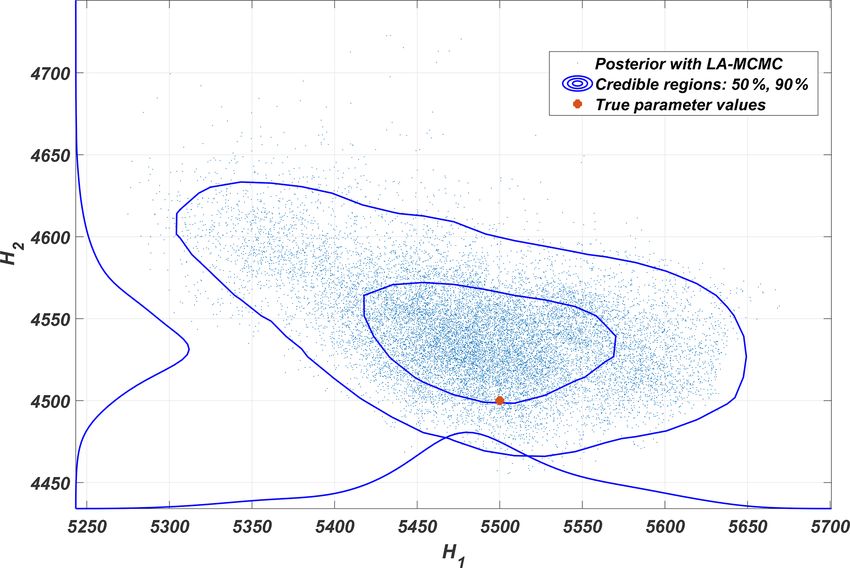
4322                                               S. Springer et al.: Efficient Bayesian inference in chaotic dynamical systems

but this ergodic mean says very little about the shape of the          fines a discretization of the ECDF of the distances k s ki −s lj k,
chaotic attractor.                                                     with discretization boundaries given by the numbers Rm .
                                                                                                k,l
   Instead, we need a summary statistic that retains informa-             Now we define ym          = C(Rm , N, s k , s l ) as components of
tion relevant for parameter estimation but still defines a com-        a statistic T (s , s ) = y k,l := (y0k,l , . . ., yM
                                                                                         k   l                            k,l
                                                                                                                              ). This statistic is
putationally tractable likelihood. To this end, Haario et al.          also called the feature vector. According to Borovkova et al.
(2015) devised the CIL, which retains enough information               (2001) and Neumeyer (2004), the vectors y k,l are normally
about the attractor to constrain the model parameters. We first        distributed, and the estimates of the mean and covariance
                                                                                                √
review the CIL and then discuss how to make evaluation of              converge at the rate nepo to their limit points. This is a gen-
the likelihood tractable.                                              eralization of the classical result of Donsker (1951), which
   We will use the CIL to evaluate the “difference” between            applies to Independent and identically distributed samples
two chaotic attractors. For this purpose, we will first describe       from a scalar-valued distribution. We characterize this nor-
how to statistically characterize the geometry of a given at-          mal distribution by subsampling the full data set S. Specifi-
tractor, given suitable observations S. In particular, construct-      cally, we approximate the mean µ and covariance 6 of T by
ing the CIL likelihood will require three steps: (i) computing         the sample mean and sample covariance of the set {y k,l : 1 ≤
distances between observables sampled from a given attrac-             k, l ≤ nepo , k 6 = l}, evaluated for all 12 nepo (nepo − 1) pairs of
tor; (ii) evaluating the empirical cumulative distribution func-       epochs (s k , s l ) using fixed values of R0 , b, M, and N.
tion (ECDF) of these distances and deriving certain summary               The Gaussian distribution of T effectively characterizes
statistics T from the ECDF; and (iii) estimating the mean and          the geometry of the attractor represented in the data set S.
covariance of T by repeating steps (i) and (ii).                       Now we wish to use this distribution to infer the param-
   Intuitively, the CIL thus interprets observations of a              eters θ . Given a candidate parameter value θ̃ , we use the
chaotic trajectory as samples from a fixed distribution over           model to generate states s ∗(θ̃ ) = {s ∗i (θ̃ )}N   i=1 for the length
phase space. It allows the time between observations to be                                                                                  k,∗
                                                                       of a single epoch. We then evaluate the statistics ym                    =
arbitrarily large – importantly, much longer than the system’s                       k    ∗
                                                                       C(Rm , N, s , s (θ̃ )) as in Eq. (3), by computing the distances
non-chaotic prediction window.                                         between elements of s ∗(θ̃ ) and the states of an epoch s k se-
   Now we describe the CIL construction in detail. Suppose             lected from the data S. Combining these statistics into a fea-
that we have collected a data set S comprising observations of                                       k,∗ M
                                                                       ture vector y k,∗(θ̃ ) = (ym     )m=0 , we can write a noisy esti-
the dynamical system of interest. Let S be split into nepo dif-        mate of the log-likelihood function:
ferent subsets called epochs. The epochs can, in principle, be
any subsets of length N from the reference data set S. In this                           1  k,∗       >
                                                                       log p(θ̃ |s k ) = −  y (θ̃ ) − µ 6 −1 y k,∗(θ̃ ) − µ
paper, however, we restrict the epochs to be time-consecutive                            2
intervals of N evenly spaced observations. Let s k = {s ki }N    i=1                 + constant.                                              (4)
and sl = {s lj }N
                j =1 , with 1 ≤ k, l ≤ nepo and k 6 = l, be two such
disjoint epochs. The individual observable vectors s ki ∈ Rd           Comparing s ∗(θ̃ ) with other epochs drawn from the data set
and s lj ∈ Rd comprising each epoch come from time in-                 S, however, will produce different realizations of the feature
tervals [tkN+1 , t(k+1)N ] and [tlN +1 , t(l+1)N ], respectively. In   vector. We thus average the resulting log likelihoods over all
other words, superscripts refer to different epochs and sub-           epochs:
scripts refer to the time points within those epochs. Haario                               nepo
et al. (2015) then define the modified correlation integral sum                          1 X
                                                                       log p(θ̃ |S) =                log p(θ̃|s k ).                          (5)
C(R, N, s k , s l ) by counting all pairs of observations that are                      nepo   k=1
less than a distance R > 0 from each other:
                                                                       This averaging, which involves evaluating Eq. (4) nepo times,
                      1 X                                            involves only new distance computations and is thus rel-
C(R, N, s k , s l ) = 2       1[0,R] s ki − s lj ,              (3)    atively cheap relative to time integration of the dynamical
                     N i,j ≤N
                                                                       model.
                                                                          Because the feature vectors y k,∗ are random for any fi-
where 1 denotes the indicator function and k · k is the Eu-            nite N, and because the number of epochs nepo is also fi-
clidean norm on Rd . In the physics literature, evaluating             nite, the log likelihood in Eq. (5) is necessarily random. It is
Eq. (3) in the limit R → 0, with k = l and i 6 = j , numerically       then useful to view Eq. (5) as estimate of an underlying true
approximates the fractal dimension of the attractor that pro-          log likelihood. We are therefore in a setting where cannot
duced s k = s l (Grassberger and Procaccia, 1983a, b). Here,           evaluate the unnormalized posterior density exactly; we only
we instead use Eq. (3) to characterize the distribution of dis-        have access to a noisy approximation of it. Previous work
tances between s k and s l at all relevant scales. We assume           (Springer et al., 2019) has demonstrated that derivative-free
that the state space is bounded; therefore, an R0 covering all         optimizers such as the differential evolution (DE) algorithm
pairwise distances in Eq. (3) exists. For a prescribed set of          can successfully identify the posterior mode in this setting,
radii Rm = R0 b−m , with b > 1 and m = 0, . . ., M, Eq. (3) de-        yielding a point estimate of θ. In the fully Bayesian setting,

Geosci. Model Dev., 14, 4319–4333, 2021                                                   https://doi.org/10.5194/gmd-14-4319-2021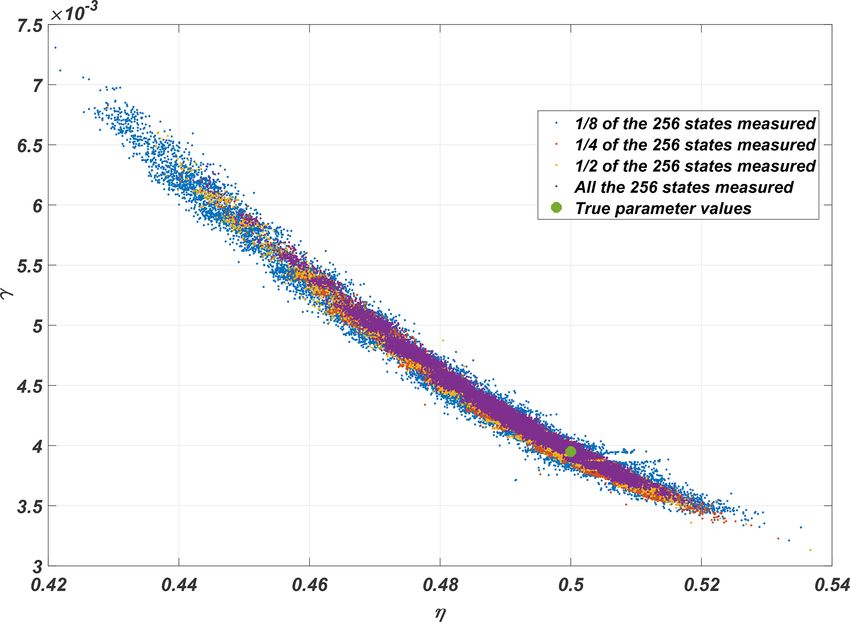
S. Springer et al.: Efficient Bayesian inference in chaotic dynamical systems                                                  4323

one could characterize the posterior p(θ |S) using pseudo-           neously sampling the posterior. The surrogate is incremen-
marginal MCMC methods (Andrieu and Roberts, 2009) but                tally and infinitely refined during sampling and thus tailored
at significant computational expense. Below, we will use a           to the problem – i.e., made more accurate in regions of high
surrogate model constructed adaptively during MCMC sam-              posterior probability. Specifically, the surrogate model is a
pling to reduce this computational burden.                           local polynomial computed by fitting nearby evaluations of
   Note that the CIL approach described above already re-            the “true” log likelihood. We emphasize that the approxi-
duces the computational cost of inference by only requiring          mation itself is not locally supported. At each point θ̃ , we
simulation of the (potentially expensive) chaotic model for          locally construct a polynomial approximation, which glob-
a single epoch. We compare each epoch of the data to the             ally defines a piecewise polynomial surrogate model. This is
same single-epoch model output. Each of these comparisons            an important distinction because the piecewise polynomial
results in an estimate of the log likelihood, which we then          approximation is not necessarily a probability density func-
average over data epochs. A larger data set S can reduce the         tion. In fact, the surrogate function may not even be inte-
variance of this average, but does not require additional sim-       grable. Despite this challenge, Davis et al. (2020) devise a
ulations of the dynamical model. Also, we do not require any         refinement strategy that ensures convergence and bounds the
knowledge about the initial conditions of the model; we omit         error after a finite number of samples. In particular, Davis
an initial time interval before extracting s ∗(θ̃ ) to ensure that   et al. (2020) shows that the error in the approximate Markov
the observed trajectory is on the chaotic attractor.                 chain computed with the local  √ surrogate model decays at ap-
   Moreover, the initial values are randomized for all simu-         proximately the expected 1/ T rate, where T is the number
lations and sampling is started only after the model has in-         of MCMC steps. Davis (2018) demonstrated that noisy esti-
tegrated beyond the initial, predictable, time window. The           mates of the likelihood are sufficient to construct the surro-
independence of the sampled parameter posteriors from the            gate model and still retain asymptotic convergence. Empiri-
initial values was verified both here and in earlier works by        cal studies (Conrad et al., 2016, 2018; Davis et al., 2020) on
repeated experiments.                                                problems of moderate parameter dimension showed that the
   Our approach is broadly similar to the synthetic likelihood       number of expensive likelihood evaluations per MCMC step
method (e.g., Wood, 2010; Price et al., 2018) but differs in         can be reduced by orders of magnitude, with no discernable
two key respects: (i) we use a novel summary statistic that is       loss of accuracy in posterior expectations.
able to characterize chaotic attractors, and (ii) we only need          Here, we briefly summarize one step of the LA-MCMC
to evaluate the forward model for a single epoch. Compar-            construction and refer to Davis et al. (2020) for details. Each
atively, synthetic likelihoods typically use summary statis-         LA-MCMC step consists of four stages: (i) possibly refine
tics such as auto-covariances at a given lag or regression co-       the local polynomial approximation of the log likelihood,
efficients. These methods also require long-time integration         (ii) propose a new candidate MCMC state, (iii) compute
of the forward model for each candidate parameter value θ ,          the acceptance probability, and (iv) accept or reject the pro-
rather than integration for only one epoch. Morzfeld et al.          posed state. The major distinction between this algorithm and
(2018) also discuss several ways of using feature vectors for        standard Metropolis–Hastings MCMC is that the acceptance
inference in geophysics. A distinction of the present work is        probability in stage (iii) is computed only using the approx-
that we use an ECDF-based summary statistic that is prov-            imation or surrogate model of the log likelihood, at both the
ably Gaussian, and we perform extensive Bayesian analysis            current and proposed states. This introduces an error, rela-
of the parameter posteriors via novel MCMC methods. These            tive to computation of the acceptance probability with exact
methods are described next.                                          likelihood evaluations, but stage (i) of the algorithm is de-
                                                                     signed to control and incrementally reduce this error at the
3.2   Local approximation MCMC                                       appropriate rate.
                                                                        “Refinement” in stage (i) consists of adding a compu-
Even with the developments described above, estimating the           tationally intensive log-likelihood evaluation at some pa-
CIL at each candidate parameter value θ̃ is computation-             rameter value θi , denoted by L(θi ), to the evaluated set
ally intensive. We thus use local approximation MCMC (LA-            {(θi , L(θi ))}K
                                                                                    i=1 . These K pairs are used to construct the lo-
MCMC) (Conrad et al., 2016, 2018; Davis et al., 2020) – a            cal approximation via a kernel-weighted local polynomial re-
surrogate modeling method that replaces many of these CIL            gression (Kohler, 2002). The values {θi }K i=1 are called “sup-
evaluations with an inexpensive approximation. Replacing             port points” in this paper. Details on the regression formula-
expensive density evaluations with a surrogate was first in-         tion are in Davis et al. (2020); Conrad et al. (2016). As the
troduced by Sacks et al. (1989) and Kennedy and O’Hagan              support points cover the regions of high posterior probabil-
(2001). LA-MCMC extends these ideas by continually refin-            ity more densely, the accuracy of the local polynomial sur-
ing the surrogate during sampling, which guarantees conver-          rogate will increase. This error is well understood (Kohler,
gence.                                                               2002; Conn et al., 2009) and, crucially, takes advantage of
   First introduced in Conrad et al. (2016), LA-MCMC builds          smoothness in the underlying true log-likelihood function.
local surrogate models for the log likelihood while simulta-         This smoothness ultimately allows the cardinality of the eval-

https://doi.org/10.5194/gmd-14-4319-2021                                               Geosci. Model Dev., 14, 4319–4333, 2021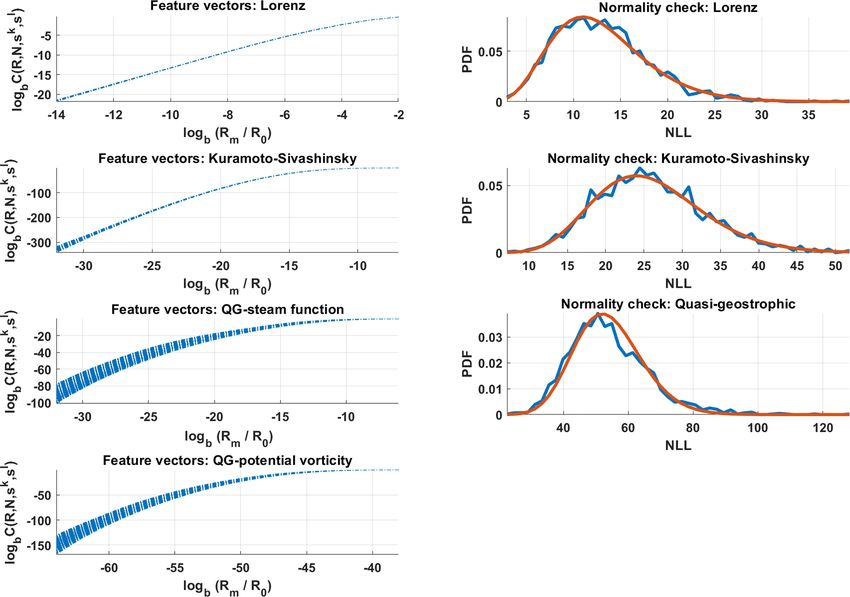
4324                                            S. Springer et al.: Efficient Bayesian inference in chaotic dynamical systems

uated set to be much smaller than the number of MCMC               can be found in the MATLAB implementation available in
steps.                                                             the Supplement.
   Intuitively, if the surrogate converges to the true log like-
lihood, then the samples generated with LA-MCMC will
(asymptotically) be drawn from the true posterior distribu-        4   Numerical experiments
tion. After any finite number of steps, however, the surro-
                                                                   This section contains numerical experiments to illustrate the
gate error introduces a bias into the sampling algorithm. The
                                                                   methods introduced in the previous sections. As a large-scale
refinement strategy must therefore ensure that this bias is
                                                                   example, we characterize the posterior distribution of param-
not the dominant source of error. At the same time, refine-
                                                                   eters in the two-layer quasi-geostrophic (QG) model. The
ments must occur infrequently to ensure that LA-MCMC
                                                                   computations needed to characterize the posterior distribu-
is computationally cheaper than using the true log likeli-
                                                                   tion with standard MCMC methods in this example would
hood. Davis et al. (2020) analyzes the trade-off between
                                                                   be prohibitive without massive computational resources and
surrogate-induced bias and MCMC variance and proposes
                                                                   are therefore omitted. In contrast, we will show that the LA-
a rate-optimal refinement strategy. We use a similar algo-
                                                                   MCMC method is able to simulate from the parameter pos-
rithm, only adding an isotropic `2 penalty on the polyno-
                                                                   terior distribution.
mial coefficients. More specifically, we rescale the variables
                                                                      Before presenting this example, we first demonstrate that
so the max/min values are ±1 – often called coded units –
                                                                   the posteriors produced by LA-MCMC agree with those ob-
then regularize the regression by a penalty parameter (in our
                                                                   tained via exact MCMC sampling methods in cases where
cases, the value α = 1 was found sufficient). This penalty
                                                                   the latter are computationally tractable using two examples:
term modifies the ordinary least squares problem into lo-
                                                                   the classical Lorenz 63 system and the higher-dimensional
cal ridge regression, which improves performance with noisy
                                                                   Kuramoto–Sivashinsky (KS) model. In both examples, we
likelihoods.
                                                                   quantify the computational savings due to LA-MCMC, and
   Our examples use an adaptive proposal density Haario
                                                                   in the second we introduce additional ways to speed up com-
et al. (2006). This choice deviates slightly from the the-
                                                                   putation using parallel (GPU) integration.
ory in Davis et al. (2020), which assumes a constant-in-
                                                                      Let 1t denote the time difference between consecutive ob-
time proposal density. However, this does not necessarily
                                                                   servations; one epoch thus contains the times in the interval
imply that adaptive or gradient-based methods will not con-
                                                                   [iN 1t , (i +1)N 1t ). The number of data points in one epoch
verge. In particular, Conrad et al. (2016) show asymptotic
                                                                   N varies between 1000 and 2000, depending on the example.
convergence using an adaptive proposal density and Con-
                                                                   The training set S consists of a collection of nepo such inter-
rad et al. (2018) strengthen this result by showing that the
                                                                   vals. In all the examples, we choose 1t to be relatively large,
Metropolis-adjusted Langevin algorithm, which is a gradient
                                                                   beyond the predictable window. This is more for demonstra-
based MCMC method, is asymptotically exact when using
                                                                   tion purposes than a necessity; the background theory from
a continually refined local polynomial approximation. These
                                                                   U statistics allows the subsequent state vectors to be weakly
results require some additional assumptions about the target
                                                                   dependent. Numerically, a set of observations that is chosen
density’s tail behavior and the stronger rate optimal result
                                                                   too densely results in the χ 2 test failing, and for this reason
from Davis et al. (2020) has not been shown for such algo-
                                                                   we recommended to always check for normality before start-
rithms. However, in practice, we see that adaptive methods
                                                                   ing the parameter estimation.
still work well in our applications. Exploring the theoretical
                                                                      For numerical tests, one can either use one long time se-
implications of this is interesting and merits further discus-
                                                                   ries or integrate a shorter time interval several times using
sion but is beyond the scope of this paper.
                                                                   different initial values to create the training set for the likeli-
   The parameters of the algorithm are fixed as given in Davis
                                                                   hood. For these experiments, the latter method was used with
et al. (2020), for all the examples discussed here: (i) initial                          n                               k l
                                                                   nepo = 64, yielding epo 2 = 2016 different pairs (s , s ), each
error threshold γ0 = 1; (ii) error threshold decay rate γ1 =
                                                                   of which resulted in an ECDF constructed from N 2 pairwise
1; (iii) maximum poisedness constant 3̄ = 100; (iv) tail-
                                                                   distances. According to tests performed while calibrating the
correction parameter η = 0 (no tail correction); (v) local
                                                                   algorithm, these values of N and nepo are sufficient to ob-
polynomial degree p = 2. The number of nearest neighbors
                                                                   tain robust posterior estimates. With less data, the parameter
k used to construct each local polynomial surrogate is chosen
                                         √                         posteriors will be less precise.
to be k = k0 + (K − k0 )1/3 where k0 = qD, q is the dimen-
                               q                                      The range of the bin radii Rm , m = 0, . . ., M is selected
sion of the parameters θ ∈ R , and D is the number of coeffi-
                                                                   by examining the distances within the training set, keeping
cients in the local polynomial approximation of total degree
                                                                   in mind that a positive variance is needed for every bin to
p = 2, i.e., D = (q + 2)(q + 1)/2. If we had k = D, the ap-
                                                                   avoid a singular covariance matrix. So the largest radius R0
proximation would be an interpolant. Instead, we oversample
             √                                                     can be obtained from
by a factor q, as suggested in Conrad et al. (2016), and al-

low k to grow slowly with the size K of the evaluated set as
in Davis (2018). All these details together with example runs      R0 = min max sik − sjl                                         (6)
                                                                         k6=l   i,j

Geosci. Model Dev., 14, 4319–4333, 2021                                               https://doi.org/10.5194/gmd-14-4319-2021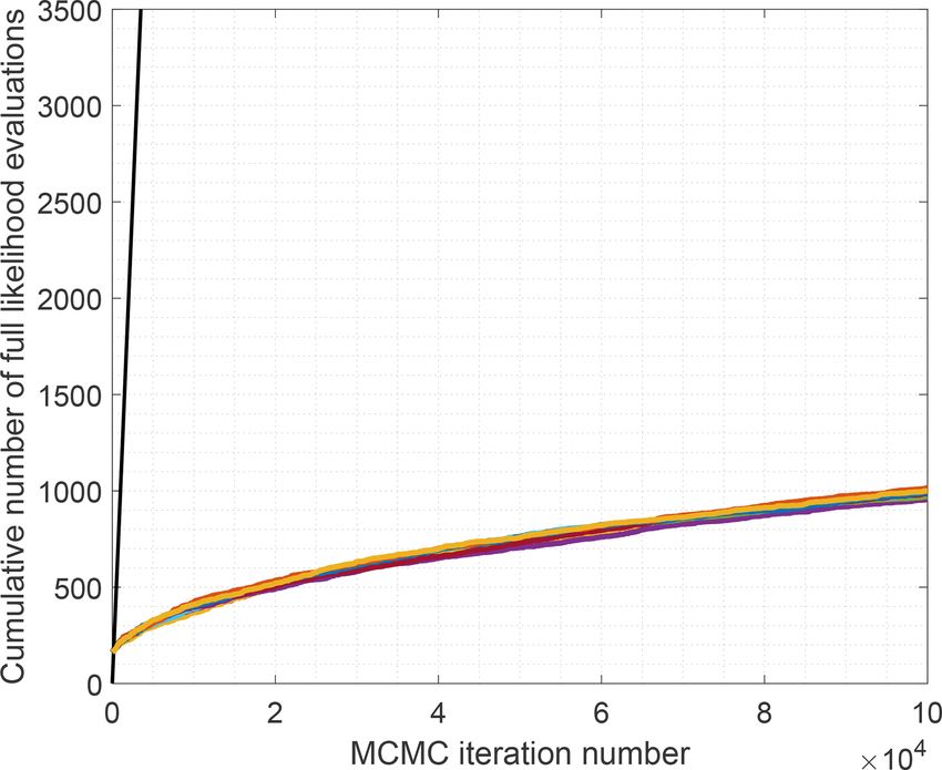
S. Springer et al.: Efficient Bayesian inference in chaotic dynamical systems                                                          4325

over the disjoint subsets of the samples s k and s l of length              4.1   Lorenz 63
N. The smallest radius is selected by requiring that for all the
possible pairs (s k , s l ), it holds that BRM (s ki ) ∩ s l 6 = ∅, where   We use the classical three-dimensional Lorenz 63 system
BRM (s ki ) is the ball of radius RM centered at s ki . That is,            (Lorenz, 1963) as a simple first example to demonstrate
                                                                            how LA-MCMC can be successfully paired with the CIL
                                                                            and the adaptive Metropolis (AM) algorithm (Haario et al.,
                                                                          2001, 2006) to obtain the posterior distribution for chaotic
RM = max min             sik   − sjl       .                         (7)    systems at a greatly reduced computational cost, compared
        k6=l       i,j                                                      to AM without the local approximation. The time evolution
                                                                            of the state vector s = (X, Y, Z) is given by

The base value b is obtained by RM = R0 b−M , and using this                Ẋ = σ (Y − X),
value we fix all the other radii Rm .                                       Ẏ = X(ρ − Z) − Y,
   As always with histograms, the number of bins M must be                  Ż = XY − βZ.                                                (8)
selected first. Too small an M loses information, while too
large values yield noisy histograms, and this noisiness can                 This system of equations is often said to describe an extreme
be seen also in the ECDFs. However, numerical experiments                   simplification of a weather model.
show that the final results – the parameter posteriors – are not               The reference data were generated with parameter values
too sensitive to the specific value of M. For instance, for the             σ = 10, ρ = 28, and β = 83 by performing nepo = 64 distinct
Lorenz 63 case below, the range of M was varied between 5                   model simulations, with observations made at 2000 evenly
and 40, and only a minor decrease of the size of the parameter              distributed times between [10, 20 000]. These observations
posteriors was noticed for increasing M. Any slight increase                were perturbed with 5 % multiplicative Gaussian noise. The
of accuracy comes with a computational cost: higher values                  length of the predictable time window is roughly 7, which
of M increase the stochasticity of the likelihood evaluations,              is less than the time between consecutive observations. The
which leads to smaller acceptance rates in the MCMC sam-                    parameters of the CIL method were obtained as described
pling, e.g., from 0.36 to 0.17 to 0.03 for M = 5, 15, 40, re-               at the start of Sect. 4, with values M = 14, R0 = 2.85, and
spectively, when using the standard adaptive Metropolis sam-                b = 1.51.
pler. In the examples presented in this section, the length M                  The set of vectors {y k,l |k, l ≤ nepo } is shown in Fig. 1 in
of the feature vector is fixed to 14 for the Lorenz 63 model                the log–log scale. The figure shows how the variability of
and 32 for the higher-dimensional KS and QG models.                         these vectors is quite small. Figure 1 validates the normality
   To balance the possibly different magnitudes of the com-                 assumption for feature vectors.
ponents of the state vector, each component is scaled and                      Pairwise two-dimensional marginals of the parameter pos-
shifted to the range [−1, 1] before computing the distances.                terior are shown in Fig. 2, both from sampling the posterior
While this scaling could also be performed in other ways, this              with full forward model simulations (AM) and with using the
method worked well in practice for the models considered.                   surrogate sampling approach for generating the chain. These
The normality of the ensemble of feature vectors is ascer-                  two posteriors are almost perfectly superimposed. Indeed,
tained by comparing the histograms of the quadratic forms                   the difference is at the same level as that between repetitions
in Eq. (4) visually to the appropriate χ 2 distribution.                    of the standard AM sampling alone.
   In all the three experiments, we create MCMC chains                         To get an idea of the computational savings achieved with
of length 105 . However, due to the use of the LA-MCMC                      LA-MCMC, the computation of the MCMC chains of length
approach, the number of full forward model evaluations is                   105 was repeated 10 times. The cumulative number of full
much lower, around 1000 or less; we will report these values                likelihood evaluations is presented in Fig. 3. At the end of
more specifically below.                                                    the chains, the number of full likelihood evaluations varied
   The Lorenz 63 model was integrated with a standard                       between 955 and 1016. Thus, by using LA-MCMC in this
Runge–Kutta solver. The numerical solution of the KS-                       setting, remarkable computational savings of up to 2 orders
model is based on our in-house fast Fourier transform (FFT)-                of magnitude are achieved.
based solver, which runs on the GPU side and is built
around Nvidia compute unified device architecture (CUDA)                    4.2   The Kuramoto–Sivashinsky model
toolchain and cuFFT library (which is a part of the CUDA
ecosystem). The quasi-geostrophic model employs semi-                       The second example is the 256-dimensional Kuramoto–
Lagrangian solver and runs entirely on CPU, but the code has                Sivashinsky (KS) partial differential equation (PDE) system.
been significantly optimized with performance-critical parts,               The purpose of this example is to introduce ways to improve
such as advection operator, compiled using an Intel single                  the computational efficiency by a piecewise parallel integra-
program compiler (ISPC) with support of Advanced Vector                     tion over the time interval of given data. Also, we demon-
Extensions 2 (AVX2) vectorization.                                          strate how decreasing the number of observed components

https://doi.org/10.5194/gmd-14-4319-2021                                                      Geosci. Model Dev., 14, 4319–4333, 2021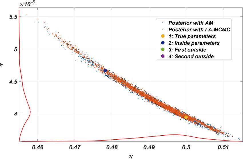
4326                                              S. Springer et al.: Efficient Bayesian inference in chaotic dynamical systems

Figure 1. Left: for all combinations of k and l, the feature vectors for Lorenz 63 and Kuramoto–Sivashinsky, along with concatenated feature
vectors for the quasi-geostrophic system are shown. Right: normality check; the χ 2 density function versus the histograms of the respective
negative log-likelihood (NLL) values; see Eq. (4).

impacts the accuracy of parameter estimation. Even though               (1977) used the same system for describing instabilities of
the posterior evaluation proves to be relatively expensive, di-         laminar flames.
rect verification of the results with those obtained by using             Assume that the solution for this problem can be repre-
standard adaptive MCMC is still possible. The Kuramoto–                 sented by a truncation of the Fourier series
Sivashinsky model is given by the fourth-order PDE:
                                                                                     ∞
                                                                                    X                 2π                    2π
                                                                        s(x, t) =        Aj (t) sin      j x + Bj (t) cos      jx .    (10)
           1                                                                        j =0
                                                                                                       L                     L
st = −ssx − sxx − γ sxxxx ,                                    (9)
           η
                                                                        Using this form reduces Eq. (9) to a system of ordinary dif-
where s = s(x, t) is a real function of x ∈ R and t ∈ R+ . In           ferential equations for the unknown coefficients Aj (t) and
addition, it is assumed that s is spatially periodical with pe-         Bj (t),
riod of L, i.e., s(x + L, t) = s(x, t). This experiment uses the
parametrization from (Yiorgos Smyrlis, 1996) that maps the              Ȧj (t) = α1 j 2 Aj (t) + α2 j 4 Aj (t) + F1 (A(t))            (11)
spatial domain [− L2 , L2 ] to [−π, π ] by setting x̃ = 2π
                                                         L x and
                                                                                        2             4
                                                                        Ḃj (t) = β1 j Bj (t) + β2 j Bj (t) + F2 (B(t)),               (12)
     2
      2π
t˜ = L t. With L = 100, the true value of parameter γ is                where the terms F1 (·) and F2 (·) are polynomials of the vec-
(π/50)2 ≈ 0.0039, and the true value of η becomes 21 . These            tors A and B. For details, see Huttunen et al. (2018). The
two parameters are the ones that are then estimated with the            solution can be effectively computed on graphics processors
LA-MCMC method. This system was derived by Kuramoto                     in parallel, and if computational resources allow, several in-
and Yamada (1976) and Kuramoto (1978) as a model for                    stances of Eq. (9) can be solved in parallel. Even on fast
phase turbulence in reaction–diffusion systems. Sivashinsky             consumer-level laptops, several thousand simulations can be

Geosci. Model Dev., 14, 4319–4333, 2021                                                     https://doi.org/10.5194/gmd-14-4319-2021
S. Springer et al.: Efficient Bayesian inference in chaotic dynamical systems 4327
Figure 2. Two-dimensional posterior marginal distributions of the parameters of the Lorenz 63 model obtained with LA-MCMC and AM.
dow is discarded and 1024 equidistant measurements from
[500, 150 000] are selected, with 1t ≈ 146. The parameters
used for the CIL method were R0 = 1801.7, M = 32, and
b = 1.025.
The time needed to integrate the model up to t = 150 000
is approximately 103 s with the Nvidia 1070 GPU, implying
that generating an MCMC chain with 100 000 samples with
standard MCMC algorithms would take almost 4 months.
The use of LA-MCMC alone again shortens the time needed
by a factor of 100 to around 28 h. However, the calculations
can yet be considerably enhanced by parallel computing. In
practice, this translates the problem of generating a candi-
date trajectory of length 150 000 into generating observations
from several shorter time intervals. In our example, an effi-
cient division is to perform 128 parallel calculations each of
length 4500, with randomized initial values close to the val-
ues selected from the training set. Discarding the predictable
Figure 3. Comparison of the cumulative number of full likelihood interval [0, 500] and taking eight observations at intervals of
evaluations while using AM (black line) and LA-MCMC (colored 500 yields the same number (1024) of observations as in the
lines). Every colored line correspond to a different chain obtained initial setting. While the total integration time increases, this
with LA-MCMC by using the same likelihood. reduces the wall-clock time needed for computation of a sin-
gle candidate simulation from 103 to 2.5 s. The full MCMC
chain can be then be generated in 70 h without the surrogate
performed in parallel when the discretization of the x dimen- model and in 42 min using LA-MCMC.
sion contains around 500 points. Parameter posterior distributions from the KS system, pro-
A total of 64 epochs of the 256-dimensional KS model are duced with MCMC both with and without the local approx-
integrated over the time interval [0, 150 000], and as in the imation surrogate, are shown in Fig. 4. Repeating the cal-
case of the Lorenz 63 model, the initial predictable time win-
https://doi.org/10.5194/gmd-14-4319-2021 Geosci. Model Dev., 14, 4319–4333, 20214328 S. Springer et al.: Efficient Bayesian inference in chaotic dynamical systems
Table 1. Parameter values of the four parameter vectors used in the 4.3 The quasi-geostrophic model
forward KS model simulation examples in Fig. 5. The parameter
vectors in the first column labeled 1 are the true parameters, and The methodology is here applied to a computationally in-
the second one resides inside the posterior. The last two are outside tensive model, where a brute-force parameter posterior es-
the posterior. These parameters correspond to points shown in the timation would be too time consuming. We employ the
posterior distribution shown in Fig. 4. well-known quasi-geostrophic model (Fandry and Leslie,
1984; Pedlosky, 1987) using a dense grid to achieve com-
Case 1 Case 2 Case 3 Case 4 plex chaotic dynamics in high dimensions. The wall-clock
η 0.50000 0.47820 0.49500 0.52000 time for one long-time forward model simulation is roughly
γ 0.00395 0.00467 0.00350 0.00500 10 min, so a naïve calculation of a posterior sample of size
100 000 would take around 2 years. We demonstrate how the
application of the methods verified in the two previous ex-
amples reduces this time to a few hours.
The QG model approximates the behavior on a latitudi-
nal “stripe” at two given atmospheric heights, projected onto
a two-layered cylinder. The model geometry implies peri-
odic boundary conditions, seamlessly stitching together the
extreme eastern and western parts of the rectangular spatial
domain with coordinates x and y. For the northern and south-
ern edges, user-specified time-independent Dirichlet bound-
ary conditions are used. In addition to these conditions and
the topographic constraints, the model parameters include
the mean thicknesses of the two interacting atmospheric lay-
ers, denoted by H1 and H2 . The QG model also accounts for
the Coriolis force. An example of the two-layer geometry is
presented in Fig. 7.
Figure 4. Posterior distribution of the parameters of the KS system. In a non-dimensional form, the QG system can be written
The parameter values are shown in Table 1, while examples of the as
respective integrated trajectories are given in Fig. 5.
q1 = 1ψ1 − F1 (ψ1 − ψ2 ) + βy, (13)
q2 = 1ψ2 − F2 (ψ2 − ψ1 ) + βy + Rs , (14)
culations several times yielded no meaningful differences in
the results. In this experiment, the number of forward model where qi are potential vorticities, and ψi are stream functions
evaluations LA-MCMC needed for generating a chain of with indexes i = 1, 2 for the upper and the lower layers, re-
length 100 000 was in the range [1131, 1221]. spectively. Both the qi and ψi are functions of time t and spa-
Model trajectories from simulations with four different pa- f 2 L2
0
tial coordinates x and y. The coefficients Fi = ǵH control
i
rameter vectors are shown in Fig. 5. These parameter values how much the model layers interact, and β = β0 L/U gives a
were (1) the “true” value which was used to generate training nondimensional version of β0 , the northward gradient of the
data, (2) another parameter from inside the posterior distribu- Coriolis force that gives rise to faster cyclonic flows closer to
tion, and (3–4) two other parameters from outside the poste- the poles. The Coriolis parameter is given by f0 = 2W sin(`),
rior distribution. These parameters are also shown in Fig. 4. where W is the angular speed of Earth and ` is the latitude
Visually inspecting the outputs, cases 1–3 look similar, while of interest. L and U give the length and speed scales, respec-
results using parameter vector 4, furthest away from the pos- tively, and ǵ is a gravity constant. Finally, Rs (x, y) = S(x,y)
ηH2
terior, are markedly different. Even though the third param-
defines the topography for the lower layer, where η = fU0 L
eter vector is outside the posterior, the resulting trajectory is
is the Rossby number of the system. For further details, see
not easily distinguishable from cases 1 and 2, indicating that
Fandry and Leslie (1984) and Pedlosky (1987).
the CIL method differentiates between the trajectories more
It is assumed that the motion determined by the model is
efficiently.
geostrophic, essentially meaning that potential vorticity of
Additional experiments were performed to evaluate the
the flow is preserved on both layers:
stability of the method when not all of the model states were
observed. Keeping the setup otherwise fixed, the number of ∂qi ∂qi ∂qi
elements of the state vectors observed was reduced from the + ui + vi = 0. (15)
∂t ∂x ∂y
full 256 step by step to 128, 64, and 32. The resulting MCMC
chains are presented in Fig. 6, and as expected, when less is Here, ui and vi are velocity fields, which are functions of
observed, the size of the posterior distribution grows. both space and time. They are obtained from the stream func-
Geosci. Model Dev., 14, 4319–4333, 2021 https://doi.org/10.5194/gmd-14-4319-2021S. Springer et al.: Efficient Bayesian inference in chaotic dynamical systems 4329
Figure 5. Example model trajectories from the KS system. Panel (1) shows simulation using the true parameters, the parameters used for
(4) are inside the posterior distribution, and (2) and (3) are generated from simulations with parameters outside the posterior distribution,
shown in Fig. 4. The values of the parameter vectors 1, 2, 3, and 4 are given in Table 1. The y axis shows the 256-dimensional state vector,
and the x axis the time evolution of the system.
Figure 7. An example of the layer structure of the two-layer quasi-
geostrophic model. The terms U1 and U2 denote mean zonal flows,
respectively, in the top and the bottom layer.
Figure 6. Comparison between the KS system’s posterior distribu-
tion in cases where all or only a part of the states are observed.
ities qi are computed according to Eq. (15) for given veloc-
ities ui and vi . With these qi the stream functions can then
tions ψi via be obtained from Eqs. (13) and (14) with a two-stage finite
∂ψi ∂ψi difference scheme.
ui = − , vi = . (16) Finally, the velocity field is updated by Eq. (16) for the
∂y ∂x
next iteration round.
Equations (13)–(16) define the spatiotemporal evolution of For estimating model parameters from synthetic data, a
the quantities qi , ψi , i = 1, 2. reference data set is created with 64 epochs each contain-
The numerical integration of this system is carried out us- ing N = 1000 observations. These data are sampled from the
ing the semi-Lagrangian scheme, where the potential vortic- model trajectory with 1t = 8 (where a time step of length 1
https://doi.org/10.5194/gmd-14-4319-2021 Geosci. Model Dev., 14, 4319–4333, 20214330 S. Springer et al.: Efficient Bayesian inference in chaotic dynamical systems
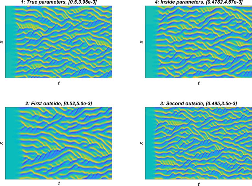
Figure 8. An example of the 6050-dimensional state of the quasi-geostrophic model. The contour lines for both the stream function and
potential vorticity are shown for both layers. Note the cylindrical boundary conditions.
corresponds to 6 h) in the time interval [192, 8192], that In the experiments performed, the number of forward
amounts to a long-range integration of roughly 5–6 years model evaluations needed was ranging in the interval
of a climate model. The spatial domain is discretized into [682, 762], which translates to around 1 week of comput-
a 55 × 55 grid, which results in consistent chaotic behav- ing time. As verified with Kuramoto–Sivashinsky example,
ior and more complex dynamics than with the often-used the forward model integration can be split to segments com-
20 × 40 grid. This is reflected in higher variability in the puted in parallel, which reduced time required to generate
feature vectors, as seen in the Fig. 1. A snapshot of the data for computing the likelihood further with a factor around
6050-dimensional trajectory of the QG system is displayed 50, corresponding to around 3 h for generating the MCMC
in Fig. 8. chain. The pairwise distances for generating the feature vec-
The model state is characterized by two distinct fields, the tors were computed on a GPU, and therefore the required
vorticities and stream functions, that naturally are dependent computation time for doing this was negligible compared to
on each other. As shown in (Haario et al., 2015), it is useful to the model integration time. The posterior distribution of the
construct separate feature vectors to characterize the dynam- two parameters is presented in Fig. 9.
ics in such situations. For this reason, two separate feature
vectors are constructed – one for the potential vorticity on
both layers and the other for the stream function. 5 Conclusions and future work
The Gaussian likelihood of the state is created by stacking
Bayesian parameter estimation with computationally de-
these two feature vectors one after another.
manding computer models is highly non-trivial. The asso-
The normality of the resulting 2(M + 1)-dimensional vec-
ciated computational challenges often become insurmount-
tor may again be verified as shown in Fig. 1. The number of
able when the model dynamics are chaotic. In this work,
bins was set to 32, leading to parameter values R0 = 55 and
we showed it is possible to overcome these challenges by
b = 1.075 for potential vorticity, and R0 = 31, and b = 1.046
combining the CIL with an MCMC method based on lo-
for the stream function.
cal surrogates of the log-likelihood function (LA-MCMC).
For parameter estimation, inferring the layer heights from
The CIL captures changes in the geometry of the underly-
synthetic data is considered. The reference data set with
ing attractor of the chaotic system, while local approxima-
nepo = 64 integrations is produced using the values H1 =
tion MCMC makes generating long MCMC chains based
5500 and H2 = 4500. A single forward model evaluation
on this likelihood tractable, with computational savings of
takes 10 min on a fast laptop, and therefore generating
roughly 2 orders of magnitude, as shown in Table 2. Our
MCMC chains of length 105 with brute force would take
methods were verified by sampling the parameter posteri-
around 2 years to run. As previously, using LA-MCMC again
ors of the Lorenz 63 and the Kuramoto–Sivashinsky mod-
reduces the computation time by a factor of 100.
els, where an (expensive) comparison to exact MCMC with
Geosci. Model Dev., 14, 4319–4333, 2021 https://doi.org/10.5194/gmd-14-4319-2021S. Springer et al.: Efficient Bayesian inference in chaotic dynamical systems 4331
While LA-MCMC has been successfully applied to chains of
dimension up to q = 12 (Conrad et al., 2018), future work
should explore sparsity and other truncations of the local
polynomial approximation to improve scaling with dimen-
sion. From the CIL perspective, calibrating more complex
models, such as weather models, often requires choosing
the part of the state vector from which the feature vectors
are computed. While computing the likelihood from the full
high-dimensional state is computationally feasible, Haario
et al. (2015) showed that carefully choosing a subset of the
state for the feature vectors performs better. Also, the epochs
may need to be chosen sufficiently long to include potential
rare events, so that changes in rare event patterns can be iden-
tified. This, naturally, will increase the computational cost if
Figure 9. The clearly non-Gaussian posterior distribution of the one wants to be confident in the inclusion of such events.
H1 and H2 parameters of the quasi-geostrophic system shows how While answering these questions will require further work,
these parameters anticorrelate with each other. we believe the research presented in this paper provides a
promising and reasonable step towards estimating parame-
Table 2. Summary of results. This table shows the speed-up due ters in the context of expensive operational models.
to the CIL/LA-MCMC combination. Since running the quasi-
geostrophic model 100 000 times was not possible, the nominal
length of the MCMC chain and the speed-up due to LA-MCMC Code availability. The MATLAB code that documents the CIL and
are reported in parentheses in the last column. The numbers of for- LA-MCMC approaches is available in the Supplement. Forward
ward model evaluations with LA-MCMC (second row) are rough model code for performing model simulations (Lorenz, Kuramoto–
averages over several MCMC simulations. Sivashinsky, and quasi-geostrophic model) is also available in the
Supplement.
L63 KS QG
Model evaluations, AM 100 000 100 000 (100 000)
Model evaluations, LA-MCMC 1000 1000 700
Data availability. The data were created using the code provided
Speed-up factor 100 100 (143) in the Supplement.
Supplement. The supplement related to this article is available on-
the CIL was still feasible. Then we applied our approach line at: https://doi.org/10.5194/gmd-14-4319-2021-supplement.
to the quasi-geostrophic model with a deliberately extended
grid size. Without CIL, parameter estimation would not have
been possible with chaotic models such as these; without LA- Author contributions. HH and YM designed the study with input
MCMC, the generation of long MCMC and sufficiently ac- from all authors. SS, HH, AD, and JS combined the CIL and LA-
curate chains for the higher-resolution QG model parame- MCMC methods for carrying out the research. AB wrote and pro-
ters would have been computationally intractable. We note vided implementations of the KS and QG models for GPUs, includ-
that the computational demands of the QG model already get ing custom numerics and testing. SS wrote the CIL code and the
quite close to those of weather models at coarse resolutions. version of LA-MCMC used (based on earlier work by Antti Solo-
We believe that the approach developed here can provide nen), and carried out the simulations. All authors discussed the re-
sults and shared the responsibility of writing the manuscript. SS
ways to solve problems such as the climate model closure
prepared the figures.
parameter estimation investigated in Järvinen et al. (2010)
or long-time assimilation problems with uncertain model pa-
rameters, discussed in Rougier (2013) as unsolved and in-
Competing interests. The authors declare that they have no conflict
tractable. of interest.
There are many potential directions for extension of this
work. First, it should be feasible to run parallel LA-MCMC
chains that share model evaluations in a single evaluated set; Disclaimer. Publisher’s note: Copernicus Publications remains
doing so can accelerate the construction of accurate local neutral with regard to jurisdictional claims in published maps and
surrogate models, as demonstrated in Conrad et al. (2018), institutional affiliations.
and is a useful way of harnessing parallel computational re-
sources within surrogate-based MCMC. Extending this ap-
proach to higher-dimensional parameters is also of interest.
https://doi.org/10.5194/gmd-14-4319-2021 Geosci. Model Dev., 14, 4319–4333, 2021You can also read