Downscaled surface mass balance in Antarctica: impacts of subsurface processes and large-scale atmospheric circulation - The ...
←
→
Page content transcription
If your browser does not render page correctly, please read the page content below
The Cryosphere, 15, 4315–4333, 2021
https://doi.org/10.5194/tc-15-4315-2021
© Author(s) 2021. This work is distributed under
the Creative Commons Attribution 4.0 License.

Downscaled surface mass balance in Antarctica: impacts of
subsurface processes and large-scale atmospheric circulation
Nicolaj Hansen1,2 , Peter L. Langena , Fredrik Boberg1 , Rene Forsberg2 , Sebastian B. Simonsen2 , Peter Thejll1 ,
Baptiste Vandecrux3 , and Ruth Mottram1
1 DMI, Lyngbyvej 100, Copenhagen, 2100, Denmark
2 DTU-Space,   Kongens Lyngby, Denmark
3 Geological Survey of Denmark and Greenland, Copenhagen, Denmark
a now at: iClimate, Department of Environmental Science, Aarhus University, Roskilde, Denmark

Correspondence: Nicolaj Hansen (nichsen@space.dtu.dk)

Received: 24 February 2021 – Discussion started: 17 March 2021
Revised: 9 August 2021 – Accepted: 16 August 2021 – Published: 8 September 2021

Abstract. Antarctic surface mass balance (SMB) is largely        when the SAM is negative. Finally, we compare the mod-
determined by precipitation over the continent and subject to    elled SMB to GRACE data by subtracting the solid ice dis-
regional climate variability related to the Southern Annular     charge, and we find that there is a good agreement in East
Mode (SAM) and other climatic drivers at the large scale.        Antarctica but large disagreements over the Antarctic Penin-
Locally however, firn and snowpack processes are important       sula. There is a large difference between published estimates
in determining SMB and the total mass balance of Antarc-         of discharge that make it challenging to use mass reconcilia-
tica and global sea level. Here, we examine factors that in-     tion in evaluating SMB models on the basin scale.
fluence Antarctic SMB and attempt to reconcile the outcome
with estimates for total mass balance determined from the
GRACE satellites. This is done by having the regional cli-
                                                                 1   Introduction
mate model HIRHAM5 forcing two versions of an offline
subsurface model, to estimate Antarctic ice sheet (AIS) SMB      The Antarctic Ice Sheet (AIS) has the potential to raise global
from 1980 to 2017. The Lagrangian subsurface model esti-         sea level by 58 m (Fretwell et al., 2013) and it is therefore of
mates Antarctic SMB of 2473.5 ± 114.4 Gt yr−1 , while the        utmost importance to understand its role in present sea level
Eulerian subsurface model variant results in slightly higher     change in order to project it into the future. At present the
modelled SMB of 2564.8 ± 113.7 Gt yr−1 . The majority of         AIS contributes 0.3±0.16 mm yr−1 to sea level rise based on
this difference in modelled SMB is due to melt and refreez-      the average ice mass loss of 109 ± 56 Gt yr−1 between 1992
ing over ice shelves and demonstrates the importance of firn     and 2017 (Shepherd et al., 2018). An accelerating mass loss
modelling in areas with substantial melt. Both the Eulerian      has been observed in West Antarctica and over the Antarctic
and the Lagrangian SMB estimates are within uncertainty          Peninsula (AP) in the last 4 decades (Forsberg et al., 2017;
ranges of each other and within the range of other SMB           Rignot et al., 2019). In the light of this acceleration, climatic
studies. However, the Lagrangian version has better statis-      changes are of particular interest due to their role in inducing
tics when modelling the densities. Further, analysis of the      ice sheet dynamic instability, by changing the mass influx to
relationship between SMB in individual drainage basins and       the ice sheet. The ice sheet mass balance (MB) can be split
the SAM is carried out using a bootstrapping approach. This      into atmospheric and ice dynamic components:
shows a robust relationship between SAM and SMB in half
of the basins (13 out of 27). In general, when SAM is positive   MB = SMB − D,                                                (1)
there is a lower SMB over the plateau and a higher SMB on
the westerly side of the Antarctic Peninsula, and vice versa     where D is the solid ice discharge in the form of iceberg calv-
                                                                 ing, and SMB is the surface mass balance composed of pre-

Published by Copernicus Publications on behalf of the European Geosciences Union.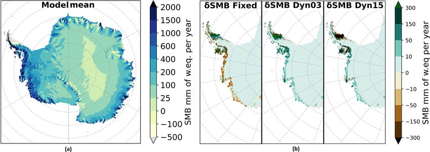
4316                                  N. Hansen et al.: Reconciling different drivers of surface mass balance in Antarctica

cipitation (P , snowfall and rain), sublimation and evapora-       (Mottram et al., 2021), we also compare our modelled SMB
tion (S) from the surface, runoff (RO) of meltwater, and ero-      results with a GRACE gravimetry estimate of the mass bal-
sion of blowing snow. However, blowing snow is not taken           ance to determine any systematic biases. Finally, studies have
into consideration in this study, so the SMB is defined here as    shown that precipitation is not only the largest contributor to
SMB = P −S −RO. Of these components, precipitation is by           Antarctic SMB (Krinner et al., 2007; Agosta et al., 2019),
far the largest contributor (Krinner et al., 2007) and consists    but it also has a spatial heterogeneous distribution vary-
primarily of snow at higher altitudes. Melt and runoff of sur-     ing over time, which affects the SMB (Fyke et al., 2017).
face melt are largely confined to ice shelves and elevations       Regional-scale events like the heavy snowfall in Dronning
less than 1400 m a.m.s.l. (above mean sea level) (Bell et al.,     Maud Land have an important measurable effect on Antarc-
2018). Sublimation and evaporation are however important           tic SMB (Lenaerts et al., 2013; Turner et al., 2019). Differ-
across most of the continent due to low humidity and high          ent representations of these may explain differences between
wind speeds (Palm et al., 2017). If SMB < D, the total mass        modelled SMB (e.g. Mottram et al., 2021) as well as discrep-
balance is negative and the ice sheet loses mass and thereby       ancies between the GRACE mass balance and SMB − D so-
contributes to global sea level rise. Here we focus on the         lutions. Our study therefore also quantifies how regional cli-
SMB component of the mass balance, to pinpoint the imme-           mate indices affect SMB on a basin scale.
diate forcing to ice sheet dynamic instability. To estimate the       Regional circulation patterns including ENSO (El Niño–
SMB, we use an atmospheric regional climate model (RCM)            Southern Oscillation), the BAM (Baroclinic Annular Mode),
to force a subsurface model, which outputs the SMB.                and the Pacific–South American patterns (PSA1 and PSA2)
   Regional climate models are most often used to down-            have previously been identified as important determinants on
scale coarser global models and reanalysis because they            weather and climate variability in Antarctica (Turner, 2004;
add further detail, due to their higher resolution, e.g. in        Irving and Simmonds, 2016; Marshall and Thompson, 2016).
the mountainous areas where the climate can be affected            However, empirical orthogonal functional analysis of South-
by local orography creating katabatic winds or orographic          ern Hemisphere 500 hPa geopotential height (Marshall et al.,
forced precipitation (Rummukainen, 2010; Feser et al., 2011;       2017) demonstrates that the Southern Annular Mode (SAM)
Rummukainen, 2016). Furthermore, RCMs also improve the             is the most important of these regional circulation indices.
physical representations of specific processes over polar ar-      Further, Kim et al. (2020) found a multi-decadal relationship
eas (Lenaerts et al., 2019). Mottram et al. (2021) evaluated       between the SAM and variations in the SMB; for these rea-
Antarctic SMB calculated from the outputs from five differ-        sons we concentrate on its effects in this study. The SAM
ent RCM simulations driven by ERA-Interim (1987–2017).             is an atmospheric phenomenon found across the extratrop-
These five models showed mean annual SMB ranging from              ical Southern Hemisphere that influences the climate over
1961 ± 70 to 2519 ± 118 Gt yr−1 . In the literature, individ-      and around Antarctica (Fogt and Marshall, 2020). Marshall
ual evaluations of different RCMs such as COSMO-CLM2               et al. (2017) found that the phase of the SAM, which de-
(Souverijns et al., 2019), MAR v3.6.4: (Agosta et al., 2019),      scribes pressure anomalies and precipitation in the Southern
and RACMO2.3p2 (van Wessem et al., 2018) are found to              Hemisphere (Fogt and Bromwich, 2006), strongly affects the
be in the same SMB range. The overall model spread in              precipitation pattern over the AIS. Studies have shown that
SMB models corresponds to approximately 2 mm of sea level          the phase of SAM can have a great impact on the surface
change per year. Mottram et al. (2021) also showed that            climate in Antarctica, such as the temperature (Thompson
when compared to in situ observation from both automatic           and Solomon, 2002; Van Lipzig et al., 2008), sea ice ex-
weather stations and glaciological stake measurements, the         tent (Hall and Visbeck, 2002), pressure (Van Den Broeke
data availability proved insufficient to distinguish between       and Van Lipzig, 2004), and especially precipitation (Van Den
better-performing model estimates. Fettweis et al. (2020)          Broeke and Van Lipzig, 2004; Medley and Thomas, 2019).
found similar conclusions for Greenland, where the RCMs            Other studies (Marshall et al., 2017; Dalaiden et al., 2020)
displayed different strengths and weaknesses when evaluated        have found that a positive SAM reduces precipitation over
both spatially and temporally. Mottram et al. (2021) and Ver-      the Antarctic plateau and increases it over the western AP
jans et al. (2021) furthermore showed that subsurface pro-         and in some coastal areas in East Antarctica. Finally Vannit-
cesses that drive melt and refreezing are extremely impor-         sem et al. (2019) found that the Antarctic SMB is influenced
tant when estimating the SMB. Hence, we here include firn          by the SAM in most of the coastal areas of East Antarctica
processes by forcing a newly developed full-subsurface SMB         and large parts of West Antarctica. Therefore, we also in-
model for Antarctica with the RCM HIRHAM5 (Christensen             vestigate the spatial distribution of SMB over the grounded
et al., 2007) over 1979–2017, to assess the effects of firn pro-   AIS (GAIS) in relation to the phase of the SAM.
cesses on estimates of ice sheet SMB. This subsurface model           The aims of this study are thus to estimate present-day
accounts for the physical properties of the uppermost part of      Antarctic SMB using our subsurface model forced with the
the AIS, including density and temperature and the SMB.            RCM HIRHAM5 and compare and evaluate two subsurface
   Acknowledging that it might be challenging to judge the         model versions against each other and in situ data. Further-
performance of the SMB model against in situ observations          more, we estimate the MB, using our modelled SMB re-

The Cryosphere, 15, 4315–4333, 2021                                                   https://doi.org/10.5194/tc-15-4315-2021
N. Hansen et al.: Reconciling different drivers of surface mass balance in Antarctica                                       4317

sults combined with discharge values, and compare it with         Thereby, the subsurface model is forced with the snowfall,
GRACE. Finally, we investigate the relationship between the       rainfall, evaporation, sublimation, and surface energy fluxes
SAM and the SMB. This is done in the following structure:         from HIRHAM5. These include net latent and sensible heat
first, the methods are presented, where the RCM HIRHAM5,          fluxes and downwelling shortwave and longwave radiative
the two subsurface models, and their set-up are described.        fluxes for 6-hourly intervals over the period 1979–2017. To
This is followed by the results, where the modelled SMB           reduce RCM spin-up effects, such as misrepresentation of the
results are shown, including evaluation against in situ mea-      physical state of the atmosphere, e.g. temperature, the first
surements of SMB, firn temperature, and density. Finally, the     year is removed from the results. Furthermore, the model has
MB is estimated and evaluated against GRACE data, and we          been tuned to mimic the average behaviour of the ice sheet
discuss the influence of SAM on SMB, followed by the con-         surface at a 5–12 km scale. It cannot resolve subpixel pro-
clusions.                                                         cesses. However, the small-scale features caused by surface
                                                                  melt translate into an increase in water content in the model.
                                                                  The subsurface scheme is updated hourly by interpolating
2     Methods                                                     the 6-hourly forcing files to 1-hourly time steps. To ensure
                                                                  a smooth transition between two 6-hourly files, a linear in-
2.1    HIRHAM5 regional climate model
                                                                  terpolation in time between the two nearest 6-hourly files is
The HIRHAM5 RCM is a hydrostatic model with 31 atmo-              used. The horizontal resolution of the subsurface model fol-
spheric layers, developed from the physics scheme of the          lows the 0.11◦ native resolution of HIRHAM5.
ECHAM5 global climate model (Roeckner et al., 2003) and              As the Antarctic SMB may be sensitive to the subsurface
the numerical weather forecast model HIRLAM7 (Eerola,             model set-up, here we use two versions of the subsurface
2006). HIRHAM5 has been optimized to model ice sheet              model (Langen et al., 2017). Common for both model ver-
surface processes that are often neglected or simplified in       sions is the albedo scheme, their meltwater percolation, firn
global circulation models. For a full description we refer to     compaction, and heat diffusion schemes. Meltwater in excess
Christensen et al. (2007) and Lucas-Picher et al. (2012). Here    of the irreducible water content (Coléou and Lesaffre, 1998)
HIRHAM5 is forced at the lateral boundaries at 6-hourly in-       is transferred vertically from one layer to the next using a pa-
tervals with relative humidity, temperature, wind vectors, and    rameterization of Darcy flow developed by Hirashima et al.
pressure from the ERA-Interim reanalysis (Dee et al., 2011).      (2010), with hydraulic conductivity values calculated from
Further, daily values for sea ice concentration and sea surface   Van Genuchten (1980) and Calonne et al. (2012) and coeffi-
temperature are also used. HIRHAM5 calculates the full sur-       cients from Hirashima et al. (2010). The impact of ice content
face energy balance at the surface, based on model physics as     on a layer’s conductivity is described by the parameterization
described in Lucas-Picher et al. (2012), Langen et al. (2015)     by Colbeck (1975). When meltwater can infiltrate into a sub-
and Mottram et al. (2017). HIRHAM5 also calculates the            freezing layer, it is refrozen and latent heat is released. Firn
amount of snowfall, rainfall, water vapour deposition and         density is updated at each time step for compaction under
snow sublimation that occurs at the surface. Finally, for the     each layer’s overburden pressure using the parameterization
HIRHAM5 Antarctic simulations, we used the Antarctic do-          by Vionnet et al. (2012).
main defined in the Coordinated Regional Climate Down-               The two model versions differ in the management of the
scaling Experiment (CORDEX) (Christensen et al., 2014)            layers within the model. The first model version developed
and downscaled it further to 0.11◦ (≈ 12.5 km) spatial res-       by Langen et al. (2017) has 32 subsurface layers with a
olution with a dynamical time step of 90 s.                       fixed predefined mass, expressed in metres of water equiva-
                                                                  lent (m w.e.), given by DN = D1 λN−1 , where N is the given
2.2    Subsurface model                                           layer and D1 = 0.065 m w.e. This fixed model implies an Eu-
                                                                  lerian framework, meaning that when snowfall occurs at the
The subsurface model was originally built on ECHAM5               surface, it is added to the first layer, and an equal mass from
physics (Roeckner et al., 2003) but has been updated to           that layer is shifted to the underlying layer. The same goes
include a sophisticated albedo scheme. Following Langen           for each layer in the model column. The same procedure is
et al. (2015) the shortwave albedo is computed internally and     followed when mass is removed from the top layer due to
uses a linear ramping of snow albedo between 0.85 below           runoff or sublimation. Then each layer takes from their un-
−5 ◦ C and 0.65 at 0 ◦ C for the upper-level temperature. The     derlying neighbour an amount of snow/firn equivalent to the
albedo of bare ice is constant at 0.4. Furthermore, a transi-     mass lost at the surface. The temperature and density of the
tion albedo is calculated for thin snow layers on ice, based      layers are updated as the average between the snow or firn
on Oerlemans and Knap (1998) with an e-folding depth of           that is received by the layer, and what remains there. In the
3.2 cm for snow. Moreover, the snow and ice scheme is fur-        following we refer to this model version as the Fixed model.
ther developed and thereby updates the subsurface snow lay-          The second model version uses a Lagrangian frame-
ers with snowfall, melt, retention of liquid water, refreezing,   work for the layer evolution developed by Vandecrux et al.
runoff, sublimation, and rain (Langen et al., 2015, 2017).        (2018, 2020a, b). Layers evolve through a splitting and merg-

https://doi.org/10.5194/tc-15-4315-2021                                                The Cryosphere, 15, 4315–4333, 2021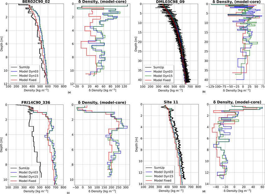
4318                                   N. Hansen et al.: Reconciling different drivers of surface mass balance in Antarctica

ing dynamic based on a number of weighted criteria. This            2.3   Experimental set-up
dynamical model, henceforth referred to as the Dyn model,
has 64 subsurface layers, the number of which are fixed dur-        The Fixed model was initialized with a firn column with uni-
ing the simulation. When snowfall occurs at the surface, it is      form density of 330 kg m−3 and a temperature at the bot-
first stored in a “fresh snow bucket”. When this snow bucket        tom of the firn pack given by the climatological mean of the
reaches 0.065 m w.e., its content is added as a new layer at        HIRHAM5 2 m temperature. Spin-up was performed by re-
the surface of the subsurface scheme, and two layers need to        peating a decade (1980–1989) multiple times. The state of
be merged elsewhere in the model column. The layer merg-            the subsurface at the end of each decade was used as the
ing scheme assesses how likely a layer is to be merged with         initial state for the next iteration. There were no apprecia-
its underlying neighbour based on seven criteria: the layers’       ble shifts in the Antarctic climate from 1980–2019 (Med-
difference in temperature, density, grain size, water content,      ley et al., 2020), so the 1980s can be used as a representa-
ice content, depth, and the thickness of the layers. The first      tive decade for spinning up the subsurface. The Fixed sub-
five criteria make it preferable to merge layers with small         surface scheme was spun up over 25 iterations (250 years).
differences. The sixth criterion makes it preferable to merge       Afterwards, the actual experiment ran from 1979–2017. To
deep layers rather than shallow layers. In this case the shal-      limit computing time, the dynamical model was initialized
low layer limit is set to 5 m w.e.; this criterion carries twice    with the last spin-up from the Fixed model and extrapolated
the weight of the first five. The final criterion says that no      to the 64 layers of the Dyn model. From then, additional
layer can be thicker than a maximum thickness, in this case         spin-ups (1980–1989) ensured that the dynamical splitting
10 m w.e.; this is set to avoid the deepest layers continuing to    and merging of layers had time to evolve throughout the firn
grow. A weighted average of the criteria, where the first five      pack. Two spin-up experiments have been carried out for the
are weighted equally, while the depth and thickness criteria        Dyn model: one that uses 3 decades of additional spin-up
are weighted double and triple respectively, is used by the         (Dyn03), resulting in a total of 280 spin-up years (250 from
model to determine which layers should be merged. When              the fixed model and 30 years in the dynamical model), and
surface sublimation or runoff occurs, it is taken from the          one that uses 15 decades of spin-up (Dyn15), resulting in a
snow bucket and then from the top layer. When a layer de-           total of 400 spin-up years.
creases in thickness and its mass reaches 0.065 m w.e., then           All three model simulations (summarized in Table 1) pro-
it is merged with the underlying layer, and another layer can       vide outputs of monthly and yearly means of all 3D variables
be split in two elsewhere in the model column. The split-           (density, grain size, firn temperature, and ice/water/firn con-
ting routine is based on two criteria: thickness of the layer       tent) and daily 2D fields (SMB, runoff, superimposed ice,
where thick layers are more likely to split and shallowness         melt, albedo, ground heat flux, refreezing, diagnosed snow
where shallow layers are more likely to split. The two cri-         depth (which is an estimate based on the snow concentra-
teria are weighted 60/40. However, the minimum thickness            tion in each layer), and net shortwave and net longwave ra-
of any layer is always 0.065 m w.e. to avoid numerical insta-       diation) of the surface variables. Furthermore daily columns
bility. The bottom of the lowest model layer is assumed to          for specified coordinates interpolated to the nearest grid cell
exchange mass and energy with an infinite layer of ice with         have been retrieved for comparison of in situ measurements.
a temperature, like in the Fixed model (Langen et al., 2015),       For the two simulations with dynamical layer thickness, the
calculated from climatological mean of the HIRHAM5 2 m              daily 3D fields are interpolated into a fixed grid, with the
temperature.                                                        same number of layers, so time averages could be calculated.
    Another difference between the two model versions is that
the dynamic-layer model simultaneously melts the snow and           2.4   Regional drivers and mass balance
ice content of the top layer while the Fixed-layer model melts
the snow content first and then the ice content of the top layer.   The SAM is characterized in Fogt and Bromwich (2006)
This update aims at preventing the top layer from becom-            as the zonal pressure anomalies in the high southern lat-
ing only ice and a barrier to meltwater infiltration. Further-      itudes having opposite sign to those of the midlatitudes.
more, the Dyn model’s runoff is routed downstream using             The SAM drives the westerly winds around Antarctica, but
Darcy’s law and the local surface slope, whereas the Fixed          the stream oscillates north–south. The SAM can have three
model follows Zuo and Oerlemans (1996), and excess water            phases: positive, neutral, or negative, where positive creates
in a layer cannot be transferred to the underlying neighbour.       a higher pressure over the midlatitudes and lower pressure
Both the Fixed and Dyn versions require a fresh snow density        over Antarctica and thus moves the westerly winds closer to
value when adding snowfall at the surface. We here use the          Antarctica. A negative SAM creates a lower pressure over the
Antarctic parameterization from Kaspers et al. (2004), who          midlatitudes and a higher pressure over Antarctica, moving
use local climatological means of skin temperature, 10 m            the westerly winds north. When neutral there is no pressure
wind speed, and accumulation rates; here the means from             difference anomaly. To investigate how the phase of SAM
HIRHAM5 have been used.                                             affects the SMB, monthly SAM data, as calculated by Mar-
                                                                    shall (2018), have been used. From 1980–2017, 261 months

The Cryosphere, 15, 4315–4333, 2021                                                    https://doi.org/10.5194/tc-15-4315-2021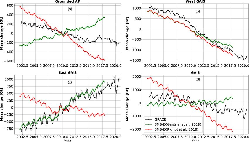
N. Hansen et al.: Reconciling different drivers of surface mass balance in Antarctica                                        4319

Table 1. Model overview and main differences.

                             Fixed                          Dyn03                         Dyn15
             Thickness       Constant over time and space   Varies over time and space    Varies over time and space
             No. of layers   32                             64                            64
             Spin-up [yr]    250                            280                           400
             Melt            First snow and then ice        Snow and ice simultaneously   Snow and ice simultaneously

Figure 1. Mean SMB from 1980 to 2017 in mm yr−1 of w.e. (a) The mean of the model mean; note the nonlinear colour bar. (b) West AIS
where the δSMB has the largest differences between model versions (model minus ensemble mean).

showed a positive SAM (SAM+), 193 months showed a neg-              MB should be equal to SMB minus discharge (SMB − D).
ative SAM (SAM−), and 2 months were neutral. The SAM                So to evaluate our SMB model performance, GRACE and
data are given as one monthly number, i.e. one number for           SMB − D have been plotted. The discharge values were de-
the entire Antarctic domain. To see whether there is a link         rived from two studies: Gardner et al. (2018) and Rignot
between SAM and SMB, the monthly SMB values were di-                et al. (2019). Gardner et al. (2018) gave values from 2008
vided into two groups: SAM+ and SAM−. Then the mean                 and 2015; here we took the mean value and used DGardner
SMB for all months with SAM+ was subtracted from the                over the period. Rignot et al. (2019) have derived decadal
mean SMB for the entire period and likewise for SAM−. To            mean discharge values from 1999–2010 and 2010–2017; for
examine whether there was a statistically robust difference         DRignot the relevant discharge values were used. The SMB
in the δSMB signals, we performed a bootstrapping analy-            value used here is for the grounded AIS only, and since the
sis, using 1200 random resamplings without replacement of           modelled SMB values are quite similar over the grounded
the SAM data, to see whether the δSMB signals could be              AIS, it is only shown here for the Dyn15 simulation.
replicated randomly and if it could be produced randomly
whether the signal would not be robust. Statistically robust-
ness has been defined as δSMB values falling outside the            3   Results
5th–95th percentile range. In order to maintain the seasonal
variability in the SMB, the SAM data were shuffled in sets          In the model mean (1980–2017) of the three SMB sim-
of 12 – in this way the order of the months was maintained          ulations (Fig. 1a), we see that the majority of the total
and thus the seasonal cycle retained. Then confidence inter-        AIS (ToAIS) has a positive SMB; only a few regions show
vals were determined as the 5th and 95th percentiles of the         a negative SMB: Larsen ice shelf, George IV ice shelf,
distribution of the resampled δSMB values.                          coastal regions of Queen Maud Land, the Transantarctic
   Observing the mass balance can be helpful to assess the          Mountains, near Amery ice shelf, and some coastal areas in
spatial patterns of SMB and evaluate the modelled results.          East Antarctica. Near Vostok in East Antarctica, the SMB
Mass balance can be derived from gravimetric measurements           is less than 25 mm w.e. yr−1 . The SMB increases towards
from space. Here GRACE/GRACE-FO mass loss time se-                  the coast due to higher precipitation. The highest SMB is
ries data were computed for the period 2002–2020, using a           greater than 2000 mm w.e. yr−1 and is found on the wind-
mascon approach based on CSR R6 level-2 data, complete              ward (western) side of the AP, whereas the most negative
to harmonic degree 96 (Forsberg et al., 2017). The lowest-          SMB, −500 mm w.e. yr−1 , is found on the leeward (eastern)
degree terms were substituted with satellite laser ranging data     side of the AP (Fig. 1a). All the model simulations show
and glacial isostatic adjustment corrections from the model         nearly identical SMB values over the GAIS; however they
of Whitehouse et al. (2012). From Eq. (1) we know that              differ the most near the coast in West Antarctica and the
                                                                    AP as Fig. 1b shows. Here, we see that δSMB (model mi-

https://doi.org/10.5194/tc-15-4315-2021                                                   The Cryosphere, 15, 4315–4333, 2021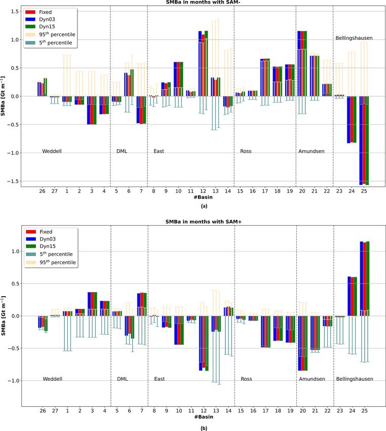
4320 N. Hansen et al.: Reconciling different drivers of surface mass balance in Antarctica
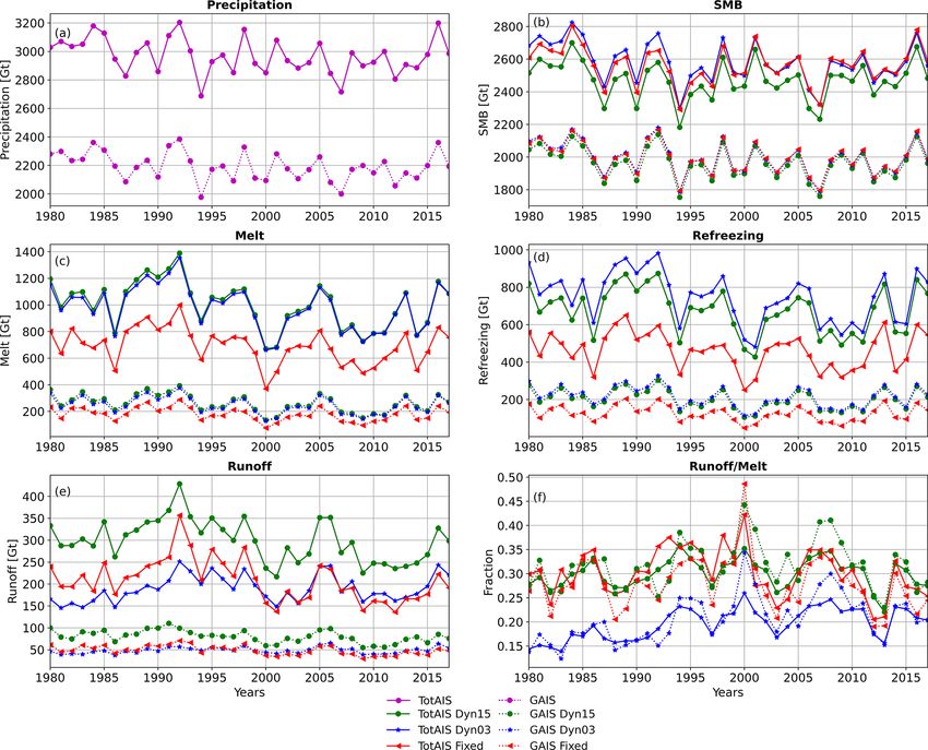
Figure 2. Integrated precipitation (a), SMB (b), melt (c), refreezing (d), and runoff (e) all in Gt yr−1 . Panel (f) shows the runoff to melt
fraction. For the three model simulations, for the entire AIS with ice shelves (ToAIS), and for the GAIS. Note different values on the y axis.
nus mean) shows that the Fixed version has a higher SMB of the SMB, the variability of the modelled SMB closely
of up to 550 mm w.e. over the Larsen ice shelf relative to follows the precipitation variability. The spread in modelled
the model mean. In Dyn03 the SMB values differ between mean melt, refreezing, and runoff are respectively 1 %, 11 %,
−350 and 400 mm w.e. from the model mean. This change and 8 % smaller when including the ice shelves compared
occurs over a few grid cells. In Dyn15 the SMB differs up to to only taking the GAIS, whereas the spread in mean SMB
−650 mm w.e. compared to the model mean over the Larsen becomes 3 % greater. To better compare the melt, refreez-
ice shelf. Since the Fixed version is above the model mean, ing, and runoff from the different simulations, the fraction
over the Larsen ice shelf, and Dyn15 is below the model of runoff to melt is shown in Fig. 2f. Dyn03 has the small-
mean, it looks like the rapid change from negative to positive est runoff fraction whereas Dyn15 and Fixed are quite close
δSMB in Dyn03 over Larsen ice shelf is due to lack of spin- to each other. This implies that even though the magnitudes
up. Below the AP, off the coast of Ellsworth Land and Marie between the simulations are quite different, the refreezing ca-
Byrd Land, the Fixed version models a lower (−75 mm w.e.) pacity of the Fixed and Dyn15 versions are near equal, and
SMB than Dyn03 (35 mm w.e.) and Dyn15 (50 mm w.e.) all Dyn03 has the smallest refreezing capacity. Note also that
relative to the model mean. Around Alexander Island in the the melt is 289 and 309 Gt yr−1 higher in Dyn03 and Dyn15
Bellingshausen Sea, both the Fixed and Dyn15 versions have respectively, compared to the Fixed model. Again this is fo-
a lower SMB compared to Dyn03. The differences in spatial cused largely over the ice shelves, especially over the Larsen
distribution show that in areas where melt occurs, the SMB and Amery ice shelves where Dyn03 and Dyn15 have more
is very sensitive to which subsurface scheme is used. bare ice and thus a lower albedo.
The model differences are seen in the integrated values
for precipitation, SMB, melt, refreezing, and runoff, for both 3.1 Evaluation against observations
ToAIS and the GAIS (Fig. 2), and summarized in Table 2. As
all model simulations are forced using the same precipitation
Koenig and Montgomery (2019) have, in the SumUp dataset,
field (Fig. 2a) and since the precipitation is the main driver
collected accumulation rates over Antarctica. Here we eval-
The Cryosphere, 15, 4315–4333, 2021 https://doi.org/10.5194/tc-15-4315-2021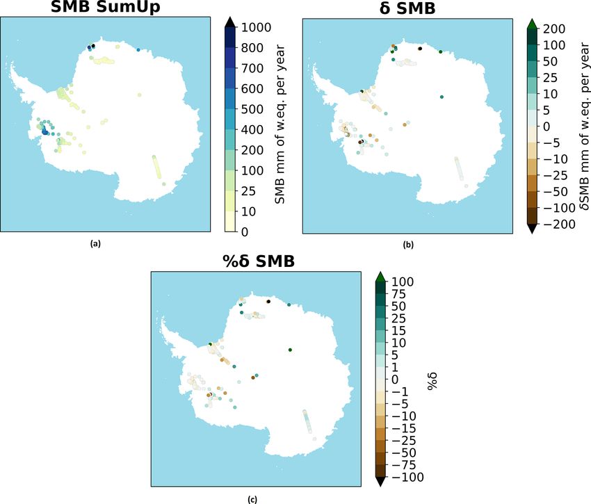
N. Hansen et al.: Reconciling different drivers of surface mass balance in Antarctica                                                   4321

Figure 3. (a) The SMB from SumUp. (b) The δSMB (SumUp minus model ensemble mean) and (c) the change in percent.

Table 2. Yearly mean SMB, melt, refreezing, runoff, precipitation, and runoff fraction (runoff over melt), ± with respective standard devia-
tions, for both the total ice sheet (ToAIS) and the grounded ice sheet (GAIS). Note that all the model simulations are forced with the same
precipitation.

       Model                         SMB                Melt        Refreezing         Runoff         Precipitation   Runoff fraction
                                 [Gt yr−1 ]        [Gt yr−1 ]        [Gt yr−1 ]      [Gt yr−1 ]          [Gt yr−1 ]        [%]
                 ToAIS     2564.8 ± 113.7      695.3 ± 132.4      463.7 ± 97.3    208.3 ± 47.5      2970.9 ± 122.1     0.30 ± 0.06
       Fixed
                 GAIS       1995.2 ± 95.7       180.0 ± 49.5      125.1 ± 40.3     48.8 ± 10.4       2193.8 ± 98.0     0.28 ± 0.05
                 ToAIS     2583.4 ± 121.6      984.2 ± 166.1    748.9 ± 132.5     189.6 ± 29.9                   –     0.20 ± 0.03
       Dyn03
                 GAIS       1995.4 ± 99.3       247.7 ± 61.7     215.3 ± 54.1       48.6 ± 7.0                         0.21 ± 0.05
                 ToAIS     2473.5 ± 114.4     1004.5 ± 173.7    674.5 ± 121.7     299.5 ± 47.1                   –     0.30 ± 0.03
       Dyn15
                 GAIS       1963.3 ± 96.2       262.3 ± 65.8     200.8 ± 51.3      80.6 ± 13.7                         0.32 ± 0.05

uated the modelled SMB values against the SumUp accu-                   than one measurement in one grid cell, an average was used
mulations assuming that over most of the AIS accumulation               (Fig. 3b). Lastly, we computed the change between the ob-
is nearly equivalent to SMB. The SumUp dataset has yearly               servations and the ensemble mean in percent (Fig. 3c). In
measurements for some locations and mean values for longer              total 2221 measurements have been used, located in 251 dif-
periods for other locations. To make it consistent, we com-             ferent grid cells. The SumUp accumulation dataset has areas
puted the yearly mean at each location, shown in Fig. 3a,               with a high concentration of measurements, like Marie Byrd
and compared it with the nearest grid cell in the ensemble              Land, Dronning Maud Land, and Dome Charlie; however, in
mean for the period from 1980 to 2017. If there was more                East Antarctica there are larger areas that are not represented

https://doi.org/10.5194/tc-15-4315-2021                                                           The Cryosphere, 15, 4315–4333, 2021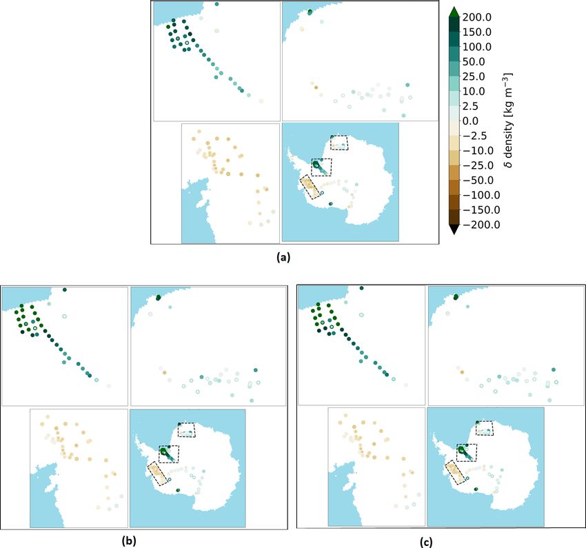
4322 N. Hansen et al.: Reconciling different drivers of surface mass balance in Antarctica
in the SumUp dataset. The accumulation ranges from near
0 to 100 mm w.e. yr−1 at the South Pole, Dronning Maud
Land, and Dome Charlie and up towards 1000 mm w.e. yr−1
in Marie Byrd Land and the coast of Dronning Maud Land.
Figure 3b shows the difference between the model ensemble
mean and the in situ observations where it is seen that there
are some large numerical differences in Marie Byrd Land
and near the coast in Dronning Maud Land. Figure 3c dis-
plays the difference in percent for the δSMB; it shows that
only three of the 251 grid cell comparisons have a difference
greater than ±100 %. Furthermore half of the 251 compari-
son points fit within ±13 %.
Modelled firn densities are evaluated using the SumUp
dataset (Koenig and Montgomery, 2019). When disregarding
firn cores shallower than 2 m, there were 139 density profiles
left (Fig. 4). All the references for the firn profiles can be
found in the reference list. These profiles vary in depth, from
a few metres to 100 m, but the majority are drilled to 10 m
depth. Knowing the coring date, we compare it to the mod-
elled density of the nearest grid cell on the same date. Before
the inter-comparison, the modelled and observed density pro-
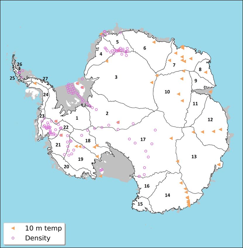
files were interpolated to the same vertical resolution (if the Figure 4. The white colour shows the GAIS, and the grey colours
model resolution is higher than the core resolution, the model show the locations of ice shelves. The spatial distribution of obser-
is interpolated to fit the core resolution and vice versa). In vations are shown with light brown triangles for borehole temper-
the SumUp dataset 96 profiles had the exact date given, and atures and magenta circles for the location of the density profiles.
seven SumUp profiles only had year and month given. Here The grounded basins are derived from Zwally et al. (2012) and out-
the modelled mean density of the given month was com- lined by black lines.
pared. Finally 36 cores had only the year given; in these
cases the modelled mean density of January was compared, Table 3. Mean difference between the modelled and observed firn
as we assume they were most likely collected in the middle of densities (model – core) and standard deviation of the modelled den-
the standard Antarctic summer field season. To evaluate the sities above and below 550 kg m−3 . In total 139 cores were used;
see Fig. 4 for locations.
model performance we calculate mean difference (MD) and
standard deviation (SD) between the modelled and observed
Fixed Dyn03 Dyn15
firn densities. A statistical comparison of the mean differ-
[kg m−3 ] [kg m−3 ] [kg m−3 ]
ence and 1 standard deviation between the firn cores and the
modelled densities is given in Table 3 for the three simula- MD (ρ < 550 kg m−3 ) 43.4 65.6 65.7
tions. Summed up over the AIS, all simulations overestimate SD (ρ < 550 kg m−3 ) 24.2 28.1 26.6
the densities below 550 kg m−3 and underestimate the densi- MD (ρ > 550 kg m−3 ) −19.2 −5.4 −4.1
ties above 550 kg m−3 . It is seen that the Fixed version out- SD (ρ > 550 kg m−3 ) 17.5 21.9 19.4
performs Dyn03 and Dyn15 for densities below 550 kg m−3 .
Conversely, Dyn03 and Dyn15 outperform the Fixed version
for densities above 550 kg m−3 . All three simulations show the mean deviation for densities below 550 kg m−3 would
the best statistics for higher densities. The agreement with be between 36–38 kg m−3 ; for densities above 550 kg m−3
the in situ cores also varies spatially (Fig. 5). Generally the the mean deviation would not change much. Mottram et al.
spatial density bias is consistent between the models. (2021) show that the HIRHAM5 model estimates higher
Over the Filchner–Ronne ice shelf, in Dronning Maud precipitation over the Filchner–Ronne ice shelf than other
Land and in Marie Byrd Land the distribution of profiles RCMs, and the overestimate in density may therefore relate
are quite dense; these areas are marked with boxes (Fig. 5). to overestimated precipitation in this area, which is compli-
All simulations overestimate the density of firn over the ant with our Fig. 3. However, as they also note, the lack of
Filchner–Ronne ice shelf. Of the 36 cores on the Filchner– continuous SMB observations makes it difficult to be certain
Ronne ice shelf, only two have underestimated densities in if and by how much precipitation is overestimated in this re-
the simulations. The rest of the cores have overestimated gion. It could also be due to an overestimation for melt and
densities from 2.5 and up to 200 kg m−3 . In general all three refreezing over the ice shelf.
simulations have the largest biases in this region. If the cores
on the Filchner–Ronne were not included in the statistics,
The Cryosphere, 15, 4315–4333, 2021 https://doi.org/10.5194/tc-15-4315-2021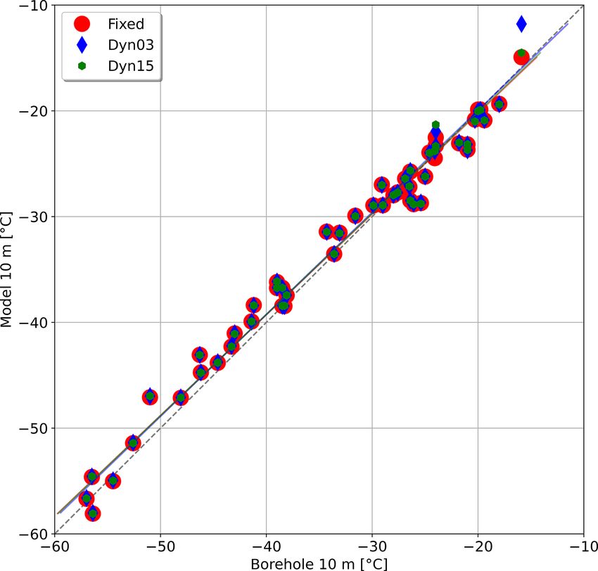
N. Hansen et al.: Reconciling different drivers of surface mass balance in Antarctica                                                   4323

Figure 5. The density bias between simulations and the observations (model minus core). The outer ring represents densities less than
550 kg m−3 , and the inner circle represents densities greater than 550 kg m−3 . Panel (a) is the Fixed model, (b) is Dyn03, and (c) is Dyn15.
Each panel shows the entire AIS with three dashed black boxes. Each box outlines a zoom-in area: from east to west the Dronning Maud
Land, Filchner–Ronne ice shelf, and Marie Byrd Land. All panels have the same colour bar.

   In Dronning Maud Land there are 30 cores with a very                  greater than 550 kg m−3 , with a mean deviation between 10
small bias. The majority of the core densities agree within              and 25 kg m−3 .
±25 kg m−3 , apart from three cores near the coast that are                 For the Ross ice shelf cores and near the South Pole,
overestimated by 100 kg m−3 in all three simulations.                    the Fixed simulation overestimates most of the cores,
   Marie Byrd Land shows a general pattern of underes-                   some of them by 50 to 100 kg m−3 for densities less than
timated densities in 37 cores in all simulations. However,               550 kg m−3 and more than 100 kg m−3 for densities greater
Dyn03 and Dyn15 have lower biases compared to the Fixed.                 than 550 kg m−3 . However, for Dyn03 and Dyn15 we also
In Dyn03 and Dyn15, four cores were underestimated by                    observe an overestimation of most cores, but only six of them
more than 25 kg m−3 , compared to five cores in the Fixed                are overestimated by more than 25 kg m−3 .
model. Both Dyn03 and Dyn15 have six cores where the                        Figure 6 shows 4 of the 139 firn cores: core BER02C90_02
mean deviations are between 0 and 2.5 kg m−3 for densi-                  (Wagenbach et al., 1994) (Fig. 6a), core DML03C98_09
ties less than 550 kg m−3 , but they underestimate densities             (Oerter et al., 2000) (Fig. 6b), core FRI14C90_336 (Graf

https://doi.org/10.5194/tc-15-4315-2021                                                          The Cryosphere, 15, 4315–4333, 2021
4324                                     N. Hansen et al.: Reconciling different drivers of surface mass balance in Antarctica

Figure 6. Examples of density profiles. In each of the four subfigures, the left-hand plot shows the firn core in black and the modelled density
from Fixed, Dyn03, and Dyn15 in red, blue, and green. The right-hand plot shows the difference. The cores are (a) BER02C90_02 taken in
1990 (Wagenbach et al., 1994), (b) DML03C98_09 taken in 1998 (Oerter et al., 2000), (c) FRI14C90_336 taken in 1990 (Graf and Oerter,
2006), and (d) Site 11 taken in 2013 (Morris et al., 2017).

and Oerter, 2006) (Fig. 6c), and core Site 11 (Morris                     We evaluated the model performance using the root-mean-
et al., 2017) (Fig. 6d). These four cores are selected be-                square difference (RMSD), mean difference (MD), and co-
cause they are located in different regions of the AIS,                   efficient of determination (R 2 ). Subsurface temperatures are
and, furthermore, they show different examples of under-                  only sparsely available in Antarctica. The measured 10 m firn
/overestimations of modelled densities. The Fixed simulation              temperatures are compared with the modelled mean 10 m firn
fit quite well (±20 kg m−3 ) with the core taken on Berkner               temperature of the nearest grid cell (Fig. 7). The red, blue,
Island (Fig. 6a), whereas Dyn03 and Dyn15 show a larger                   and green lines are the regression lines of first order, for
bias mainly at the surface and the top 3 m of the firnpack.               Fixed, Dyn03, and Dyn15; they have an R 2 of 0.98, 0.97,
The core from Dronning Maud Land (Fig. 6b) has a high                     and 0.98, respectively. It is assumed that the in situ temper-
vertical resolution; the deeper the cores go, the smaller the             atures are true, so the errors are in the modelled tempera-
biases become. Cores FRI14C90_336 and Site 11 are taken                   tures. For temperatures below −30 ◦ C the three simulations
on the Ronne ice shelf and in Marie Byrd Land respectively.               are in agreement, but in warmer firn temperatures > −30 ◦ C,
The model densities in FRI14C90_336 are overestimated be-                 the agreement becomes worse. The mean deviation of the
low 1 m depth, and the mean bias is 200 kg m−3 . At Site 11               three model simulations is listed Table 4.
all simulations underestimate the density; however below 2 m
depth, the underestimation is nearly constant with a mean
bias of −20 kg m−3 .                                                      4    Discussion
    The modelled subsurface temperatures are evaluated
against observed 10 m firn temperature measurements from                  The annual SMB for the three simulations (Table 2) is of the
49 boreholes (van den Broeke, 2008) (see Fig. 4 for the lo-               same magnitude as the previous HIRHAM5 SMB estimate of
cations). Most of the temperatures were taken in the 1980s                2659 Gt yr−1 for the ToAIS (Mottram et al., 2021). However,
and 1990s; however only the year or decade is known for                   we model a lower SMB, with only Fixed and Dyn03 within 1
when these were taken. Therefore they are compared with                   standard deviation range of Mottram et al. (2021). The lower
the modelled mean 10 m firn temperature from 1980–2000.                   SMB estimates are due to the inclusion of the runoff compo-

The Cryosphere, 15, 4315–4333, 2021                                                             https://doi.org/10.5194/tc-15-4315-2021
N. Hansen et al.: Reconciling different drivers of surface mass balance in Antarctica 4325
Table 4. Mean deviation, root-mean-square deviation, and coeffi- it is 2396 ± 110 Gt (van Wessem et al., 2018). However,
cient of determination, for the modelled and observed 10 m temper- the geographical distribution of precipitation is uneven be-
ature. tween these models, with COSMO-CLM2 being much drier
in western Antarctica than other models in the comparison.
Fixed Dyn03 Dyn15 Even using a common ice mask, Mottram et al. (2021) found
MD [◦ C] 0.42 0.52 0.46 that the difference in precipitation is around 500 Gt yr−1 be-
RMSD [◦ C] 1.66 1.77 1.71 tween HIRHAM5 (the wettest model) and COSMO-CLM2
R2 0.98 0.97 0.98 (the driest model in the intercomparison). The high precipi-
tation in regions of high relief in HIRHAM5 is attributed to a
wet bias in the precipitation scheme, also identified in south-
ern Greenland and similarly occurring in the RACMO2.3p2
regional climate model (Hermann et al., 2018). In both mod-
els this wet bias in steep topography is related to the pre-
cipitation and cloud micro-physics schemes (Mottram et al.,
2021). Areas with a negative SMB can be due to large melt
rates, which is what we see in the model over the Larsen
ice shelf with melt values between 1200 and increasing to-
ward the west to 2300 mm w.e. yr−1 and SMB values in
the range of 300 to 1800 mm w.e. yr−1 increasing toward
the west. In general all three simulations display a higher
melt compared to other RCM studies, e.g. 71 Gt yr−1 in
RACMO2.3p2 (van Wessem et al., 2018) or 40 Gt yr−1 in
MARv3.6.4 (Agosta et al., 2019). These two numbers are
without the AP, but they are nevertheless very low compared
to our melt rates. Trusel et al. (2013) derived satellite-based
melt rate estimates from 1999 to 2009, and over that period,
the Larsen ice shelf experienced the largest melt of around
Figure 7. The dots are 10 m temperature from boreholes vs. mean 400 mm w.e. yr−1 . However, these estimates were derived us-
model 10 m temperature. The solid lines are the regression lines of ing RACMO2.1, and the satellite detects melt areas on the
first order, and the grey dashed line shows the diagonal. Larsen ice shelf that were not simulated in RACMO2.1, most
likely due to coarse resolution, so 400 mm w.e. yr−1 might be
on the low end. Nevertheless, Trusel et al. (2013) estimates
nent in the SMB calculation. The initial SMB results from are still 3 to 6 times lower than our simulation. This suggests
HIRHAM5 in Mottram et al. (2021) were only calculated that the subsurface model may compute a melt rate that is too
from precipitation, evaporation, and sublimation. Calculating high in at least some locations.
the SMB by including a subsurface model results in a more Negative SMB values can also be due to high sublima-
realistic SMB, due to the fact that it takes surface and subsur- tion rates in, e.g., blue ice areas (Hui et al., 2014). For ex-
face processes like energy fluxes, meltwater percolation, and ample, Kingslake et al. (2017) found blue ice in Dronning
refreezing into account. Maud Land and near the Transantarctic Mountains. In these
The spatial distribution of SMB fits reasonably well com- areas our SMB model mean also shows negative SMB be-
pared with the SumUp accumulation measurements; how- tween −50 and −400 mm w.e. yr−1 . A closer investigation
ever, more measurements, especially in East Antarctica, are (not shown) reveals that the negative SMB values in these ar-
needed to be able to do a complete evaluation. Furthermore, eas are driven by the sublimation and thereby consistent with
the spatial distribution of SMB broadly agrees with other the creation of blue ice areas.
studies (Van de Berg et al., 2005; Krinner et al., 2007; Agosta The differences in SMB between the model simulations
et al., 2019; Souverijns et al., 2019). However, the total in- (Fig. 1b) are largest near the coast in West AIS and espe-
tegrated mean SMB in these published studies differs, likely cially on the Larsen ice shelf. This is confirmed in Fig. 2b,
due to a number of different reasons. The ice mask, model where the difference in integrated SMB between the model
resolution and domain, and nudging (if any) are identified simulations is greater when the ice shelves are included. We
as a source of differences in Mottram et al. (2021). How- attribute the differences between the Fixed and Dyn models
ever, differences in model parameterizations affecting com- to the following differences in model designs. The increased
ponents such as sublimation and precipitation are also im- vertical resolution in the Dyn models, with a higher verti-
portant. For example, the modelled annual mean precipita- cal resolution (the top layers can be 6.5 cm w.e. thick) means
tion in HIRHAM5 is 2971 ± 122 Gt, in COSMO-CLM2 it that the cold content in the upper layers is depleted faster,
is 2469 ± 78 (Souverijns et al., 2019), and in RACMO2.3p2 and it starts to melt while the layer below is potentially still
https://doi.org/10.5194/tc-15-4315-2021 The Cryosphere, 15, 4315–4333, 20214326 N. Hansen et al.: Reconciling different drivers of surface mass balance in Antarctica
below freezing. Conversely the top layers in the Fixed model and assessment of the effects of snowpack spin-up in produc-
get thicker rather quickly, which means it takes longer to be ing and using SMB in Antarctica.
brought to melting point and start melting. Furthermore, the Vandecrux et al. (2020b) found that the Fixed version
two versions of the subsurface model have different melting smoothes the firn density profiles, when compared to the
schemes. In both versions one layer can contain snow and dynamical version; this is confirmed by our results. One of
ice at the same time, described with a fraction. However, in the criteria for the dynamical version is that it prefers to
the Fixed model snow melts first and then, if there is more merge layers deeper than 5 m of water equivalent, meaning
energy left, the ice melts. Conversely, the Dyn melts snow that the top 5 m w.e. has a high vertical resolution, which
and ice simultaneously. This simultaneous melting of snow makes it easier to detect changes in density. In areas such as
and ice was introduced in the Dyn version to prevent the the AP, Ronne–Filchner ice shelf, Ross ice shelf, and coastal
top layer from being depleted of its snow content and left areas of Dronning Maud Land where seasonal melt occurs
only with ice (Vandecrux et al., 2018). A top layer composed (Zwally and Fiegles, 1994; Wille et al., 2019), meltwater can
of ice would then prevent surface melt from infiltrating be- percolate into the firn and refreeze, creating ice lenses that
low the top layer. By melting snow and ice simultaneously, change the density but that cannot be detected if the subsur-
there is always snow in the top layer for meltwater infiltra- face scheme has layers with a fixed mass even if the ver-
tion to happen. This difference of infiltration may cause the tical resolution is increased (Vandecrux et al., 2020b). Not
snowmelt to refreeze less and more water to run off than the only is there a difference between the models when evaluat-
simultaneous melt of snow and ice. To investigate these dif- ing density profiles, but this study also shows the importance
ferences in melt, refreezing, and runoff, the runoff fractions of spatial evaluation. Here the three simulations follow the
have been plotted in Fig. 2f and listed in Table 2. Here it is same pattern by over-/underestimating the densities in the
seen that even though the difference in melt between Dyn03 same areas (Fig. 5). This systematic bias may indicate ei-
and Dyn15 is only around 20 Gt yr−1 , the difference between ther further tuning of densification routines is necessary or
the runoff and melt fractions is larger. The Fixed model melts that there are systematic biases in accumulation, leading to
around 300 Gt yr−1 less than the dynamical versions, but the these errors. The subsurface scheme does not currently in-
runoff-to-melt ratio is the same for Fixed and Dyn15. This corporate wind-blowing snow processes that may prove im-
means that Fixed and Dyn15 have the same relative runoff, portant in correcting biases in accumulation. On the other
leading to the same relative refreezing, indicating that this hand, although 0.11◦ is a high-resolution model in Antarctica
difference does not cause a significant partition of melt be- and thus better captures topographic variability than lower-
tween refreezing and runoff. resolution models, it is still relatively coarse when it comes
The difference in SMB between the three simulations to capturing steep topography. Errors in orographic precipita-
confirms how complex it is to estimate the SMB. Just tion are difficult to measure even in well-instrumented basins
by changing the subsurface scheme, the final result dif- and are poorly captured in Antarctica where observations are
fers by 90 Gt yr−1 . By keeping the same subsurface scheme few and far between. The densification bias becomes espe-
and changing the spin-up length, the final result differs by cially important when using altimetry data to estimate the
110 Gt yr−1 . These changes in SMB illustrate the conse- total MB, like in Shepherd et al. (2018) and Rignot et al.
quences of including dynamic firn processes since the layer (2019). Here the firn densification rate is needed to correct
density and temperature and other firn properties are better the altimetry data (Griggs and Bamber, 2011).
conserved, potentially allowing more retention and refreez- Since the density cores are primarily taken from West
ing where there is capacity or reducing it where there is not. Antarctica and Dronning Maud Land, these statistics rep-
Although these differences are currently only a few percent resent complex areas with high precipitation and melt–
of the total SMB, as the climate warms and melt becomes refreezing events, whereas density comparisons from less
more widespread in Antarctica (e.g. Boberg et al., 2020; Kit- complex areas (low precipitation and no melt–refreezing)
tel et al., 2021), accounting for these processes will become such as East Antarctica are sparse. Nonetheless they are still
more important. Moreover, on local and regional scales, the very important. Based on the statistics from these model set-
differences are more important when determining mass bal- ups, the Dyn version is preferred when modelling densities
ance in basins or outlet glacier/ice shelves. above 550 kg m−3 .
The differences between versions with a different spin-up The simulated 10 m firn temperature depends on the thick-
period suggest that the snowpack is not quite in equilibrium ness and number of layers above the 10 m point. The thick-
in all locations. Therefore, SMB calculations consequently ness of a layer determines how conductive heat fluxes are
vary due to the amount of melt calculated during the initial- resolved in the near-surface snow. A thicker layer will have
ization period. Retention and refreezing of meltwater during more thermal inertia and will require more energy to be
spin-up cause different profiles of temperature and density to warmed up. A thin layer can respond much more quickly
develop depending on how long the spin-up lasts. These re- to fluctuations in the surface energy balance. Differences in
sults therefore emphasize the importance of adequate spin-up simulated temperatures between models, as we see in Ta-
ble 4, can therefore be explained by vertical resolution, which
The Cryosphere, 15, 4315–4333, 2021 https://doi.org/10.5194/tc-15-4315-2021N. Hansen et al.: Reconciling different drivers of surface mass balance in Antarctica 4327
Figure 8. Integrated relative mass change over the grounded Antarctic Peninsula (a), the grounded West AIS (b), grounded East AIS (c), and
the GAIS (d). GRACE relative mass change from 2002 to 2020 (black graph). SMB minus discharge (green/red graphs). SMB values are
from the Dyn15 simulation, and discharge values are derived by Gardner et al. (2018) (in green) and Rignot et al. (2019) (in red). Note that
the y axis differs from panel to panel.
affects both their calculation of temperature and how the heat a smaller mass loss in the beginning of the period, and then
is conducted to a depth of 10 m. Note that the models also use around 2009 the GRACE mass loss increases. Both Gardner
different thermal conductivity parameterizations. et al. (2018) and Rignot et al. (2019) have found an increas-
ing discharge in West Antarctica. However due to the limited
4.1 Satellite gravimetric mass balance temporal resolution from Gardner et al. (2018), the discharge
is assumed constant, resulting in an equal offset in SMB − D
from 2002–2009, but then diverging results from 2010. This
Over the AP there is a large disagreement between
shows that in areas where there are large changes in the dy-
SMB − DGardner and SMB − DRignot , the mean discharge
namic mass loss, discharge values with a higher temporal res-
values differ by 90 Gt yr−1 , with DRignot being the largest.
olution are needed.
This results in opposite trends of SMB − D. SMB − DGardner
Over the East GAIS the agreement between GRACE and
shows a mass gain of around 600 Gt, and SMB − DRignot
SMB − DGardner is remarkably good. Between 2009 and
shows approximate mass loss of 1150 Gt over the period,
2011 large snowfall events were observed in Dronning Maud
whereas GRACE has a mass loss of around 400 Gt for the pe-
Land (Boening et al., 2012; Lenaerts et al., 2013) (basins 5–
riod (Fig. 8a). There are times when the variability between
8 in Fig. 4). These snowfall events led to rapid mass gain,
GRACE and the two SMB-D graphs follows each other,
which is seen in both GRACE and SMB − DGardner , espe-
e.g. local peak around year 2006, 2011, and 2017. Since the
cially in 2009–2010 (Fig. 8c). This mass gain is less pro-
discharge is plotted as a constant, this variability originates
nounced in SMB − DRignot because it estimates an overall
from the SMB model, most likely precipitation. This means
mass loss for the period. In the SMB signal there are yearly
that the DGardner value is too small, DRignot values are too
variabilities; however, these variabilities are larger in the
large, or the SMB magnitude is too low or high depending
GRACE data compared to SMB − D. For the entire GAIS
on which discharge is used. As the resolution of GRACE is
GRACE detects a mass loss of 900 Gt, SMB − DGardner
quite coarse, it can add to the uncertainties over the AP, be-
shows a mass gain of 500 Gt, and SMB − DGardner shows
cause of narrow topography. Over the grounded West AIS
a mass loss of 4000 Gt, for the overlapping period 2002–
the trend of GRACE, SMB − DRignot , and SMB − DGardner
2017. The majority of that difference between GRACE and
agrees. They all see a mass loss, of around 2000, 2150, and
SMB − DGardner can be attributed to the AP. The difference
1700 Gt, respectively, for the overlapping period (Fig. 8b).
between GRACE and SMB − DRignot arises from the AP and
The discharge values from the two studies differ only by
East GAIS.
2 Gt yr−1 from 2002 to 2010 but by 50 Gt yr−1 from 2010
to 2017, with DGardner being the lowest. GRACE measures
https://doi.org/10.5194/tc-15-4315-2021 The Cryosphere, 15, 4315–4333, 2021You can also read