Dual-satellite (Sentinel-2 and Landsat 8) remote sensing of supraglacial lakes in Greenland - The Cryosphere
←
→
Page content transcription
If your browser does not render page correctly, please read the page content below
The Cryosphere, 12, 3045–3065, 2018
https://doi.org/10.5194/tc-12-3045-2018
© Author(s) 2018. This work is distributed under
the Creative Commons Attribution 4.0 License.

Dual-satellite (Sentinel-2 and Landsat 8) remote sensing of
supraglacial lakes in Greenland
Andrew G. Williamson1 , Alison F. Banwell1,2 , Ian C. Willis1,2 , and Neil S. Arnold1
1 Scott   Polar Research Institute, University of Cambridge, Cambridge, UK
2 Cooperative    Institute for Research in Environmental Sciences, University of Colorado Boulder, Boulder, Colorado, USA

Correspondence: Andrew G. Williamson (agw41@alumni.cam.ac.uk)

Received: 16 March 2018 – Discussion started: 20 April 2018
Revised: 3 September 2018 – Accepted: 7 September 2018 – Published: 26 September 2018

Abstract. Remote sensing is commonly used to monitor              events and, by analysing downscaled regional climate-model
supraglacial lakes on the Greenland Ice Sheet (GrIS); how-        (RACMO2.3p2) run-off data, the water quantity that enters
ever, most satellite records must trade off higher spatial res-   the GrIS via the moulins opened by such events. We find that
olution for higher temporal resolution (e.g. MODIS) or vice       during the lake-drainage events alone, the water drained by
versa (e.g. Landsat). Here, we overcome this issue by devel-      small lakes (< 0.125 km2 ) is only 5.1 % of the total water
oping and applying a dual-sensor method that can monitor          volume drained by all lakes. However, considering the to-
changes to lake areas and volumes at high spatial resolu-         tal water volume entering the GrIS after lake drainage, the
tion (10–30 m) with a frequent revisit time ( ∼ 3 days). We       moulins opened by small lakes deliver 61.5 % of the total
achieve this by mosaicking imagery from the Landsat 8 Op-         water volume delivered via the moulins opened by large and
erational Land Imager (OLI) with imagery from the recently        small lakes; this is because there are more small lakes, allow-
launched Sentinel-2 Multispectral Instrument (MSI) for a          ing more moulins to open, and because small lakes are found
∼ 12 000 km2 area of West Greenland in the 2016 melt sea-         at lower elevations than large lakes, where run-off is higher.
son. First, we validate a physically based method for calculat-   These findings suggest that small lakes should be included in
ing lake depths with Sentinel-2 by comparing measurements         future remote-sensing and modelling work.
against those derived from the available contemporaneous
Landsat 8 imagery; we find close correspondence between
the two sets of values (R 2 = 0.841; RMSE = 0.555 m). This
provides us with the methodological basis for automati-           1   Introduction
cally calculating lake areas, depths, and volumes from all
available Landsat 8 and Sentinel-2 images. These automatic        In the summer, supraglacial lakes (hereafter “lakes”) form
methods are incorporated into an algorithm for Fully Au-          within the ablation zone of the Greenland Ice Sheet (GrIS),
tomated Supraglacial lake Tracking at Enhanced Resolu-            influencing the GrIS’s accelerating mass loss (van den
tion (FASTER). The FASTER algorithm produces time se-             Broeke et al., 2016) in two main ways. First, because the
ries showing lake evolution during the 2016 melt season, in-      lakes have low albedo, they can directly affect the surface
cluding automated rapid (≤ 4 day) lake-drainage identifica-       mass balance through enhancing ablation relative to the sur-
tion. With the dual Sentinel-2–Landsat 8 record, we iden-         rounding bare ice (Lüthje et al., 2006; Tedesco et al., 2012).
tify 184 rapidly draining lakes, many more than identified        Second, many lakes affect the dynamic component of the
with either imagery collection alone (93 with Sentinel-2;         GrIS’s mass balance when they drain either “slowly” or
66 with Landsat 8), due to their inferior temporal resolu-        “rapidly” in the middle to late melt season (e.g. Palmer et
tion, or would be possible with MODIS, due to its omis-           al., 2011; Joughin et al., 2013; Chu, 2014; Nienow et al.,
sion of small lakes < 0.125 km2 . Finally, we estimate the wa-    2017). Slowly draining lakes typically overtop and incise
ter volumes drained into the GrIS during rapid-lake-drainage      supraglacial streams in days to weeks (Hoffman et al., 2011;
                                                                  Tedesco et al., 2013), while rapidly draining lakes drain by

Published by Copernicus Publications on behalf of the European Geosciences Union.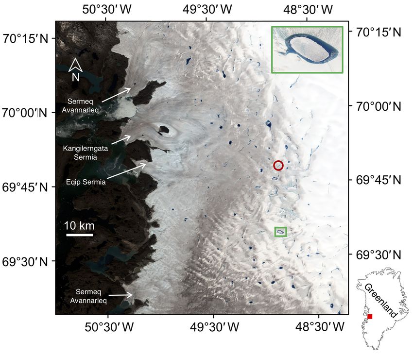
3046                             A. G. Williamson et al.: Dual-satellite remote sensing of supraglacial lakes in Greenland

hydrofracture in hours to days (Das et al., 2008; Doyle et al.,   gest that increased summer velocities may not be offset by
2013; Tedesco et al., 2013; Stevens et al., 2015).                later ice velocity decreases (Doyle et al., 2014; de Fleurian
   Rapid lake drainage plays an important role in the GrIS’s      et al., 2016), and it is unclear whether hydrofracture can
negative mass balance because the large volumes of lake wa-       occur within these regions, due to the thicker ice and lim-
ter can reach the subglacial drainage system, perturbing it       ited crevassing (Dow et al., 2014; Poinar et al., 2015). These
from a steady state, lowering subglacial effective pressure,      unknowns inland add to the uncertainty in predicting future
and enhancing basal sliding over hours to days (Shepherd et       mass loss from the GrIS. There is a need, therefore, to study
al., 2009; Schoof, 2010; Bartholomew et al., 2011a, b, 2012;      the seasonal filling and drainage of lakes on the GrIS, and
Hoffman et al., 2011; Banwell et al., 2013, 2016; Tedesco et      to understand its spatial distribution and inter-annual varia-
al., 2013; Andrews et al., 2014), particularly if the GrIS is     tion, in order to inform the boundary conditions for GrIS hy-
underlain by sediment (Bougamont et al., 2014; Kulessa et         drology and ice-dynamic models (Banwell et al., 2012, 2016;
al., 2017; Doyle et al., 2018; Hofstede et al., 2018). Rapid-     Leeson et al., 2012; Arnold et al., 2014; Koziol et al., 2017).
lake-drainage events also have two longer-term effects. First,       Remote sensing has helped to fulfil this goal (Hock et
they open moulins, either directly within lake basins (Das et     al., 2017; Nienow et al., 2017), although it usually involves
al., 2008; Tedesco et al., 2013) or in the far field if pertur-   trading off either higher spatial resolution for lower tempo-
bations in stress exceed the tensile strength of ice (Hoffman     ral resolution, or vice versa. For example, the Landsat and
et al., 2018), sometimes leading to a cascading lake-drainage     ASTER satellites have been used to monitor lake evolution
process (Christoffersen et al., 2018). These moulins deliver      (Sneed and Hamilton, 2007; McMillan et al., 2007; Geor-
the bulk of surface meltwater to the ice-sheet bed (Koziol et     giou et al., 2009; Arnold et al., 2014; Banwell et al., 2014;
al., 2017), explaining the observations of increased ice veloc-   Legleiter et al., 2014; Moussavi et al., 2016; Pope et al.,
ities over monthly to seasonal timescales within some sectors     2016; Chen et al., 2017; Miles et al., 2017; Gledhill and
of the GrIS (Zwally et al., 2002; Joughin et al., 2008, 2013,     Williamson, 2018; Macdonald et al., 2018). While this work
2016; Bartholomew et al., 2010; Colgan et al., 2011; Hoff-        involves analysing lakes at spatial resolutions of 30 or 15 m,
man et al., 2011; Palmer et al., 2011; Banwell et al., 2013,      the best temporal resolution that can be achieved using these
2016; Cowton et al., 2013; Sole et al., 2013; Tedstone et         satellites is ∼ 4 days and is often much longer due to the
al., 2014; Koziol and Arnold, 2018). Second, the fractures        satellites’ orbital geometry and/or site-specific cloud cover,
generated during drainage allow surface meltwater to reach        which can significantly affect the observational record on the
the subfreezing ice underneath, potentially increasing the ice-   GrIS (Selmes et al., 2011; Williamson et al., 2017). This
deformation rate over longer timescales (Phillips et al., 2010,   presents an issue for identifying rapid lake drainage with
2013; Lüthi et al., 2015), although the magnitude of this ef-     confidence since hydrofracture usually occurs in hours (Das
fect is unclear (Poinar et al., 2017). Alternatively, the water   et al., 2008; Doyle et al., 2013; Tedesco et al., 2013). An al-
might promote enhanced subglacial conduit formation due to        ternative approach involves tracking lakes at high temporal
increased viscous heat dissipation (Mankoff and Tulaczyk,         (sub-daily) resolution but at lower spatial resolution (∼ 250–
2017). Although rapidly and slowly draining lakes are dis-        500 m) using MODIS imagery (Box and Ski, 2007; Sundal
tinct, they can influence each other synoptically if, for ex-     et al., 2009; Selmes et al., 2011, 2013; Liang et al., 2012;
ample, the water within a stream overflowing from a slowly        Johansson and Brown, 2013; Johansson et al., 2013; Mor-
draining lake reaches the ice-sheet bed, thus causing basal       riss et al., 2013; Fitzpatrick et al., 2014; Everett et al., 2016;
uplift or sliding, and thereby increasing the propensity for      Williamson et al., 2017, 2018). However, this lower spatial
rapid lake drainage nearby (Tedesco et al., 2013; Stevens et      resolution means that lakes < 0.125 km2 cannot be confi-
al., 2015).                                                       dently resolved (Fitzpatrick et al., 2014; Williamson et al.,
   While lake drainage is known to affect ice dynamics over       2017) and even lakes that exceed this size are often omitted
short (hourly to weekly) timescales, greater uncertainty sur-     from the satellite record (Leeson et al., 2013; Williamson et
rounds its longer-term (seasonal to decadal) dynamic impacts      al., 2017).
(Nienow et al., 2017). This is because the subglacial drainage       Because of the problems associated with the frequency
system in land-terminating regions may evolve to higher hy-       or spatial resolution of these satellite records, it has been
draulic efficiency, or water may leak into poorly connected       suggested that greater insights into GrIS hydrology might
regions of the bed, producing subsequent ice velocity slow-       be gained if the images from multiple satellites could be
downs either in the late summer, winter, or longer term (van      used simultaneously (Pope et al., 2016). Miles et al. (2017)
de Wal et al., 2008, 2015; Bartholomew et al., 2010; Hoff-        were the first to present such a record of lake observations
man et al., 2011, 2016; Sundal et al., 2011; Sole et al., 2013;   in West Greenland, combining imagery from the Sentinel-1
Tedstone et al., 2015; de Fleurian et al., 2016; Stevens et       Synthetic Aperture Radar (SAR) (hereafter “Sentinel-1”) and
al., 2016). Despite this observed slowdown for some of the        Landsat 8 Operational Land Imager (OLI) (hereafter “Land-
GrIS’s ice-marginal regions, greater uncertainty surrounds        sat 8”) satellites, and developing a method for tracking lakes
the impact of lake drainage on ice dynamics within interior       at high spatial (30 m) and temporal resolution (∼ 3 days).
regions of the ice sheet, since fieldwork and modelling sug-      Using Sentinel-1 imagery facilitated lake detection through

The Cryosphere, 12, 3045–3065, 2018                                                    www.the-cryosphere.net/12/3045/2018/
A. G. Williamson et al.: Dual-satellite remote sensing of supraglacial lakes in Greenland 3047
clouds and in darkness, enabling, for example, lake freeze- volume measurements for each lake in the study region
over in the autumn to be studied. This approach permitted to show their seasonal evolution.
the identification of many more lake-drainage events than
would have been possible if either set of imagery had been 3. We aim to identify lakes that drain rapidly (in ≤ 4 days)
used individually, as well as the drainage of numerous small using the automatic algorithm, separating these lakes
lakes that could not have been identified with MODIS im- into small (< 0.125 km2 ) and large (≥ 0.125 km2 ) cat-
agery (Miles et al., 2017). Monitoring all lakes, including egories, based on whether they could be identified with
the smaller ones, many of which may also drain rapidly by MODIS.
hydrofracture, is important since recent work shows that a
key determinant on subglacial-drainage development is the 4. We aim to quantify the run-off volumes routed into the
density of surface-to-bed moulins opened by hydrofracture, GrIS both during the lake-drainage events themselves
rather than the hydrofracture events themselves (e.g. Banwell and afterwards via moulins opened by hydrofracture, for
et al., 2016; Koziol et al., 2017). However, since Miles et the small and large lakes.
al. (2017) used radar imagery, lake water volumes could not
be calculated, restricting the type of information that could
be obtained. 2 Data and methods
The Sentinel-2 Multispectral Instrument (MSI) com-
Here, we describe the study region (Sect. 2.1), the collec-
prises the Sentinel-2A (launched in 2016) and Sentinel-
tion and pre-processing of the Landsat 8 and Sentinel-2 im-
2B (launched in 2017) satellites, which have 290 km swath
agery (Sect. 2.2), the technique for delineating lake area
widths, a combined 5-day revisit time at the Equator (with
(Sect. 2.3), the methods used to calculate lake depth and
an even shorter revisit time at the poles), and 10 m spatial
volume (Sect. 2.4), the approaches for automatically track-
resolution in the optical bands; Sentinel-2 also has a 12-bit
ing lakes and identifying rapid lake drainage (Sect. 2.5), and
radiometric resolution, the same as Landsat 8, which im-
the methods used to determine the run-off volumes that are
proves on earlier satellite records with their 8-bit (or lower)
routed into the GrIS’s internal hydrological system following
dynamic range. Within glaciology, Sentinel-2 data have been
the opening of moulins by hydrofracture (Sect. 2.6).
used to, for example, map valley-glacier extents (Kääb et
al., 2016; Paul et al., 2016), monitor changes to ice-dammed
2.1 Study region
lakes (Kjeldsen et al., 2017), and cross-compare ice-albedo
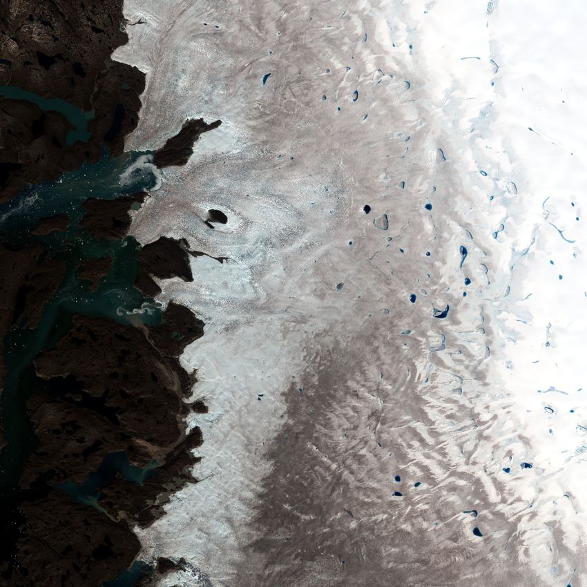
products (Naegeli et al., 2017); this research indicates that Our analysis focuses on a ∼ 12 000 km2 area of West Green-
Sentinel-2 can be reliably combined with Landsat 8 since land, extending ∼ 110 km latitudinally and ∼ 90 km from the
they produce similar results. Thus, Sentinel-2 imagery offers ice margin, with this spatial extent chosen based on the full
great potential for determining the changing volumes of lakes coverage of the original Sentinel-2 tiles (Fig. 1; Sect. 2.2.2).
on the GrIS, for resolving smaller lakes, and for calculating The region is primarily a land-terminating sector of the ice
volumes with higher accuracy than is possible with MODIS sheet, extending from the Sermeq Avannarleq outlet, which
(Williamson et al., 2017). is just north of Jakobshavn Isbræ, near Ilulissat, to just south
In this study, our objective is to present an automatic of Store Glacier in the Uummannaq district. We chose this
method for monitoring the evolution and drainage of lakes study location because it is an area of high lake activity, hav-
on the GrIS using a combination of Sentinel-2 and Landsat 8 ing been the focus of many previous remote-sensing studies
imagery, which will allow the mosaicking of a high-spatial- with which our results can be compared (e.g. Box and Ski,
resolution (10–30 m) record, with a frequent revisit time (ap- 2007; Selmes et al., 2011; Fitzpatrick et al., 2014; Miles et
proaching that of MODIS), something only possible by using al., 2017; Williamson et al., 2017, 2018).
the two sets of imagery simultaneously. The objective is ad-
dressed using four aims, which are as follows. 2.2 Satellite imagery collection and pre-processing
1. We aim to trial new methods for calculating lake areas,
depths, and volumes from Sentinel-2 imagery and as- 2.2.1 Landsat 8
sess their accuracy against Landsat 8 for 2 days of over-
A total of 17 Landsat 8 images from May to Octo-
lapping imagery in 2016.
ber 2016 (Table S2) were downloaded from the USGS
2. We aim to apply the best methods for Sentinel-2 from Earth Explorer interface (http://earthexplorer.usgs.gov, last
(1), alongside existing methods for calculating lake ar- access: 20 September 2018). These were level-1T, ra-
eas, depths, and volumes for Landsat 8, to all of the diometrically and geometrically corrected images, which
available 2016 melt season (May–October) imagery for were distributed as raw digital numbers. We required the
a large study site (∼ 12 000 km2 ) in West Greenland. 30 m resolution data from bands 2 (blue; 0.452–0.512 µm),
The aim is to apply these methods within an automated 3 (green; 0.533–0.590 µm), 4 (red; 0.636–0.673 µm), and
lake-tracking algorithm to produce time series of water- 6 (shortwave infrared (SWIR); 1.566–1.651 µm), and the
www.the-cryosphere.net/12/3045/2018/ The Cryosphere, 12, 3045–3065, 2018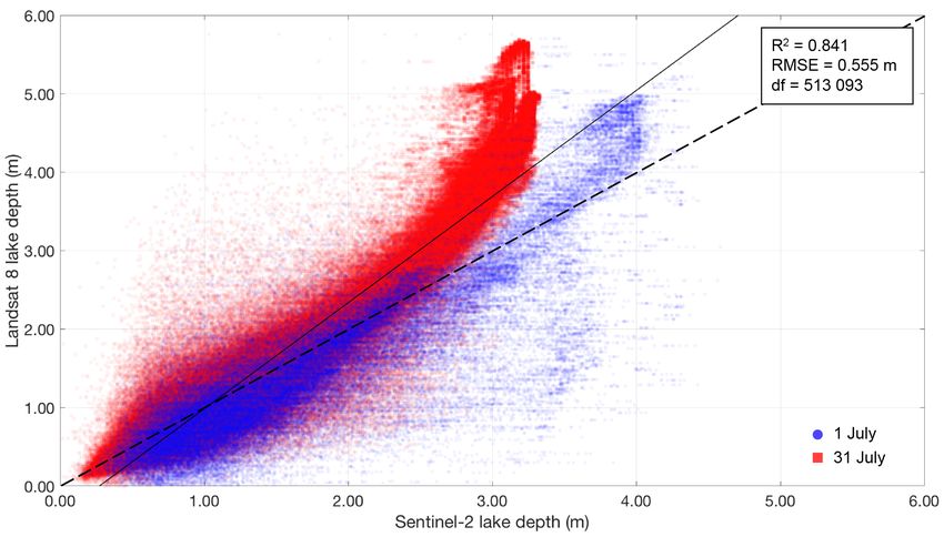
3048                              A. G. Williamson et al.: Dual-satellite remote sensing of supraglacial lakes in Greenland

15 m resolution data from band 8 (panchromatic; 0.503–
0.676 µm). We used all available 2016 imagery that cov-
ered at least a portion of the study site, regardless of
cloud cover. Since Landsat 8 images cover greater areas
than Sentinel-2 images, we batch cropped the Landsat 8
images to the extent of the Sentinel-2 images using Ar-
cGIS’s “Extract by Mask” tool. All of the tiles were re-
projected (using bilinear resampling) to the WGS 84 UTM
zone 22N geographic coordinate system (EPSG: 32622) for
consistency with the Sentinel-2 images, and ice-marginal
areas were removed with the Greenland Ice Mapping
Project (GIMP) ice-sheet mask (Howat et al., 2014). The
raw digital numbers were converted to top-of-atmosphere
(TOA) reflectance using the image metadata and the USGS
Landsat 8 equations (available at: https://landsat.usgs.gov/
landsat-8-l8-data-users-handbook-section-5, last access: 20
September 2018). Landsat 8 TOA values adequately rep-
resent surface reflectance in Greenland (Pope et al., 2016)
and have been used previously for studying GrIS hydrology          Figure 1. The ∼ 12 000 km2 study site within Greenland (in-
(Pope et al., 2016; Miles et al., 2017; Williamson et al., 2017,   set). The background image is a Sentinel-2 RGB image from
2018; Macdonald et al., 2018). Our cloud-masking proce-            11 July 2016 (see Table S1 for image details). The green box and en-
dure involved marking pixels as cloudy when their band-6           larged subplot show a rapidly draining lake and the red circle shows
                                                                   a non-rapidly draining lake (see Fig. 5).
(SWIR) TOA reflectance value exceeded 0.100 (Fig. 2), a
method used for MODIS imagery albeit requiring a higher
threshold value of 0.150 (Williamson et al., 2017). We chose
this lower threshold based on manual inspection of the pixels      Sentinel-2’s 10 m resolution bands 2 (blue; 0.460–0.520 µm),
marked as cloudy against clouds visible on the original im-        3 (green; 0.534–0.582 µm), and 4 (red; 0.655–0.684 µm), and
ages. To reduce any uncertainty in the cloud-filtering tech-       20 m resolution data from band 11 (SWIR; 1.570–1.660 µm).
nique, we then dilated the cloud mask by 200 m (just over          Ice-marginal areas were removed using the GIMP ice-sheet
6 Landsat 8 pixels), so that we could be confident that all        mask (Howat et al., 2014). We used a cloud-masking pro-
clouds and their nearby shadows had been marked as “no             cedure similar to that for Landsat 8, in which pixels were
data” and would not affect the subsequent analyses. The im-        assumed to be clouds and were marked as no data when the
ages were manually checked for shadowing elsewhere, with           TOA value exceeded a threshold of 0.140 in band 11 (SWIR),
any shadows filtered where present.                                after the band-11 data had been interpolated (using nearest-
                                                                   neighbour resampling) to 10 m resolution for consistency
2.2.2   Sentinel-2                                                 with the optical bands (Fig. 2). This threshold was chosen by
                                                                   manually comparing the pixels identified as clouds against
A total of 39 Sentinel-2A level-1C images from May to              background RGB images. As with the Landsat 8 images, we
October 2016 (Table S1) were downloaded from the Ama-              dilated the cloud mask by 200 m (10 Sentinel-2 pixels) to ac-
zon S3 Sentinel-2 database (http://sentinel-pds.s3-website.        count for any uncertainty in the cloud-masking procedure,
eu-central-1.amazonaws.com, last access: 20 September              and again the images were manually checked for shadowing
2018). The Sentinel-2 data were distributed as TOA re-             elsewhere, with any shadows filtered where present.
flectance values that were radiometrically and geometrically
corrected, including ortho-rectification and spatial registra-     2.3   Lake area delineation
tion to a global reference system with sub-pixel accuracy. We
note that Sentinel-2 and Landsat 8 images are ortho-rectified      Figure 2 summarises the overall method used to calculate
using different DEMs, which may produce slight offsets in          lake areas and depths for the Landsat 8 and Sentinel-2
lake locations (Kääb et al., 2016; Paul et al., 2016); two con-    imagery, including the cloud-masking procedure described
temporaneous image pairs (1 July and 31 July 2016) were            above, and the resampling required because the data were
therefore manually checked prior to analysis, but no obvi-         distributed at different spatial resolutions. We derived lake
ous offset was observed. We included all Sentinel-2 images         areas for the two sets of imagery using the normalised differ-
from 2016 that had ≥ 20 % data cover of the study region and       ence water index (NDWI) approach, which has been widely
≤ 75 % cloud cover. This resulted in using 39 images from          used previously for medium- to high-resolution imagery of
the 77 in total available in 2016, reducing the average tempo-     the GrIS (e.g. Moussavi et al., 2016; Miles et al., 2017).
ral resolution from 2.0 to 3.9 days. We downloaded data from       There were two stages involved here. First, we applied vari-

The Cryosphere, 12, 3045–3065, 2018                                                     www.the-cryosphere.net/12/3045/2018/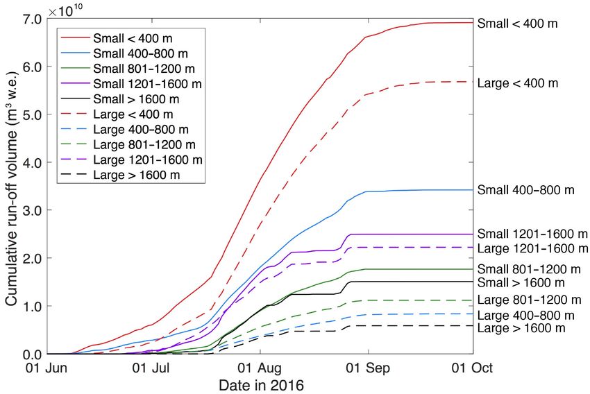
A. G. Williamson et al.: Dual-satellite remote sensing of supraglacial lakes in Greenland                                                                                3049

         Sentinel-2                                                  Cloud
                                                                     mask                                                                     Landsat 8
                                           Apply cloud            Resample to                       Apply cloud                       Cloud             Resample to
                                             mask                  10 m (NN)                          mask                            mask               15 m (NN)

                                          Apply GIMP              Clouds when                       Apply GIMP                     Clouds when           Apply cloud
                                           ice mask               value > 0.140                      ice mask                      value > 0.100           mask

                             Red                 Blue    Green       SWIR             Red                 Blue             Green      SWIR              Panchromatic

                                   NDWI (0.25                                               NDWI (0.25                                                  Resample to
                                    threshold)                                               threshold)                                                  30 m (B)

                                     Lake                                                     Lake                                                      Calculate lake
                                     areas                                                    areas                                                      depth (PB)

                     Calculate lake                                                                                 Resample to       Lake
                      depth (PB)                                                                                     10 m (NN)        areas

                         Lake                                                     Calculate lake                     Average PB
                        depths                                                     depth (PB)                        lake depths

                                                                                                                        Lake       Resample to              Lake
                                                                                                                       depths       10 m (NN)              depths

                     Input                Process        Output                   Input / output spatial resolution (m):      10     15            20         30

Figure 2. Summary of the methods applied to the Sentinel-2 and Landsat 8 input data to calculate lake areas using the NDWI and depths
using the physically based (“PB” in this figure) method. In this figure, the interpolation techniques used are indicated by “NN” for nearest
neighbour or “B” for bilinear. The methods applied to Landsat 8 are shown only once the images had been reprojected and batch cropped to
the same extent as the Sentinel-2 images (Sect. 2.2.1). The lake area outputs are compared between the two datasets as described in Sect. 2.3,
and the physically based lake depth outputs are compared as outlined in Sect. 2.4. When the empirical lake depth method for calculating
Sentinel-2 lake depths was also evaluated, the final Landsat 8 depths at 10 m resolution were directly compared against the original Sentinel-2
input band data (at native 10 m resolution) within the lake outlines defined with the NDWI.

ous NDWI thresholds to the Sentinel-2 and Landsat 8 images                        of < 5 pixels in total and linear features < 2 pixels wide
and compared the delineated lake boundaries against the lake                      since these were likely to represent areas of mixed slush or
perimeters in the background RGB images. We then qualita-                         supraglacial streams, as opposed to lakes (Pope, 2016; Pope
tively selected the NDWI threshold for each type of imagery                       et al., 2016).
based on the threshold that produced the closest match be-
tween the two. Based on this qualitative analysis, we chose                       2.4       Lake depth and volume estimates
NDWI thresholds of 0.25 for both types of imagery (Fig. 2).
By varying the thresholds from these values to 0.251 and                          2.4.1       Landsat 8
0.249, the total lake area calculated across the whole im-
age only changed by < 2 %. The second stage involved com-                         For each Landsat 8 image, we calculated the lake depths and
paring the areas of 594 lakes defined using the NDWI for                          volumes using the physically based method of Pope (2016)
the contemporaneous Landsat 8 and Sentinel-2 images from                          and Pope et al. (2016), based on the original method for
1 July (collected within < 90 min of each other) and 31 July                      ASTER imagery from Sneed and Hamilton (2007). This ap-
(collected within < 45 min of each other). This gave an ex-                       proach is based on the premise that there is a measurable
tremely close agreement between the two sets of lake areas                        change in the reflectance of a pixel within a lake according to
(R 2 = 0.999; RMSE = 0.007 km2 , equivalent to 7 Sentinel-2                       its depth since deeper water causes higher attenuation of the
pixels) without any bias, so we were confident that the NDWI                      optical wavelengths within the water column. Lake depth (z)
approach applied to the two types of imagery reproduced the                       can therefore be calculated based on the satellite-measured
same lake areas (Fig. S1). Using these NDWI thresholds,                           reflectance for a pixel of interest (Rpix ) and other lake prop-
we created binary (i.e. lake and non-lake) masks for each                         erties:
day of imagery for the two satellites. Since the Landsat 8                               [ln (Ad − R∞ ) − ln(Rpix − R∞ )]
optical-band data were at 30 m native resolution, we resam-                       z=                                      ,                                               (1)
                                                                                                        g
pled them to 10 m resolution (using nearest-neighbour re-
sampling) for consistency with the resolution of the Sentinel-                    where Ad is the lake-bottom albedo, R∞ is the reflectance
2 data (Fig. 2). From the binary images, we removed groups                        for optically deep (> 40 m) water, and g is the coefficient for

www.the-cryosphere.net/12/3045/2018/                                                                                The Cryosphere, 12, 3045–3065, 2018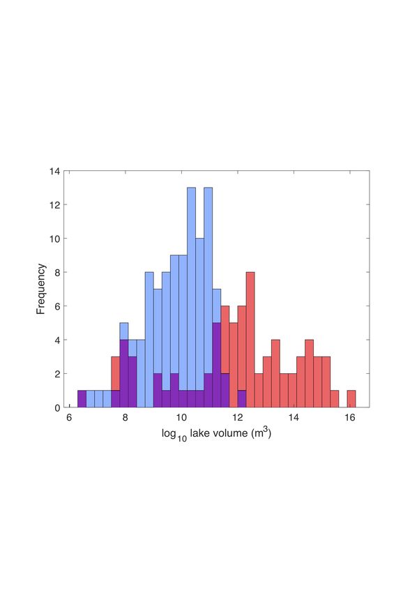
3050                              A. G. Williamson et al.: Dual-satellite remote sensing of supraglacial lakes in Greenland

the losses in upward and downward travel through a water           (independent variables) for each pixel within the lake out-
column. For Landsat 8, we followed the recommendation of           lines predicted in both sets of imagery to determine which
Pope et al. (2016), taking an average of the depths calculated     band and relationship produced the best match between the
using the red and panchromatic band TOA reflectance data           two datasets. To compare these values, we first resampled
within the boundaries of the lakes (before they had been re-       (using nearest-neighbour interpolation) the Landsat 8 depth
sampled to 10 m resolution for comparing the Sentinel-2 and        data from 30 to 10 m to match the resolution of the Sentinel-2
Landsat 8 lake areas; Sect. 2.3) defined by the method de-         TOA reflectance data (Fig. 2).
scribed in Sect. 2.3. Since the panchromatic-band data were           To evaluate the performance of the empirical versus phys-
at 15 m resolution, we resampled them using bilinear interpo-      ical techniques, we calculated goodness-of-fit indicators for
lation to match the 30 m red-band resolution (Fig. 2). Ad was      the Sentinel-2 and Landsat 8 measurements derived from the
calculated as the average reflectance in the relevant band for     empirically based technique (applied to all optical bands) and
the ring of pixels immediately surrounding a lake, R∞ was          physically based method (applied to the red and green bands)
determined from optically deep water in proglacial fjords on       for the two validation dates (1 and 31 July 2016) when con-
a scene-by-scene basis for each band, and we used g val-           temporaneous Landsat 8 and Sentinel-2 images were avail-
ues for the relevant Landsat 8 bands from Pope et al. (2016).      able.
Lake volume was calculated as the sum of lake depths, mul-            As for Landsat 8, Sentinel-2 lake volumes were calculated
tiplied by the pixel area, within the lake outlines. We treated    as the sum of the individual lake depths, multiplied by the
these Landsat 8 depths and volumes as ground-truth data as         pixel areas, within the lake boundaries.
in Williamson et al. (2017).
                                                                   2.5     Lake evolution and rapid-lake-drainage
2.4.2   Sentinel-2                                                         identification

Since no existing work has derived lake depths using               2.5.1    Time series of lake water volumes
Sentinel-2, we needed to formulate a new method. For this
purpose, we used the Landsat 8 lake depths as our validation       Once validated, the new techniques to calculate lake areas,
dataset. We conducted the validation on the two dates (1 and       depths, and volumes from Sentinel-2, as well as the exist-
31 July 2016) with contemporaneous Landsat 8 and Sentinel-         ing methods for Landsat 8 (Sect. 2.4), were applied to the
2 images (as described in Sect. 2.3). We chose to test both        satellite imagery within the Fully Automated Supraglacial
physically based and empirically based techniques to derive        lake Tracking at Enhanced Resolution (FASTER) algorithm
Sentinel-2 lake depths, noting at the outset that physical tech-   to produce cloud- and ice-marginal-free 10 m resolution lake
niques are generally thought to be preferable over empirical       area and depth arrays for each day of the 2016 melt season for
ones since they do not require site- or time-specific tuning.      which either a Landsat 8 or Sentinel-2 image was available
   For the physically based technique, we tested whether           (Fig. 2). For the days (1 and 31 July) when both Landsat 8
the same method as applied to Landsat 8 (Eq. 1) could              and Sentinel-2 imagery was available (as used for the com-
be used on the Sentinel-2 TOA reflectance data. However,           parisons above), in the FASTER algorithm, we used only the
since Sentinel-2 does not collect panchromatic band mea-           higher-resolution Sentinel-2 images. The FASTER algorithm
surements, we could only use individual Sentinel-2 bands to        is an adapted version of the Fully Automated Supraglacial
calculate lake depths. We applied this physically based tech-      lake Tracking (FAST) algorithm (Williamson et al., 2017),
nique to the red- and green-band data within the lake outlines     which was developed for MODIS imagery. The FASTER al-
defined with the NDWI (Sect. 2.3). We derived the value for        gorithm involves creating an array mask to show the max-
R∞ as described above for Landsat 8. Since the lake depth          imum extent of lakes within the region in the 2016 melt
calculations are particularly sensitive to the Ad value (Pope      season, by superimposing the lake areas from each image.
et al., 2016), it was critical to ensure that the lake-bottom      Within this maximum lake-extent mask, changes to lake ar-
albedo was correctly identified. Thus, to define Ad , we di-       eas and volumes were tracked between each consecutive im-
lated the lake by a ring of 2 pixels, and not 1, to ensure that    age pair, with any lakes that were obscured (even partially)
shallow water was not included due to the finer pixel resolu-      by cloud marked as no data. We only tracked lakes that grew
tion and due to any errors in the lake outlines derived using      to ≥ 495 pixels (i.e. 0.0495 km2 ) at least once in the sea-
the NDWI. We also calculated new g values for Sentinel-2’s         son, which is identical to the minimum threshold used by
red and green bands using the methods of Pope et al. (2016)        Miles et al. (2017), and is based on the minimum estimated
(Sect. S1).                                                        lake size (approximated as a circle) required to force a frac-
   Our empirically based approach involved deriving vari-          ture to the ice-sheet bed (Krawczynski et al., 2009). It is en-
ous lake depth–reflectance regression relationships to deter-      couraging that this minimum threshold size for lake tracking
mine which explained the most variance in the data. We used        was over 7 times larger than the error (0.007 km2 ) associated
the Landsat 8 lake depth data (dependent variable) and the         with calculating lake area (Sect. 2.3; Fig. S1). While a lower
Sentinel-2 TOA reflectance data for the three optical bands        tracking threshold could have been used, it would have sig-

The Cryosphere, 12, 3045–3065, 2018                                                    www.the-cryosphere.net/12/3045/2018/
A. G. Williamson et al.: Dual-satellite remote sensing of supraglacial lakes in Greenland 3051
nificantly increased computational time and power required, each rapidly draining lake was delineated using MATLAB’s
alongside adding uncertainty to whether the tracked groups “watershed” function, applied to the GIMP ice-surface el-
of pixels actually represented lakes. This tracking procedure evation data (Howat et al., 2014). The elevation data were
produced time series for all lakes to show their evolution over first coarsened using bilinear resampling to 100 m resolu-
the whole 2016 melt season. tion from 30 m native resolution. For each of the days after
rapid lake drainage had finished, it was assumed that all of
2.5.2 Rapid-lake-drainage identification the run-off within a lake’s catchment reached the moulin in
that catchment instantaneously (i.e. no flow-delay algorithm
From the time series, a lake was classified as draining rapidly was applied) and entered the GrIS. This method therefore as-
if two criteria were met: (i) it lost > 80 % of its maximum sumes that once a moulin has opened at a lake-drainage site,
seasonal volume in ≤ 4 days (following Doyle et al., 2013; it remains open for the remainder of the melt season. This
Fitzpatrick et al., 2014; Miles et al., 2017; Williamson et allowed first-order comparisons between cumulative run-off
al., 2017, 2018), and (ii) it did not then refill on the sub- routed into the GrIS via the moulins opened by small and
sequent day of cloud-free imagery by > 20 % of the total large lake-drainage events.
water volume lost during the previous time period (follow-
ing Miles et al., 2017); the aim here was to filter false pos-
itives from the record. However, we also tested the sensi- 3 Results
tivity of the rapid-lake-drainage identification methodology
by varying the threshold by ±10 % (i.e. 70 %–90 %) for the 3.1 Sentinel-2 lake depth estimates
critical-volume-loss threshold, ±10 % (i.e. 10 %–30 %) for
the critical-refilling threshold, and ±1 day (i.e. 3–5 days) for Table 1 shows the results of the lake depth calculations
the critical-timing threshold. using the physically and empirically based techniques ap-
To determine how much extra information could be ob- plied to imagery from 1 and 31 July 2016 when contem-
tained from the finer-spatial-resolution satellite record, we poraneous Landsat 8 and Sentinel-2 images were available.
compared the number of rapidly draining lakes identified The physically based method applied to the red and green
that grew to ≥ 0.125 km2 (which would be resolvable by bands (Figs. 3 and S2, respectively) performed slightly worse
MODIS) with the number that never grew to this size (which (for the red band: R 2 = 0.841 and RMSE = 0.555 m; for the
would not be resolvable by MODIS) at least once in the sea- green band: R 2 = 0.876 and RMSE = 0.488 m) than the best
son. We defined the drainage date as the midpoint between empirical method (Fig. 4) when a power-law regression was
the date of drainage initiation and cessation and identified applied to the data (R 2 = 0.889 and RMSE = 0.447 m). Fig-
the precision of the drainage date as half of this value. We ures S3 and S4 respectively show the data for the empiri-
conducted three sets of analyses: one for each set of imagery cal technique applied to the Sentinel-2 TOA reflectance and
individually and a third for both sets together; the intention Landsat 8 lake depths for the worse-performing Sentinel-2
here was to quantify how mosaicking the dual-satellite record green and blue bands (Table 1). The physically based method
improved the identification of lake-drainage events compared applied to the red-band data performed better on 1 July,
with using either record alone. The water volumes reaching when the relationship between Sentinel-2-derived depths and
the GrIS’s internal hydrological system from the small and Landsat 8 depths was more linear (Fig. 3, blue markers)
large lakes during the drainage events themselves were de- than on 31 July (Fig. 3, red markers), when the relationship
termined using the lake-volume measurements on the day of was more curvilinear. This is because the depths calculated
drainage. with Sentinel-2 on 31 July were limited to ∼ 3.5 m, while
higher depths (> 4 m) were reported on 1 July (Fig. 3). Al-
2.6 Run-off deliveries following moulin opening though less distinct, the best empirical relationship also dif-
fered slightly in performance between the two dates (Fig. 4).
Using the dual Sentinel-2 and Landsat 8 record, the loca- Section 4.1 discusses the possible reasons for the under-
tions and timings of moulin openings by “large” and “small” measurement of lake depths with Sentinel-2 on 31 July com-
rapidly draining lakes were identified. Then, at these moulin pared with 1 July. The physically based method applied
locations, the run-off volumes that subsequently entered the to the green-band data performed similarly on both vali-
ice sheet were determined using statistically downscaled dation dates (Fig. S2). Although application of the physi-
daily 1 km resolution RACMO2.3p2 run-off data (Noël et cally based technique to the green band produced a slightly
al., 2018). Here, run-off was defined as melt plus rainfall mi- higher R 2 and lower RMSE compared with the physically
nus any refreezing in snow (Noël et al., 2018). These data based method applied to the red-band data, the depths es-
were reprojected from Polar Stereographic (EPSG: 3413) to timated with Sentinel-2 were unrealistically high compared
WGS 84 UTM zone 22N (EPSG: 32622) for consistency with those from Landsat 8: Sentinel-2 reports a maximum
with the other data and resampled to 100 m resolution us- depth of ∼ 19 m, comparing with an equivalent value of
ing bilinear resampling. Then, the ice-surface catchment for ∼ 5.5 m for Landsat 8 (Fig. S2). This produced more scatter
www.the-cryosphere.net/12/3045/2018/ The Cryosphere, 12, 3045–3065, 20183052 A. G. Williamson et al.: Dual-satellite remote sensing of supraglacial lakes in Greenland
Table 1. Goodness-of-fit indicators for the empirical and physical techniques tested in this paper for deriving Sentinel-2 lake depths, with
validation against the Landsat 8 lake depth measurements, on 1 and 31 July 2016. R 2 is the coefficient of determination, RMSE is the
root-mean-square error, SSE is the sum of squares due to error, and OLS is ordinary least squares. The best performing (red band) regression
relationship (i.e. the one with the highest R 2 and lowest RMSE and SSE) among the empirical techniques is shown in italicised text. Data for
the physical relation applied to Sentinel-2’s green band are presented in Fig. S2, and data for the empirical relation applied to Sentinel-2’s
green and blue bands are presented in Figs. S3 and S4, respectively.
Sentinel-2 Goodness-of-fit OLS Power-law Exponential
band indicator regression regression regression
(technique)
Red R2 0.702 0.889 0.842
(empirical) RMSE 0.734 0.448 0.534
SSE (m3 ) 2.39 × 10⁵ 8.62 ×10⁴ 1.23 × 10⁵
Green R2 0.782 0.768 0.829
(empirical) RMSE 0.627 0.647 0.556
SSE (m3 ) 1.69 × 10⁵ 1.80 × 10⁵ 1.33 × 10⁵
Blue R2 0.647 0.622 0.673
(empirical) RMSE 0.799 0.826 0.768
SSE (m3 ) 2.75 × 10⁵ 2.94 × 10⁵ 2.54 × 10⁵
Red R2 0.841 – –
(physical) RMSE 0.555
SSE (m3 ) 1.58 × 10⁵
Green R2 0.876 – –
(physical) RMSE 0.488
SSE (m3 ) 1.22 × 10⁵
Figure 3. Comparison of lake depths calculated using the physically based method for Sentinel-2 (with the red band) and for Landsat 8 (with
the average depths from the red and panchromatic bands). Degrees of freedom (“df” in this figure) = 513 093. The solid black line shows an
ordinary least-squares (OLS) linear regression and the dashed black line shows a 1 : 1 relation. The R 2 value indicates that the regression
explains 84.1 % of the variance in the data. The RMSE of 0.555 m shows the error associated with calculating the Sentinel-2 lake depths
using this relationship.
The Cryosphere, 12, 3045–3065, 2018 www.the-cryosphere.net/12/3045/2018/A. G. Williamson et al.: Dual-satellite remote sensing of supraglacial lakes in Greenland 3053
Figure 4. The empirical power-law regression (solid black curve, equation y = 0.2764x −0.8952 ) between Sentinel-2 red-band TOA re-
flectance and Landsat 8 lake depth. Degrees of freedom (“df” in this figure) = 430 650. The R 2 value indicates that the regression explains
88.9 % of the variance in the data. The RMSE of 0.447 m shows the error associated with calculating the Sentinel-2 lake depths using this
relationship.
for the green-band than the red-band physical method (Ta- 9.0 days (for Landsat 8) and 3.9 days (for Sentinel-2) to
ble 1). 2.8 days (for the dual-satellite record). The months of June
Although the physically based method performed slightly and July had the most imagery available (both with 14 im-
worse than the empirical techniques, the physical method is ages) within the dual-satellite analysis. For the Landsat 8 in-
preferable because it can be applied across wide areas of the dividual analysis, the algorithm tracked changes to 453 lakes
GrIS and in different years without site- or time-specific tun- that grew to ≥ 0.0495 km2 once in the season; equivalent
ing; it is likely that a different empirical relationship would numbers were 599 lakes for the Sentinel-2 analysis and 690
have better represented the data for a different area of the lakes for the dual-satellite analysis. Using the dual-satellite
GrIS or in a different year. We therefore carried forward record therefore involved tracking an additional 237 (or 91)
the physically based method applied to the red band into lakes over the season than was possible with Landsat 8 (or
the lake-tracking approach. We selected the red band instead Sentinel-2) alone.
of the green band because of the large difference between The largest lake size varied between the analyses: 4.0 km2
the depths calculated with the two satellites at higher val- for Landsat 8 (recorded on 16 July 2016) and 8.6 km2 for
ues when using the green band (Fig. S2). We defined the Sentinel-2 (recorded on 21 July 2016), which may be be-
error on all of the subsequently calculated lake depth (and cause there were no Landsat 8 images close to 21 July 2016.
therefore lake volume) measurements for Sentinel-2 using The maximum lake volumes recorded also varied between
the RMSE of 0.555 m and treated the Landsat 8 measure- the two platforms: 1.1 × 10⁷ m3 for Landsat 8 (recorded on
ments as ground-truth data, meaning they did not have errors 15 July 2016) and 1.2 × 10⁷ m3 for Sentinel-2 (recorded on
associated with them. 14 July 2016). The mean lake size across all of the images
from the dual Sentinel-2–Landsat 8 record was 0.137 km2
3.2 Lake evolution (25th and 75th percentiles = 0.0075 and 0.129 km2 , respec-
tively). This value is therefore just above (by 0.012 km2 )
Having verified the reliability of the lake area and depth tech- the threshold reporting size of MODIS, assuming 2 250 m
niques for both Sentinel-2 and Landsat 8, the automatic cal- MODIS pixels are required to confidently classify lakes
culation methods were included in the FASTER algorithm (Fitzpatrick et al., 2014; Williamson et al., 2017). Unpaired
to derive seasonal changes to lake areas and depths, and Student’s t tests between Sentinel-2 and Landsat 8 lake ar-
therefore volumes. The FASTER algorithm was applied to eas and volumes (from all of the imagery) confirmed that
the Landsat 8 and Sentinel-2 image batches individually, they were not significantly different with > 99 % confidence
as well as to both sets when combined into a dual-satellite (t = 6.5, degrees of freedom = 9503 for areas; t = 11.4, de-
record. Using the dual-satellite image collection produced an grees of freedom = 6859 for volumes), justifying using the
improvement to the temporal resolution of the dataset over two imagery types together despite their resolution difference
the melt season (1 May to 30 September) from averages of (10 m vs. 30 m).
www.the-cryosphere.net/12/3045/2018/ The Cryosphere, 12, 3045–3065, 20183054 A. G. Williamson et al.: Dual-satellite remote sensing of supraglacial lakes in Greenland
10 5
5.0
(a)
4.0
Lake volume (m3)
3.0
2.0
1.0
volume (m3)
0.0
01-May
10
6 01-Jun 01-Jul 01-Aug 01-Sep 01-Oct
5.0 Date in 2016
(b)
Lake volume (mLake
4.0
3
)
3.0
2.0
1.0
0.0
01 May 01 Jun 01 Jul 01 Aug 01 Sep 01 Oct
Date in 2016
Figure 5. Sample time series of lake volume to show seasonal changes for (a) a non-rapidly draining lake (Fig. 1, red circle) and (b) a rapidly
draining lake (Fig. 1, green box). Lines connect points without any data smoothing. Error bars were calculated by multiplying the lake depth
RMSE of 0.555 m (Sect. 3.1) by the pixel size and the number of pixels in the lake on each image.
10 8
Portion of region visible (%)
100 150.0
Total lake volume (m3)
Total lake area (km2)
2.0
80
100.0 1.5
60
1.0
40
50.0
20 0.5
0 0.0 0.0
01 May 01 Jun 01 Jul 01 Aug 01 Sep 01 Oct
Date in 2016
7
10
150.0 15.0 )
Figure 6. Evolution to total lake area and volume across the whole study region during the 2016 melt season. “Portion of region visible”
measures the percentage of all of the pixels within the entire region that are visible in the satellite image, i.e. which are not obscured either
by cloud (or cloud shadows) or are not missing data values. Figure 7 presents total lake area and volume after normalising for the proportion
of region visible. Blue error bars for lake area were calculated by multiplying the lake area RMSE of 0.007 km2 (Sect. 2.3) by the number
of lakes identified on each image; red error bars for total lake volume were calculated by multiplying the lake depth RMSE of 0.555 m
(Sect. 3.1) by the pixel size and the number of pixels identified as water covered in each image.
Using the full Sentinel-2–Landsat 8 dataset, the FASTER evolution on the GrIS: there was virtually no water in lakes
algorithm produced time series that documented changes to before June, steady increases in total lake area and volume
individual lake volumes over the season, samples of which until the middle of July, and then a gradual decrease in to-
are shown in Fig. 5. Total areal and volumetric changes tal lake area and volume through the remainder of the sea-
across the whole region were calculated by summing the val- son, with most lakes emptying by early September (Figs. 6
ues for all lakes in the region. However, we found that cloud and 7). Dates with seemingly low total lake areas and vol-
cover (which was masked from the images) often affected umes were usually explained by the low portion of the whole
the observational record, and there were time periods, such region visible in those images (Figs. 6 and 7). Finally, as in
as early July and the end of August, with a lot of missing previous studies (e.g. Box and Ski, 2007; Georgiou et al.,
data (Fig. 6). Figure 7 was therefore produced to normalise 2009; Williamson et al., 2017), we found a close correspon-
total lake areas and volumes against the proportion of the dence between lake areas and volumes: comparing lake area
region visible, and this shows the estimated pattern of lake
The Cryosphere, 12, 3045–3065, 2018 www.the-cryosphere.net/12/3045/2018/A. G. Williamson et al.: Dual-satellite remote sensing of supraglacial lakes in Greenland 3055
and volume values from all dates produced an R 2 value of (range = 0.006–91.0 × 10⁵ m3 ; σ = 10.2 × 10⁵ m3 ) into the
0.73 (p = 1.03 × 10⁻¹⁰ ). ice sheet (Table 2; Fig. 9). Figure 9 shows the patterns
of run-off delivery across the region, suggesting that small
3.3 Rapid lake drainage (< 0.125 km2 ) and large (≥ 0.125 km2 ) rapidly draining
lakes were randomly distributed across the region, although
Table 2 shows the results of the identification of rapidly there were more numerous smaller lakes at lower elevations
draining lakes using the three different datasets and indicates in the north. Figure 10 shows that large lakes generally con-
that the dual-satellite record was better for identifying rapidly tained more water than small lakes, as might be expected, but
draining lakes than the individual records. This was for two also shows that large lakes contained a higher range of water
main reasons. First, the dual-satellite record identified 118 volumes than small lakes, producing an overlap between the
(or 91) more rapidly draining lakes than the Landsat 8 (or lake types for the lower water volume values. Thus, although
Sentinel-2) record in isolation (Table 2). When either record large lakes each covered a higher area, some large lakes must
was used alone, Sentinel-2 (or Landsat 8) performed better have been relatively shallow, as also suggested by the red to
(or worse), identifying 50.5 % (or 35.9 %) of the total num- yellow coloured triangles in Fig. 9.
ber of rapidly draining lakes identified by the dual-satellite Using the data from the dual-satellite record, and consid-
record. Second, with the dual-satellite dataset, drainage dates ering just the water volumes delivered into the GrIS during
were identified with higher precision (i.e. half of the number lake-drainage events (and not subsequently via the moulins
of days between the date of drainage initiation and cessa- opened), the drainage of small (< 0.125 km2 ) lakes deliv-
tion; Sect. 2.5.2) than with the Sentinel-2 analysis (Table 2). ered a total run-off volume of 31.2 × 10⁵ m3 into the GrIS,
However, the precision appears higher for the Landsat 8 anal- which is just 5.1 % of the total volume (617.3 × 10⁵ m3 ) de-
ysis than either the dual-satellite or Sentinel-2 analysis, and livered into the GrIS during the drainage of all lakes across
this is because nearly all Landsat 8 lake-drainage events oc- the region (Table 2). Although this volume is low, small lake-
curred on two occasions when the pair of images was only drainage events, like large lake-drainage events, are addition-
separated by a day, on 8–9 July (small lakes) and 13–14 July ally important because they are associated with the opening
(large lakes) (Table 2). of moulins that transport surface run-off into the GrIS, and
The dual-satellite record also identified the rapid drainage perhaps to the bed, for the remainder of the season, assum-
of many small lakes (< 0.125 km2 ) that would not be vis- ing that the moulin remains open (e.g. Banwell et al., 2016;
ible with MODIS imagery due to the lower limit of its re- Koziol et al., 2017). Associating lake drainages with moulin
porting size (Table 2), thus presenting an advantage of the opening in this way means that the dual-satellite record found
dual-satellite record over the MODIS record of GrIS surface an additional 105 moulins (Table 2) that would not have been
hydrology. These smaller lakes tended to drain rapidly ear- identified by MODIS; this is greater than the total number of
lier in the season (mean date = 8 July for the dual-satellite moulins associated with large lake-drainage events (79) that
record) than the larger lakes (mean date = 11 July for the could have been identified by MODIS, assuming MODIS
dual-satellite record), although the difference in dates is can identify all lakes > 0.125 km2 , which itself is unlikely
small, with most lakes draining in early to mid-July (Table 2; (Leeson et al., 2013; Williamson et al., 2017). Figure 11
Fig. 8). In general, lakes closer to the ice margin tended to shows that the moulins opened by the rapid drainage of small
drain earlier than those inland (Fig. 8). lakes allowed a higher total volume of run-off to enter the
Finally, we tested how adjusting the thresholds used to de- GrIS than that routed via moulins opened by rapidly drain-
fine rapidly draining lakes would impact rapid-lake-drainage ing large lakes; in total, moulins opened by small (or large)
identification. Changing the critical volume loss required lakes channelled 1.61 × 10¹¹ (or 1.04 × 10¹¹ ) m3 of run-off
for a lake to be identified as having drained from 80 % to into the GrIS’s internal hydrological system. Thus, moulins
70 % and 90 % resulted in the identification of only six more opened by small (or large) lakes delivered 61.5 % (or 38.5 %)
and four fewer rapid-lake-drainage events, respectively. Sim- of the total run-off into the GrIS after opening. Moreover,
ilarly, changing the critical-refilling threshold from 20 % to moulins opened by small lakes delivered more run-off into
10 % and 30 % resulted in identifying only eight fewer and the GrIS than those opened by large lakes across all ice-
five more rapidly draining lakes. However, adjusting the tim- elevation bands, although this finding is more pronounced
ing over which this loss was required had a larger impact, at lower elevations than higher elevations, i.e. below and
with adjustments from 4 to 3 and 5 days producing 37 fewer above 800 m a.s.l. respectively (Fig. 11). The run-off into
and 65 more rapid-lake-drainage events, respectively. the moulins opened by small lakes also tended to reach the
GrIS’s internal hydrological system earlier in the season than
3.4 Run-off deliveries and moulin opening by rapid that delivered into the moulins opened by large lakes because
lake drainage these small lakes tended to drain slightly earlier (Fig. 11).
Each rapid-lake-drainage event from the dual-satellite
record delivered a mean water volume of 3.4 × 10⁵ m3
www.the-cryosphere.net/12/3045/2018/ The Cryosphere, 12, 3045–3065, 20183056 A. G. Williamson et al.: Dual-satellite remote sensing of supraglacial lakes in Greenland
150.0
150.0
area) (km2)
Total lake area (km2)
150.0
100.0
100.0
(a)
2
lake (km
lake area
100.0
50.0
50.0
Total Total 50.0
0.00.0
01-May
01-May 01-Jun
01-Jun 01-Jul
01-Jul 01-Aug
01-Aug 01-Sep
01-Sep 01-Oct
01-Oct
0.0 Date
Date in 2016
in 2016
8
10 810
2.0 Date in 2016
Total lake volume (m )
3
2.0
1.5
10
8
(b)
1.5
1.0
1.0
0.5
0.5
0.0
01 May
1-M 01 nJun
01-J 01 lJul
01-J 01 Aug
01-A g 01 Sep
01-S p 01 Oct
01-Oct
To
0.0 Date
Date in 2016
in 2016
01-May 01-Jun 01-Jul 01-Aug 01-Sep 01-Oct
Date in 2016
Figure 7. Estimates of evolution to total lake (a) area and (b) volume across the whole study region during the 2016 melt season after daily
values were normalised against the proportion of the region visible on that day (i.e. not obscured by cloud or missing data). Values are derived
by dividing the daily total lake area and volume by the portion of the region visible on that day (see Fig. 6).
Table 2. Properties of rapid-lake-drainage events identified using the satellite datasets individually and as part of a dual-satellite dataset. Large
lakes are defined as ≥ 0.125 km2 (identifiable by MODIS), while small lakes are defined as < 0.125 km2 (omitted by MODIS). “DoY” refers
to the day of year in 2016.
Analysis type Property Large lakes Small lakes Total/overall
Sentinel-2 Number of drainage events 45 48 93
Percentage of total lakes 7.5 8.0 15.5
Mean drainage date (DoY) ± mean precision 193.4 ± 1.8 188.2 ± 1.6 190.7 ± 1.7
Minimum drainage volume (105 m3 ) 0.020 0.006 0.006
Maximum drainage volume (105 m3 ) 90.1 2.1 90.1
Mean drainage volume (105 m3 ) 7.5 0.2 3.7
Median drainage volume (105 m3 ) 1.3 0.2 0.3
Total drainage volume (105 m3 ) 337.3 11.7 349.0
Landsat 8 Number of drainage events 30 36 66
Percentage of total lakes 6.6 7.9 14.6
Mean drainage date (DoY) ± mean precision 196.8 ± 0.6 190.5 ± 0.5 193.4 ± 0.5
Minimum drainage volume (105 m3 ) 0.100 0.050 0.050
Maximum drainage volume (105 m3 ) 19.8 1.1 19.8
Mean drainage volume (105 m3 ) 4.2 0.4 2.1
Median drainage volume (105 m3 ) 1.6 0.4 0.6
Total drainage volume (105 m3 ) 126.8 14.1 140.9
Dual Number of drainage events 79 105 184
Sentinel-2 Percentage of total lakes 11.4 15.2 26.7
and Mean drainage date (DoY) ± mean precision 193.1 ± 1.1 190.1 ± 1.0 191.4 ± 1.1
Landsat 8 Minimum drainage volume (105 m3 ) 0.006 0.007 0.006
Maximum drainage volume (105 m3 ) 91.0 1.6 91.0
Mean drainage volume (105 m3 ) 7.4 0.3 3.4
Median drainage volume (105 m3 ) 1.8 0.2 3.9
Total drainage volume (105 m3 ) 586.1 31.2 617.3
The Cryosphere, 12, 3045–3065, 2018 www.the-cryosphere.net/12/3045/2018/A. G. Williamson et al.: Dual-satellite remote sensing of supraglacial lakes in Greenland 3057
19 Jun
Large lakes
2
Small lakes
1 Jul
4
13 Jul
6
Date in 2016
25 Jul
8
6 Aug
10
18 Aug
12
30 Aug
10 km
14
Small lake Large lake 0.5 0.6 0.7 0.8 0.9 1 ln lake volume (m3)
Figure 8. Dates of rapid drainage events for small (circles) and large Figure 10. Frequency distribution of water volumes prior to rapid
(triangles) lakes in 2016. The panel coverage and background are drainage for small and large lakes to show the lower and more
the same as that shown in Fig. 1. The extreme colour bar values tightly clustered water volumes contained within small lakes com-
include those dates outside of the range shown (i.e. before 19 June pared with large lakes. Natural logs of water volumes were taken
and after 5 September). for presentation purposes.
Figure 11. Cumulative run-off volume, from RACMO2.3p2 data
(Noël et al., 2018), entering the GrIS over the remainder of the melt
10 km season via the moulins opened by rapid lake drainage for small
Small lake Large lake
(< 0.125 km2 ) and large (≥ 0.125 km2 ) lakes for different ice-
surface elevation bands, derived from Howat et al. (2014), shown
10 km
in m a.s.l. in the legend and line labels. Run-off volume is derived
0.001–0.01 0.01–0.05 0.05–0.1 0.1–0.2 0.2–0.5 0.5–1.0 > 1.0
within the ice-surface catchments of lakes and is assumed to reach
Lake volume (× 106 m3)
the moulin instantaneously on each day, without any flow delay.
Figure 9. Lake water volumes measured using the physically based
technique on the days prior to rapid drainage, categorised into small
(< 0.125 km2 in area; circles) and large lakes (≥ 0.125 km2 in area; 4 Discussion
triangles). Each point shown is also assumed to represent the loca-
b a moulin is opened by hydrofracture during rapid lake
tion at which 4.1 Sentinel-2 lake depth estimates
drainage, which then remains open for the remainder of the melt
season. The panel coverage and background are the same as that in The first and second aims of this study involved trialling and
Fig. 1. then applying a new method for calculating lake depths from
Sentinel-2 imagery. We found an RMSE of 0.555 m for lake
depths calculated with the physically based method applied
to Sentinel-2’s red band when compared with lake depths
www.the-cryosphere.net/12/3045/2018/ The Cryosphere, 12, 3045–3065, 2018You can also read