Modeling intensive ocean-cryosphere interactions in Lützow-Holm Bay, East Antarctica - The Cryosphere
←
→
Page content transcription
If your browser does not render page correctly, please read the page content below
The Cryosphere, 15, 1697–1717, 2021
https://doi.org/10.5194/tc-15-1697-2021
© Author(s) 2021. This work is distributed under
the Creative Commons Attribution 4.0 License.

Modeling intensive ocean–cryosphere interactions in
Lützow-Holm Bay, East Antarctica
Kazuya Kusahara1 , Daisuke Hirano2,3 , Masakazu Fujii4,5 , Alexander D. Fraser6 , and Takeshi Tamura4,5
1 Japan Agency for Marine-Earth Science and Technology (JAMSTEC), Yokohama, Kanagawa, 236-0001, Japan
2 Instituteof Low Temperature Science, Hokkaido University, Sapporo, Hokkaido, 060-0819, Japan
3 Arctic Research Center, Hokkaido University, Sapporo, Hokkaido, 001-0021, Japan
4 National Institute of Polar Research, Tachikawa, Tokyo, 190-8518, Japan
5 Graduate University for Advanced Studies (SOKENDAI), Tachikawa, Tokyo, 190-8518, Japan
6 Australian Antarctic Program Partnership, University of Tasmania, Hobart, Tasmania, 7004, Australia

Correspondence: Kazuya Kusahara (kazuya.kusahara@gmail.com, kazuya.kusahara@jamstec.go.jp)

Received: 18 August 2020 – Discussion started: 27 August 2020
Revised: 20 January 2021 – Accepted: 17 February 2021 – Published: 7 April 2021

Abstract. Basal melting of Antarctic ice shelves accounts for      1   Introduction
more than half of the mass loss from the Antarctic ice sheet.
Many studies have focused on active basal melting at ice
                                                                   The Antarctic ice sheet, most of which sits upon bedrock, is
shelves in the Amundsen–Bellingshausen seas and the Totten
                                                                   the greatest freshwater reservoir on the present-day Earth’s
ice shelf, East Antarctica. In these regions, the intrusion of
                                                                   surface. The exchanges of mass, heat, and freshwater be-
Circumpolar Deep Water (CDW) onto the continental shelf
                                                                   tween the Antarctic ice sheet and the ocean have played a
is a key component for the localized intensive basal melting.
                                                                   critical role in regulating the global sea level and influencing
Both regions have a common oceanographic feature: south-
                                                                   the Earth’s climate (Convey et al., 2009; Turner et al., 2009).
ward deflection of the Antarctic Circumpolar Current brings
                                                                   Recent satellite observations have revealed a declining trend
CDW toward the continental shelves. The physical setting of
                                                                   in the Antarctic ice sheet mass (Paolo et al., 2015; Rignot et
the Shirase Glacier tongue (SGT) in Lützow-Holm Bay cor-
                                                                   al., 2011, 2019). Several observational and modeling stud-
responds to a similar configuration on the southeastern side
                                                                   ies have pointed out that enhanced intrusions of warm waters
of the Weddell Gyre in the Atlantic sector. Here, we conduct
                                                                   onto some Antarctic continental shelf regions trigger more
a 2–3 km resolution simulation of an ocean–sea ice–ice shelf
                                                                   active ocean–ice shelf interaction (i.e., ice shelf basal melt-
model using a recently compiled bottom-topography dataset
                                                                   ing), leading to the negative mass balance of the Antarctic
in the bay. The model can reproduce the observed CDW in-
                                                                   ice sheet (Depoorter et al., 2013; Rignot et al., 2013).
trusion along the deep trough. The modeled SGT basal melt-
                                                                      Circumpolar Deep Water (CDW) is the warmest water
ing reaches a peak in summer and a minimum in autumn
                                                                   mass at intermediate depths at all longitudes over the South-
and winter, consistent with the wind-driven seasonality of
                                                                   ern Ocean, and the intrusions onto the Antarctic continental
the CDW thickness in the bay. The model results suggest
                                                                   shelf regions result in the very active basal melting at the
the existence of an eastward-flowing undercurrent on the up-
                                                                   Antarctic ice shelves. Jacobs et al. (1996), in the first in situ
per continental slope in summer, and the undercurrent con-
                                                                   oceanographic observation in front of Pine Island Glacier,
tributes to the seasonal-to-interannual variability in the warm
                                                                   reported that an intrusion of CDW onto the Amundsen conti-
water intrusion into the bay. Furthermore, numerical experi-
                                                                   nental shelf provides large heat flux to melt the ice shelf base.
ments with and without fast-ice cover in the bay demonstrate
                                                                   Since that time, many studies have shown evidence for active
that fast ice plays a role as an effective thermal insulator and
                                                                   basal melting at the ice shelves in the Pacific sector (Jenkins
reduces local sea ice formation, resulting in much warmer
                                                                   et al., 2018), and the ice shelves in this sector have been rel-
water intrusion into the SGT cavity.
                                                                   atively well studied, along with the local bottom topography
                                                                   and the surrounding oceanic conditions.

Published by Copernicus Publications on behalf of the European Geosciences Union.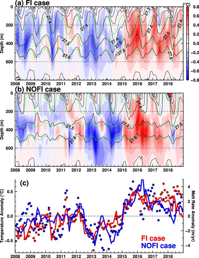
1698                                               K. Kusahara et al.: Ocean–cryosphere interactions in Lützow-Holm Bay

   More recently, several studies have started to focus on the    ter increase Ekman convergence (downwelling), thickening
Totten ice shelf, Wilkes Land, East Antarctica, as a newly        WW in the surface to subsurface layers and thinning a warm-
recognized hot spot of active ice shelf–ocean interaction         water layer below WW. Conversely, weaker winds in the
caused by a CDW intrusion (Rintoul et al., 2016; Silvano          summer season relax the Ekman convergence, leading to a
et al., 2016, 2018, 2019). Ice shelves in the Amundsen and        relatively thin WW layer and a thicker CDW layer in deep
Bellingshausen seas and the Totten ice shelf have a com-          layers.
mon feature: the Antarctic Circumpolar Current (ACC) is              Although multi-year fast ice usually covers the south-
proximal to the Antarctic continental shelf regions, and thus     ern part of LHB, the fast ice has experienced extensive
CDW can affect regional coastal water masses. The South-          breakup events with irregular intervals of a few decades
ern Ocean has three large-scale cyclonic (subpolar) gyres:        (Aoki, 2017; Ushio, 2006). A relatively large breakup oc-
the Ross, Kerguelen, and Weddell gyres (Gordon, 2008).            curred from March to April 2016. As a result of the breakup
Amundsen and Bellingshausen seas and the offshore region          event, the 58th JARE could perform an extensive campaign
of Wilkes Land correspond to southeastern sides of the Ross       of trans-bay ship-based hydrographic observations to investi-
and Kerguelen gyres, respectively, where the southward de-        gate possible ocean–ice shelf/glacier interaction in LHB (Hi-
flection of the large-scale ocean circulations brings warm wa-    rano et al., 2020). The in situ oceanographic observations
ter poleward to the Antarctic continental shelves (Armitage       in the bay elucidate intrusion of CDW onto the continental
et al., 2018; Dotto et al., 2018; Gille et al., 2016; McCart-     shelf, and the warm-water signal extends to the front of the
ney and Donohue, 2007; Mizobata et al., 2020). By anal-           SGT, indicating active ice–ocean interaction at the SGT.
ogy to the relationship between the southward deflection of          As mentioned above, LHB and the SGT appear to be a
the ocean circulations and the active ice shelf melting areas,    suitable place for examining Antarctic ocean–ice shelf in-
one can naturally speculate there is active ocean–ice shelf in-   teraction in the Atlantic sector. However, they have been
teraction around the southeastern side of the Weddell Gyre        overlooked until very recently. Although the recent oceano-
(Ryan et al., 2016). In fact, looking at an estimate of basal     graphic observations show the existence of CDW in the bay
melt rate from Rignot et al. (2013), a glacier tongue (Shi-       (Hirano et al., 2020), little is known about the variability in
rase Glacier tongue, SGT) exhibits a high basal melt rate         the warm water intrusions, and it is not clear how the intru-
of 7 ± 2 m yr−1 , although the areal extent is small. The up-     sion is controlled. As far as we know, there is no numeri-
stream glacier, Shirase Glacier in Lützow-Holm Bay (LHB),         cal modeling study that focuses on the water mass forma-
Enderby Land, East Antarctica, is one of the fastest laterally    tion/exchange and the ocean–ice shelf interaction in this re-
flowing glaciers around Antarctica (Nakamura et al., 2010;        gion. In this study, we perform a numerical simulation to il-
Rignot, 2002).                                                    lustrate coastal water masses and ocean–ice shelf interaction
   The coastal Japanese Antarctic station, Syowa Station,         in LHB. In particular, we focus on the seasonal–interannual
is located within LHB, and it is the main platform of the         variability in the warm water intrusion from shelf break to
Japanese Antarctic Research Expedition (JARE) for Japanese        the bay and basal melting at the SGT. Additionally, we in-
Antarctic sciences. LHB is bounded to the east by the north–      vestigate the roles of fast ice in ocean conditions and the ice–
south-oriented coastline and to the west by the northwest–        ocean interaction in this area.
southeast coastline/ice shelf (Fig. 1), and the semi-closed bay
is open to the north. As an interesting feature, LHB is usually
covered with multi-year fast ice throughout the year (Fraser
et al., 2012, 2020; Nihashi and Ohshima, 2015; Ushio, 2006).      2     Numerical model, bottom topography, and
The fast-ice cover has made in situ oceanographic observa-              atmospheric conditions
tions difficult. Notably, JARE (31st and 32nd expeditions
from 1990 to 1992) conducted year-round oceanographic             2.1    An ocean–sea ice–ice shelf model for Lützow-Holm
observations through drilled holes on the fast ice in LHB.               Bay
Ohshima et al. (1996) analyzed these observation data and in-
vestigated the seasonal cycle of Winter Water (WW), which         This study utilized a coupled ocean–sea ice–ice shelf model
is surface-to-subsurface cold water formed in a winter mixed      (Kusahara and Hasumi, 2013, 2014). The model employed
layer. Furthermore, they proposed a physical mechanism of         an orthogonal, curvilinear, horizontal coordinate system.
seasonal change in the WW thickness: the strength of the          Two singular points of the horizontal curvilinear coordinate
alongshore wind stress controls the WW thickness through          in the model were placed on the East Antarctic continent
Ekman convergence. At that time, although the study did not       (72◦ S, 30◦ E, and 69◦ S, 50◦ E) to regionally enhance the
focus on warm water near the bottom, their ocean observa-         horizontal resolution around the LHB region while keeping
tions in the bay clearly show the presence of CDW (char-          the model domain of the circumpolar Southern Ocean. An ar-
acterized by high temperatures > 0.0 ◦ C and high salinity        tificial northern boundary was placed at approximately 30◦ S.
> 34.5 psu) below WW (characterized by the near-surface           The same technique to enhance the regional horizontal reso-
freezing temperatures). Stronger winds in autumn and win-         lution has been used for several studies on Antarctic coastal

The Cryosphere, 15, 1697–1717, 2021                                                  https://doi.org/10.5194/tc-15-1697-2021
K. Kusahara et al.: Ocean–cryosphere interactions in Lützow-Holm Bay                                                               1699

Figure 1. Bottom topography and the draft of ice shelves/glaciers around the Lützow-Holm Bay (LHB) area. Dashed red contours indicate
the horizontal grid spacing in the model. Map inset shows our focal region in the Southern Ocean. Gray-shaded areas are fast-ice regions.
Background bottom topography is derived from the ETOPO1 dataset, and the local topography in the area enclosed with an orange box has
been replaced with the recently compiled dataset (Sect. 2.2 and Fig. 2a). SGT indicates the Shirase Glacier tongue; SkG indicates Skallen
Glacier; KG indicates Kaya Glacier. Major place names are shown in the inset: Weddell Sea (WS), Ross Sea (RS), Amundsen Sea (AS), and
Bellingshausen Sea (BS).

ocean modeling (Kusahara et al., 2010, 2017; Marsland et                  In the ice shelf component, we assumed a steady shape
al., 2004, 2007).                                                      in the horizontal and vertical directions. The freshwater
   The vertical coordinate system of the ocean model was               flux at the base of ice shelves was calculated with a three-
the z coordinate. There are four vertical levels of 5 m cell           equation scheme, based on a pressure-dependent freezing
thickness below the ocean surface and 49 levels of 20 m                point equation and conservation equations for heat and salin-
thickness in the depth range from 20 to 1000 m. Below this             ity (Hellmer and Olbers, 1989; Holland and Jenkins, 1999).
depth, the vertical spacing varies with depth (50 m thick-             We used the velocity-independent coefficients for the thermal
ness for 1000–2000 m, 100 m thickness for 2000–3000 m,                 and salinity exchange velocities (i.e., γt = 1.0 × 10⁻⁴ m s−1
and 200 m thickness for 3000–5000 m). The maximum ocean                and γs = 5.05 × 10⁻⁷ m s−1 ; Hellmer and Olbers, 1989),
depth in the model was set to 5000 m to save computational             although ocean velocity-dependent coefficients have often
resources. The model has an ice shelf component for the z-             been used in recent ice shelf–ocean modeling studies. Ve-
coordinate system (Losch, 2008). A partial step representa-            locity magnitudes under the ice shelves strongly depend on
tion was adopted for both the bottom topography and the ice            the horizontal and vertical grid resolutions (Gwyther et al.,
shelf draft to represent them optimally in the z-coordinate            2020), and thus we preferred using the velocity-independent
ocean model (Adcroft et al., 2002). The sea ice compo-                 version to minimize the dependency originated from the
nent used one-layer thermodynamics (Bitz and Lipscomb,                 model configuration. The modeled meltwater flux and the as-
1999) and a two-category ice thickness representation (Hi-             sociated heat flux were imposed on the ice shelf–ocean inter-
bler, 1979). Prognostic equations for the sea ice momentum,            face.
mass, and concentration (ice-covered area) were taken from                The horizontal grid spacing over the LHB region was less
Mellor and Kantha (1989). Internal ice stress was formulated           than 2.5 km (Fig. 1). This relatively high horizontal resolu-
by the elastic–viscous–plastic rheology (Hunke and Dukow-              tion enabled us to accurately reproduce the coastline, ice-
icz, 1997), and sea ice salinity was fixed at 5 psu. Unstable          front line, and bottom topography in the focal region. The
stratification produced in the ocean model was removed by              background bathymetry for the Southern Ocean in this model
a convective adjustment, and a surface mixed layer scheme              was derived from ETOPO1 (Amante and Eakins, 2009),
(Noh and Kim, 1999) was used for the open ocean, as in our             while the ice shelf draft and bathymetry under the ice shelf
previous study of a circumpolar Southern Ocean modeling                were obtained from the RTopo-2 dataset (Schaffer et al.,
that showed a reasonable representation of seasonal mixed              2016). The bottom topography in the LHB bay region (70–
layer depth over the Southern Ocean (Kusahara et al., 2017).           68◦ S, 35–40◦ E) was replaced with a detailed topography
                                                                       that blended multi-beam surveys from the 51st–55th JAREs;

https://doi.org/10.5194/tc-15-1697-2021                                                      The Cryosphere, 15, 1697–1717, 2021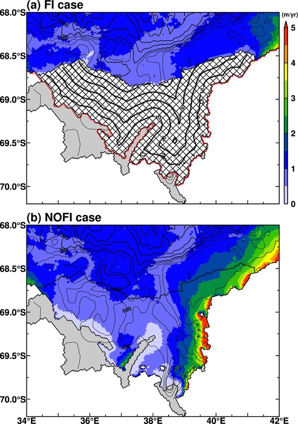
1700                                               K. Kusahara et al.: Ocean–cryosphere interactions in Lützow-Holm Bay

point echo sounding using sea ice drill holes from the 9th–        included in the first two experiments (CKDRF and FI cases)
22nd JAREs (Moriwaki and Yoshida, 1983); depth data from           but not in the NOFI case. In the CKDRF case, the model con-
the nautical chart created by the Japan Coast Guard (JCG), in      tinued to be driven by the year 2005 surface forcing to check
which ship-based single-beam echo sounding data obtained           a model drift in the experiments. In the FI and NOFI cases,
in several JAREs were included; and ETOPO1 (Amante and             a hindcast simulation was carried out for the period 2006–
Eakins, 2009). The detail for the compiled bottom topog-           2018 with interannually varying forcing. The difference be-
raphy was described in the “Methods” section in Hirano et          tween the FI and NOFI cases allows us to examine the role
al. (2020). In Sect. 2.2, we compare this recently compiled        of fast ice in the ocean and cryosphere components. It should
bottom topography with several topography datasets.                be noted that the two icescape configurations were largely
   As mentioned in the introduction, extensive fast ice has        simplified compared to the actual time-varying fast-ice dis-
been identified along the East Antarctic coast (Fraser et al.,     tribution. The numerical results from the two extreme cases
2012; Nihashi and Ohshima, 2015), and the existence of per-        were utilized to examine the transient response of the ocean
sistent fast ice characterizes LHB. We introduced areas of         and cryosphere components from the FI case to the NOFI
multi-year fast-ice cover into LHB in the model as constant-       case and the impact of the fast ice on the quasi-equilibrium
thickness (5 m) ice shelf grid cells. Although, in reality, the    state.
horizontal distribution and thickness of fast ice vary sea-           In the CKDRF and FI case, we used the same coeffi-
sonally and interannually (Aoki, 2017; Fraser et al., 2012;        cients of the ice shelf thermal and salinity exchange veloc-
Ushio, 2006), the spatial distribution of multi-year fast ice      ities, even for the fast-ice–ocean interaction. The coefficients
in the model was assumed to be constant in time as a first         of the exchange velocities were based on observational facts
approximation. This assumption is likely more valid here in        (Hellmer and Olbers, 1989), and the magnitude corresponds
LHB than in more dynamic areas of fast-ice cover, where            to an ocean velocity of 15–20 cm s−1 under ice shelves in
breakouts can occur many times per year. The fast ice in the       velocity-dependent parameterization (Holland and Jenkins,
model prohibited momentum, heat, and freshwater fluxes at          1999). Under the ice shelf, the velocity-independent param-
the ocean surface with the atmosphere. Since the fast ice in       eterization with the coefficients is partially justified with the
the model was treated as thin ice shelf, the fast ice also pro-    strong tidal flows as an unresolved process in the models
vided freshwater to the ocean surface, based on the melt rate      without tidal forcing. However, since fast ice is located in a
diagnosed with thermodynamic fast-ice–ocean interaction.           more open area, this parameterization is expected to overesti-
   The model’s initial conditions of temperature and salin-        mate the basal melting at fast ice. To investigate the sensitivi-
ity were derived from the Polar science center Hydrographic        ties of the fast-ice melting and the impact on ice shelf melting
Climatology (Steele et al., 2001), with zero ocean velocity        and environmental ocean conditions with respect to the ex-
over the model domain. Note that the water properties in           change coefficients, we conducted three additional sensitivity
the climatology over the Southern Ocean come from World            experiments with multiplying factors of 0.5, 0.2, and 0.0 on
Ocean Atlas 1998 (Conkright et al., 1999). North of 40◦ S,         the thermal and salinity exchange coefficients (FIMOD05,
ocean temperature and salinity were restored to the monthly        FIMOD02, and FIMOD00) only under the fast-ice region.
mean climatology throughout the water column with a damp-          In the FIMOD00 case, although there are no heat, salinity,
ing timescale of 10 d. Outside of the focal region where the       or freshwater exchanges between fast ice and the ocean, ice
horizontal resolution becomes coarser than 10 km, sea sur-         shelves (e.g., the SGT) can melt as in the baseline experi-
face salinity was restored to the monthly mean climatology         ments.
to suppress unrealistic deep convection in some regions (e.g.,
the Weddell Sea).                                                  2.2   Bottom topography in Lützow-Holm Bay
   Daily surface boundary conditions for the model were
surface winds, air temperature, specific humidity, down-           The accuracy of bottom topography is critically vital for
ward shortwave radiation, downward longwave radiation,             high-resolution ocean modeling because the geostrophic
and freshwater flux. To calculate the wind stress and sensi-       contour/bottom topography strongly controls ocean flows
ble and latent heat fluxes, we used the bulk formula of Kara       (including CDW intrusions on the East Antarctic continen-
et al. (2000). When the surface air temperature was below          tal shelf; e.g., Nitsche et al., 2017) and the associated water
0 ◦ C, precipitation was treated as snow. Daily reanalysis at-     properties. Several large-scale compilations of bottom topog-
mospheric conditions were calculated from the ERA-Interim          raphy are now available. As an example, Fig. 2b–f show spa-
dataset (Dee et al., 2011). The ocean–sea ice–ice shelf model      tial distributions of bottom topography in our focal region
was first integrated for 20 years with the year 2005 forcing       in five bottom-topography datasets: ETOPO1 (Amante and
for spin-up to obtain a quasi steady state in the ocean and        Eakins, 2009), ETOPO5 (NOAA, 1988), GEBCO (IOC, IHO
cryosphere components.                                             and BODC, 2003), RTopo-1 (Timmermann et al., 2010a),
   We performed three baseline experiments: CKDRF, FI,             and RTopo-2 (Schaffer et al., 2016). As can be seen in Fig. 2,
and NOFI cases. All three experiments started from the fi-         there are considerable differences in the representations of
nal state of the spin-up integration. The effect of fast ice was   bottom topography, in particular in the southern half of LHB

The Cryosphere, 15, 1697–1717, 2021                                                    https://doi.org/10.5194/tc-15-1697-2021
K. Kusahara et al.: Ocean–cryosphere interactions in Lützow-Holm Bay                                                                  1701

Figure 2. Comparison of water depth representation in the topographic datasets (a: this study; b: ETOPO1; c: ETOPO5; d: GEBCO;
e: RTopo-1; f: RTopo-2/IBCSO). The red lines in panels (b)–(f) indicate the grounding line in the model (a). Circles with color in panel (a)
are observed depth measurements from the point echo sounding using sea ice drill holes and the JCG nautical chart (subsampled to avoid
clutter in the panel). In panel (a), the two submarine canyons around the sill are labeled WC and EC, and four troughs extending southward
from the sill are marked T1, T2, T3, and T4 from west to east.

where fast ice is particularly present. All of the products have        them and extends toward the SGT. In the southern part of the
a sill-like feature at around 68.4◦ S, 37.0◦ E, and depression-         trough, there is a north–south elongated depression at the lat-
like features south of it. In the five products, ETOPO1 cap-            itudes from 69.5 to 70◦ S with a maximum depth of approxi-
tures the large-scale features when comparing with JARE’s               mately 1600 m. The feature is confirmed in the observational
in situ depth observations (see dots in Fig. 2a). For this rea-         data. We consider our dataset, in which available bathymet-
son, the ETOPO1 dataset was utilized for the background                 ric observations were taken into account, the best estimate of
topography for the recently compiled topography (Hirano et              bottom topography in the LHB region at this moment.
al., 2020).
   Looking at the recently compiled topography, there are               2.3    Atmospheric conditions
two submarine canyons on both sides of the sill at the lati-
tude of 68.4◦ S. It should be noted that the bathymetric fea-
                                                                        In this subsection, we show seasonal changes in the long-
tures around the sill, including the submarine canyons, are
                                                                        term-average fields of mean sea level pressure (MSLP) over
well constrained by the observed depths derived from the
                                                                        the Southern Ocean and surface winds off the LHB region
point echo sounding and the hydrographic chart (colored dots
                                                                        (Fig. 3), based on the ERA-Interim climatology for our main
in Fig. 2a). Acoustically observed data confirm that the sill
                                                                        analysis period 2008–2018. A circumpolar pattern of low
top is ∼ 500 m deep and surrounded by an at least ∼ 850 m
                                                                        pressure at high southern latitudes and high pressure at lower
deep western submarine canyon and a 1600 m deep eastern
                                                                        latitudes accompanies a prevailing westerly wind over the
submarine canyon. South of the sills, there is a large depres-
                                                                        Southern Ocean in the latitudes from 40 to 60◦ S, a pre-
sion whose maximum depth is deeper than 1000 m. From the
                                                                        dominant spatial pattern in the high-latitude Southern Hemi-
depression, four troughs extend southward. The most east-
                                                                        sphere. There are three regional minimums of the MSLP in
ern trough (labeled T4) is the longest and deepest among
                                                                        the Weddell Sea, the Indian sector, and the Amundsen Sea,

https://doi.org/10.5194/tc-15-1697-2021                                                        The Cryosphere, 15, 1697–1717, 2021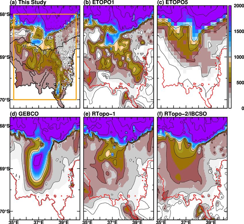
1702                                                   K. Kusahara et al.: Ocean–cryosphere interactions in Lützow-Holm Bay

                                                                        the fast ice in this model is represented as an uppermost one-
                                                                        grid ice shelf. Fast ice becomes a physical barrier between
                                                                        ocean and atmosphere, modifying the exchanges of surface
                                                                        heat, freshwater, and momentum fluxes. The southern half of
                                                                        LHB is usually covered with fast ice, except during breakup
                                                                        events. Before examining the effects of the fast-ice cover on
                                                                        the ocean conditions in LHB and the SGT melting in the next
                                                                        section, we show the difference in the surface forcing with
                                                                        and without fast-ice cover.
                                                                           Sea ice production is a key proxy for cold and saline water
                                                                        mass formation along the Antarctic coastal margins (Morales
                                                                        Maqueda et al., 2004; Tamura et al., 2008, 2016) because
                                                                        brine rejection (very high salinity water from sea ice to the
                                                                        ocean when sea ice is formed) is proportional to the sea ice
                                                                        production. The newly formed cold and saline water mass de-
                                                                        stratifies the local water columns over the Antarctic coastal
                                                                        regions. Perennial fast ice is a very effective thermal insulator
                                                                        between the atmosphere and ocean due to its thickness (NB
                                                                        a perfect insulator in the model, meaning no atmosphere/sea
                                                                        ice–ocean interaction). Therefore, we investigate the differ-
                                                                        ence in sea ice production in the FI and NOFI cases (Fig. 4).
                                                                        Of course, there is zero sea ice formation under the fast ice
Figure 3. Seasonal climatology of atmospheric circulation (a–d)         in the LHB region in the FI case (Fig. 4a). In the NOFI case,
over the Southern Ocean and (e–f) in the region off Lützow-Holm         areas of relatively high sea ice production are produced along
Bay. Color and vectors show the 3-month average of surface air          the eastern coastline in the bay (Fig. 4b). The sea ice produc-
pressure and 10 m wind fields, respectively. The climatology is cal-    tion in the NOFI case reaches a maximum in autumn (April–
culated from the ERA-Interim dataset for the period 2008–2018.          May), and the active sea ice production areas are confined to
The red box in the upper panels indicates the region for panels (e)–    the coastal regions within a 30 km distance of the coastline
(h). The area enclosed by the yellow line in the middle panels is       or the ice front (Fig. 5a). The difference in sea ice production
the area for averaging the 10 m wind for panel (i). In panel (i), the
                                                                        in the fast-ice region plays a major role in regulating the ver-
monthly climatologies of wind vector and wind speeds (black: ab-
                                                                        tical profile of the coastal water masses and the subsequent
solute speed; red: alongshore speed) are displayed. The red vector
is a unit vector of the defined alongshore direction.                   SGT basal melting, as shown later.
                                                                           Ocean melts the fast-ice base as well as ice shelves, and
                                                                        thus the fast-ice basal melting provides freshwater to the
and the regional minimums deepen in the autumn and winter               ocean surface. The basal melting depends on the magnitudes
seasons. South of the air pressure minimums (i.e., Antarctic            of the thermal and salinity exchange coefficients at the fast-
coastal regions) is a prevailing easterly wind regime, which            ice–ocean interface. The basal melt rate and amount of the
is the driving force of westward-flowing currents along the             fast ice and ice shelves/glaciers in the experiments are sum-
Antarctic coastal margins (Thompson et al., 2018).                      marized in Table 1. Here, we briefly comment on the feasi-
   LHB is located on the southeastern side of the low pres-             bility of the modeled basal melt rate at the fast ice and exam-
sure in the Weddell Sea (see the red box in Fig. 3). In the             ine the freshwater (meltwater) forcing under the fast ice in
longitude bands, the westerly wind blows north of 62◦ S, and            the experiments. The climatological average precipitation is
the easterly wind blows south of 64◦ S throughout the year              about 60 cm water equivalent per year (2008–2018 average in
(Fig. 3e–h). The alongshore component dominates the east-               the ERA-Interim dataset). This surface input is used here to
erly wind, and the wind speed reaches the maximum in au-                gauge the feasibility of the estimated magnitude of the fast-
tumn (from March to June) and the minimum in the spring                 ice basal melting in the model. The mean melt rate of the fast
and summer seasons (from October to January).                           ice in the FI case is estimated to be 2.29 m yr−1 , which can
                                                                        not be balanced by the local precipitation. With decreasing
                                                                        the magnitude of the exchange velocities in the FIMOD05
3   Difference in the surface forcing in the experiments                and FIMOD02 cases, the fast ice’s mean melt rates decline
    with and without fast-ice cover                                     to 1.50 and 0.83 m yr−1 , respectively. Taking account of the
                                                                        inputs from the dynamical interaction with drifting sea ice
Fast ice is formed by sea ice fastening to the Antarctic coast-         (Fraser et al., 2012; Massom et al., 2010) and the snow-ice
line and/or ice shelf front, and the typical thickness is a few         formation of the fast ice (Zhao et al., 2020), the melt rate
meters (Fraser et al., 2012; Giles et al., 2008). Note again that       in the FIMOD02 seems to be in a realistic range. The mod-

The Cryosphere, 15, 1697–1717, 2021                                                         https://doi.org/10.5194/tc-15-1697-2021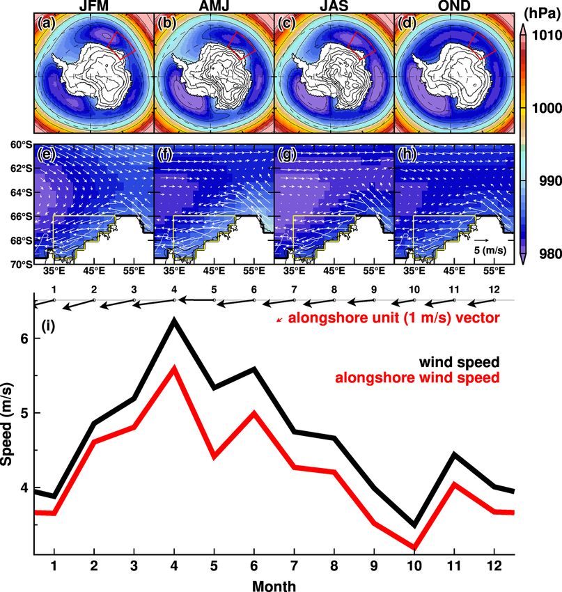
K. Kusahara et al.: Ocean–cryosphere interactions in Lützow-Holm Bay                                                                               1703

Table 1. Annual mean basal melt rate (m yr−1 ) and amount (Gt yr−1 ) at glaciers in the LHB and fast ice. SGT indicates the Shirase Glacier
tongue; SkG indicates Skallen Glacier; KG indicates Kaya Glacier.

                                                         SGT                        Fast ice                         SkG                           KG
               Area extent (km2 )                         559                    19.3 × 10³                          29.7                          703
               FI                   15.2 m yr−1 (7.8 Gt yr−1 )   2.29 m yr−1 (40.7 Gt yr−1 )   19.0 m yr−1 (0.52 Gt yr−1 )   11.8 m yr−1 (7.6 Gt yr−1 )
 Experiments

               FIMOD05              14.5 m yr−1 (7.5 Gt yr−1 )   1.50 m yr−1 (26.5 Gt yr−1 )   18.0 m yr−1 (0.49 Gt yr−1 )   11.1 m yr−1 (7.1 Gt yr−1 )
               FIMOD02              14.8 m yr−1 (7.6 Gt yr−1 )   0.83 m yr−1 (14.7 Gt yr−1 )   18.2 m yr−1 (0.50 Gt yr−1 )   11.0 m yr−1 (7.1 Gt yr−1 )
               FIMOD00              14.3 m yr−1 (7.3 Gt yr−1 )     0.0 m yr−1 (0.0 Gt yr−1 )   16.6 m yr−1 (0.45 Gt yr−1 )   10.0 m yr−1 (6.4 Gt yr−1 )
               NOFI                  8.8 m yr−1 (4.5 Gt yr−1 )               not applicable     7.5 m yr−1 (0.20 Gt yr−1 )    4.5 m yr−1 (2.9 Gt yr−1 )

                                                                                   Figure 5. Seasonal and interannual variations in sea ice production
                                                                                   in the LHB region in the NOFI case. Note that sea ice production
                                                                                   is calculated from sea ice freezing, not including sea ice melting. In
                                                                                   panel (a), the seasonality of the sea ice production was calculated in
                                                                                   10 km bins of the distance from the coastline/ice front (see contours
                                                                                   over the fast-ice region in Fig. 4a), and the gray boxes show the sea
                                                                                   ice production within 30 km of the coastline/ice front. The monthly
                                                                                   climatology is the average over the period 2008–2018.

Figure 4. Maps of annual sea ice production (m yr−1 ) in the (a) FI
                                                                                   ice–ocean velocity of 3–4 cm s−1 , which is roughly consis-
and (b) NOFI cases. The sea ice production was averaged over the
                                                                                   tent with the modeled ocean flow speed under the fast ice.
period 2008–2018. The meshed region in panel (a) indicates the
fast-ice cover. Gray-shaded areas show ice shelves/glaciers. The                      In this study, we use results from the FI case to represent
contours over the fast-ice cover in panel (a) represent the minimum                the baseline ocean–cryosphere conditions for the existence of
distance from the coastline or ice front (shown by red dots). The                  the fast ice, taking account of the continuity from the spin-
black contours show the water depth, with 200 m (1000 m) intervals                 up integration, although the basal melting at the fast ice is
in the regions shallower (deeper) than 1000 m.                                     exaggerated (Table 1). In the several following analyses and
                                                                                   figures, we show the results from the FIMOD series as well
                                                                                   as the baseline experiments to show the dependency of the
eled ocean velocities just under the fast ice vary from a few                      modeled ocean–cryosphere conditions on the different fast-
cm s−1 to 15 cm s−1 depending on the location and season,                          ice melting. As a result (shown later), the impacts of the fast-
with the approximate mean speed of 5 cm s−1 . The exchange                         ice meltwater on the ocean conditions and the SGT basal
coefficients in the FIMOD02 case correspond to the relative                        melting are much smaller than those of sea ice production

https://doi.org/10.5194/tc-15-1697-2021                                                                    The Cryosphere, 15, 1697–1717, 2021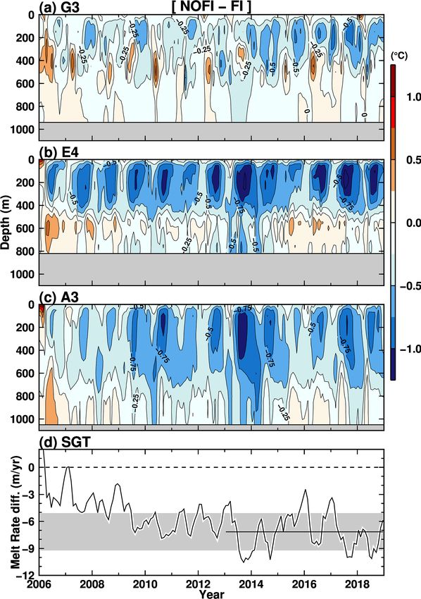
1704                                                  K. Kusahara et al.: Ocean–cryosphere interactions in Lützow-Holm Bay

                                                                      Figure 7. Seasonal variation in basal melt rate at the Shirase Glacier
                                                                      tongue. Black, blue, red, and green lines show results from the CK-
Figure 6. Time series of basal melt rate at the Shirase Glacier       DRF, NOFI, and FI cases and the ice-radar-derived estimate (au-
tongue (a: the full integration period of 33 years including peri-    tonomous phase-sensitive radio echo sounder – ApRES; Hirano et
ods of the initial 20-year spin-up and the CKDRF case; b: the last    al., 2020), respectively. Thick lines represent the mean melt rate av-
14 years corresponding to the period 2005–2018). In panel (b), red,   eraged over the whole of the SGT. Thin red and blue lines show the
blue, and black lines show the results from the FI, NOFI, and CK-     regional basal melt rate around the ApRES observation (see Fig. 8
DRF cases, respectively. Thin orange, yellow, and green lines are     for the locations). Shade or vertical bars indicate the standard devi-
the results from the FIMOD05, FIMOD02, and FIMOD00 cases,             ation of the monthly basal melt rate in the period 2008–2018, show-
respectively. The equivalent annual melt rate (m yr−1 ) is used for   ing the model’s inherent variability and interannual variability. The
the vertical scale.                                                   scale of the vertical axis is the equivalent annual melt rate (m yr−1 ).

difference in the experiments with and without the fast-ice           4.1   Transient response and quasi-equilibrium of the
cover.                                                                      CDW intrusion into LHB and the SGT melting

                                                                      The NOFI case corresponds to the sudden removal of all the
4   Warm water intrusion into LHB and active basal                    fast ice in LHB on 1 January 2006. The main difference in
    melting at the SGT                                                the model configuration between the FI and NOFI cases is
                                                                      the surface boundary conditions in the fast-ice-covered area,
Since the model started from a motionless state with the cli-
                                                                      as explained in the previous section. In this section, firstly,
matological ocean properties, it requires a spin-up time to ad-
                                                                      we compare the modeled ocean properties in both the FI
just simulated ocean circulation and water masses in LHB to
                                                                      and NOFI cases with the recent hydrographic observations
a quasi steady state. In this study, we can use the time series
                                                                      in LHB (Hirano et al., 2020). The in situ observations were
of the basal melt rate at the SGT to monitor the spin-up of the
                                                                      conducted in January 2017, which means 8–9 months after
ocean–cryosphere system in LHB (Fig. 6) because the basal
                                                                      the extensive fast-ice breakup in the austral autumn (March–
melting is an integrated result from the interaction between
                                                                      April) of 2016 (Aoki, 2017). The observations seem to have
the ocean flow and coastal water masses. As can be seen in
                                                                      been made in a transient phase following the large breakup
Fig. 6a, the basal melt rate reaches a quasi steady state after
                                                                      event. Using the time evolution of the differences in the
approximately 20 years. There is a slightly declining trend
                                                                      ocean properties and the SGT melting between the FI and
in the basal melt rate after the 20-year spin-up, due to an in-
                                                                      NOFI cases, we roughly estimate a transient timescale of the
herent model drift or insufficient spin-up for the circumpolar
                                                                      ocean–cryosphere system responding to the sudden fast-ice
Southern Ocean. However, the magnitude of the declining
                                                                      removal. Finally, after showing the transient timescale of a
trend of the melt rate in the CKDRF case is much smaller
                                                                      few years, we use monthly climatology for the ocean and
than interannual variability and the difference between the
                                                                      cryosphere components over the period 2008–2018 to exam-
FI and NOFI cases (Figs. 6b and 7). Therefore, we can use
                                                                      ine the difference in the quasi-equilibrium states in the FI and
the results from the two baseline experiments to examine the
                                                                      NOFI cases.
seasonal and interannual variability.

The Cryosphere, 15, 1697–1717, 2021                                                         https://doi.org/10.5194/tc-15-1697-2021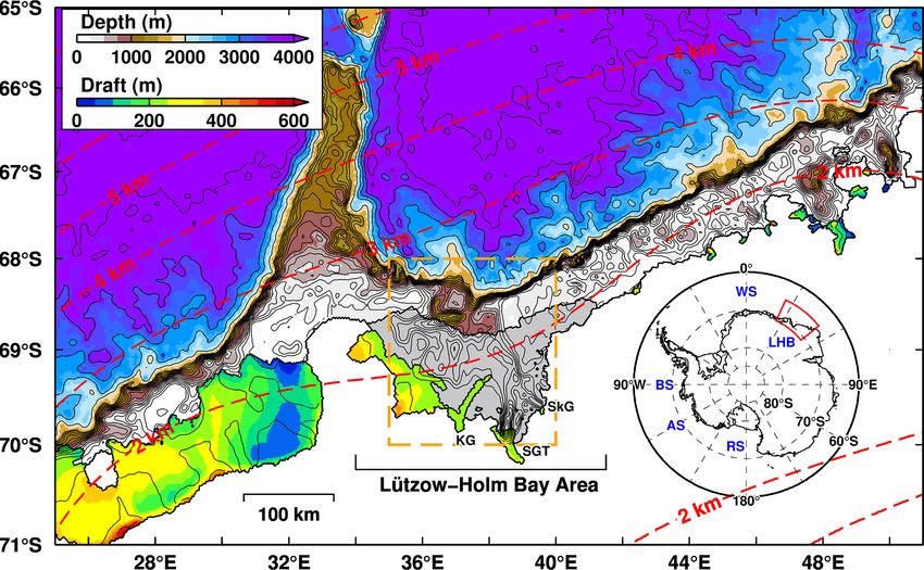
K. Kusahara et al.: Ocean–cryosphere interactions in Lützow-Holm Bay 1705
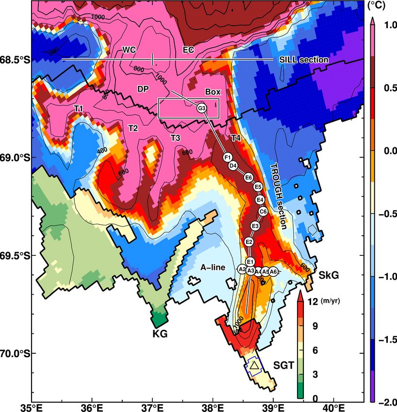
Figure 8. Key sections and observational stations used in this study.
Colors represent the modeled ocean bottom temperature in January
and the annual mean basal melt rate in the NOFI case. The variables
were averaged over the period 2008–2018. White circles with sta-
tion names show positions of the in situ oceanographic observations
for the comparisons in Figs. 9 and 11. Black lines connecting the ob-
servational stations are defined as the TROUGH section and A line.
The thick zigzag black lines are the grounding line, the ice-front
line, and the fast-ice edge in the FI case. The area enclosed with
the blue line on the SGT is the averaging area for calculating the
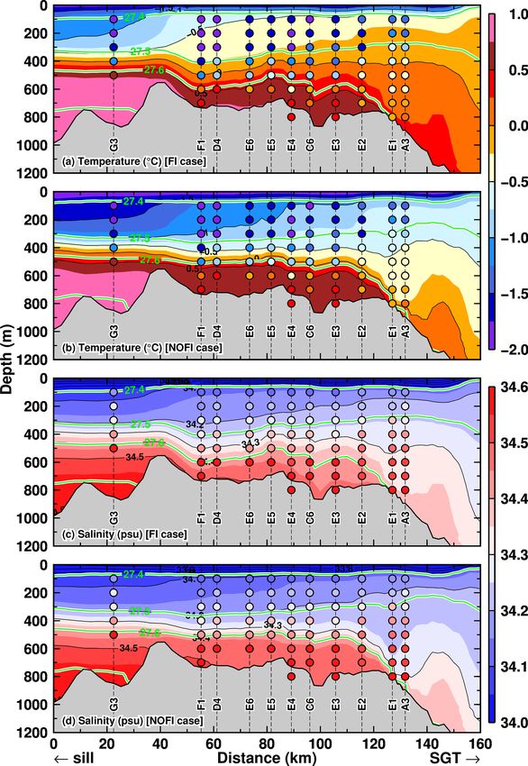
regional basal melt rate around the location of ApRES (triangle). Figure 9. Vertical profiles of (a, b) potential temperature and (c, d)
SGT indicates the Shirase Glacier tongue; SkG indicates Skallen salinity along the TROUGH section in January in the two cases
Glacier; KG indicates Kaya Glacier. WC and EC refer to the west- (a and c for the FI case, b and d for the NOFI case). Green curves
ern and eastern submarine canyons, respectively. T1, T2, T3, and T4 indicate the contours of potential density anomalies. The model’s
refer to the troughs in the LHB. Sill sections near the shelf break are variables were averaged over the period 2008–2018. The horizontal
used to show vertical profiles in Fig. 9. A box is used for averaging axis indicates the distance from the starting point of the TROUGH
ocean properties in Figs. 12 and 20. section located near the deepest depression in LHB (see the line of
the TROUGH section in Fig. 8). Circles filled with the color on ver-
tical dashed lines indicate the observed ocean properties in January
and February 2016 (Hirano et al., 2020).
Figure 8 shows key sections and the observational stations
used in this study, with the spatial distributions of the mod-
eled bottom temperature in January and the annual mean
basal melt rate at the ice shelves/glaciers. The TROUGH Fig. 9 are subsampled ocean properties from the in situ ob-
section is a north–south-running observational line from the servations (Hirano et al., 2020). The two-layer feature in the
deep depression to the SGT ice front, and the A line is located model is consistent with the observation results. In particular,
at approximately 69.58◦ S. Warm water intrusions into LHB the model can reasonably represent the temperature of the
from the shelf break are clearly seen in Fig. 8 (for the NOFI inflowing warm water in the bottom layer along the trough
case), and the warmest waters are identified along the four (Fig. 9a and b). The temperature of the warm water intru-
troughs (T1, T2, T3, and T4 from west to east). Warm water sion is much warmer than the local freezing point and thus
in the trough T4 (e.g., along the TROUGH section) extends a driver of high basal melting at the SGT. The warm water
southward toward the SGT and Skallen Glacier (SkG). intrusion in the FI case (Fig. 9a) is thicker than in the NOFI
In both the FI and NOFI cases, the vertical profiles of the case (Fig. 9b), and the temperature difference between the
ocean properties along the TROUGH section have a clear two cases becomes the largest in a subsurface–intermediate
two-layer structure consisting of a cold fresh surface layer depth range (50–400 m). The observed ocean temperature in
and a warm saline deep layer (Fig. 9). Colored circles in the subsurface–intermediate depths is colder than −1.0 ◦ C,
https://doi.org/10.5194/tc-15-1697-2021 The Cryosphere, 15, 1697–1717, 2021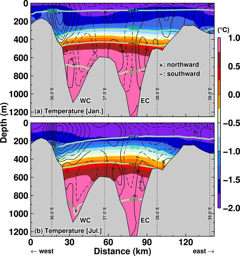
1706                                                K. Kusahara et al.: Ocean–cryosphere interactions in Lützow-Holm Bay

indicating that the temperature profile in the observation is
more similar to that in the NOFI case. The existence of the
relatively cold water in the upper layers suggests that the wa-
ter in LHB has experienced surface cooling after the fast-ice
breakup. Looking at the salinity profiles, again, the model
represents the clear intrusion of the high-salinity signal along
the bottom from the sill to the SGT (Fig. 9c and d). There are
some model biases in salinity. The observed salinity near the
bottom throughout the section is higher than in the model by
more than 0.1 psu. Since the less saline signal in the model is
found near the sill region, the salinity biases probably come
from an insufficient representation of salinity values in the
continental-slope and continental-rise regions. Even taking
into account the salinity bias throughout the section, the near-
bottom salinity at the southernmost stations (E1 and A3) is
substantially underestimated in both cases, in particular in
the NOFI case. The near-bottom salinity in the FI case is
higher than in the NOFI case, and thus the FI case appears to
better represent the near-bottom water salinity at the south-
ernmost stations. The better agreement of the bottom salinity
between the observation and FI case suggests that the near-
bottom signal responds more slowly to the fast-ice breakup
and that the in situ observations within 1 year of the breakup
event captured the transitions of the coastal water masses.
   Next, we try to estimate a transition timescale of the
ocean–cryosphere system in LHB from the breakup to fast-
ice-free conditions, using time evolution of deviations of the
model results in the NOFI case from those in the FI case
(NOFI − FI). Figure 10 shows the time evolution of the ocean
temperature difference at stations G3, E4, and A4 along the         Figure 10. Time evolutions of the differences (NOFI − FI) in ocean
TROUGH section (Figs. 8 and 9) and the SGT basal melt               temperature at the stations G3, E4, and A3 on the TROUGH section
rate. Just after removing the fast ice (i.e., 2006 in the NOFI      (Figs. 8 and 9), and the SGT basal melting. The black line and shade
case), the surface layers are warmed up (clearly seen at sta-       in panel (d) indicate the average of the SGT melt rate difference
                                                                    averaged over the period 2013–2018 between the FI and NOFI cases
tions E4 and A3), exposing the ocean surface to a warm at-
                                                                    and the standard deviation.
mosphere and downward shortwave radiation in summer. In
the subsequent winter, the ocean experiences a substantial
cooling from the surface to intermediate depths due to sea ice      from the NOFI case for the comparison along the A line.
formation in the bay (Fig. 4b). The difference in the tempera-      The vertical section of potential temperature along the A line
ture profile appears to be stable within a few years of remov-      with the normal velocity (positive for northward) illustrates
ing the fast ice. This is also confirmed in the difference in the   that the warm water intrusion is strongly trapped near the bot-
SGT basal melt rate (Fig. 10d). The basal melt rate rapidly         tom on the eastern flank of the deep trough (Fig. 11). In Jan-
decreases by approximately 4 m yr−1 in the first winter, and        uary, the warm water (> 0 ◦ C) is present in the bottom layer
then it continues to decline for a few years. Comparing with        denser than 27.6 kg m−3 and the magnitude of the southward
the melt rate difference in the last 6 years when the equilib-      flow is larger than 10 cm s−1 (Fig. 11a). On the western side
riums are assumed to be reached in the FI and NOFI cases            of the trough, the northward flow of cold and fresh water is
(black line and gray shade in Fig. 10d showing the mean and         reproduced at the surface and intermediate depths. The over-
the standard deviations of the melt rate difference between         turning circulation in the model is generally consistent with
the two cases), the melt rate deviation is in the standard de-      that inferred from the observed water properties (tempera-
viation range after a few years.                                    ture; salinity; oxygen; and the stable oxygen isotope ratio,
   At the end of this subsection, we compare the ocean tem-         δ 18 O; Hirano et al., 2020). These patterns of the ocean prop-
perature profile along the A line of the observations and that      erties and circulation are persistent throughout the year but
of the NOFI case (Fig. 11). As shown above, the observations        with a smaller magnitude of the warm water intrusion in au-
seem to capture the transient conditions. Since the observed        tumn and winter (Fig. 11b).
temperature profile along the TROUGH section is more sim-
ilar to that in the NOFI case (Fig. 9), here we use the results

The Cryosphere, 15, 1697–1717, 2021                                                      https://doi.org/10.5194/tc-15-1697-2021
K. Kusahara et al.: Ocean–cryosphere interactions in Lützow-Holm Bay 1707
Figure 11. Vertical profiles of potential temperature along the A line
in (a) January and (b) July in the NOFI case, with the velocity nor-
mal to the section (cm s−1 ). Positive velocity indicates northward
flow. Green curves indicate the contours of potential density anoma-
lies. The model’s variables were averaged over the period 2008–
2018. The horizontal axis indicates the distance from the starting
point of the A-line section (see the line of the A line in Fig. 8). Cir- Figure 12. Seasonal variation in potential temperature (color) and
cles filled with the color in panel (a) indicate the observed ocean potential density anomaly (green contours) averaged over the box
properties in January and February 2016 (Hirano et al., 2020). area (Fig. 8) in the (a) FI and (b) NOFI cases. The variables were
averaged over the period 2008–2018.
4.2 Seasonal changes in Ekman downwelling and
density surfaces box area is explained by the seasonality of the alongshore
wind stress (Fig. 2). Figure 13 shows a seasonal cycle of the
Ohshima et al. (1996) pointed out that the seasonal change monthly Ekman downwelling calculated from the alongshore
in the alongshore wind controls the seasonality of the sur- wind stress. Here, the Ekman upwelling–downwelling veloc-
face WW thickness in LHB (i.e., thickening in autumn and ity (negative values for downwelling) was calculated by τ
winter and thinning in spring and summer). A recent observa- (ρf 1L)−1 , where τ is alongshore (southwestward; see the
tional study by Hirano et al. (2020) indicated the weakening unit vector in Fig. 3i) wind stress (but ignoring the existence
of the alongshore wind in summer allows the thickening of of sea ice in this calculation), ρ is ocean density, f is the
CDW in the bay. Here, to confirm the wind-driven ocean pro- Coriolis parameter at 68.5◦ S, 1L is the assumed horizontal
cesses, we examine the seasonality in ocean density surfaces scale of the downwelling. We used 1L = 25 km for the cal-
and temperature in the deep depression of the bay. A control culation, and the width is approximately 3-fold the internal
box was defined just south of the sill on the shelf break to Rossby radius (8 km). We admit that the choice of 1L is arbi-
estimate the seasonal cycle of ocean temperature and density trary, but the calculated Ekman downwelling can reasonably
profiles (Fig. 12). The box encompasses the observation sta- explain the seasonality of the density surfaces, particularly
tion G3 (Fig. 8). As shown in the previous figures (Figs. 9 in the FI case. The seasonal cycle in the FI case is more ap-
and 11), there is relatively warm water in the deep layer be- parent than that in the NOFI case because the fast-ice cover
low the cold surface layer. The two-layer structure persists plays a role as a physical barrier for the surface momentum
throughout the year in the mouth of the bay. The potential flux, and the wind stress curl input caused by the combination
density surfaces of 27.5 and 27.6 kg m−3 fluctuate at approx- of the fast-ice edge and the alongshore easterly wind results
imately 400 and 500 m depths, respectively, with a shoaling in pronounced Ekman downwelling in this region (Ohshima,
in summer and a deepening in autumn and winter. The sea- 2000).
sonal differences in the density surfaces are up to 100 m. As
suggested in the literature (Hirano et al., 2020; Ohshima et
al., 1996), this seasonal cycle of the density surfaces in the
https://doi.org/10.5194/tc-15-1697-2021 The Cryosphere, 15, 1697–1717, 20211708 K. Kusahara et al.: Ocean–cryosphere interactions in Lützow-Holm Bay 4.3 Basal melting at the SGT The warm water intrusion along the eastern flank of the deep trough (Figs. 9 and 11) results in a high basal melt rate at the SGT (Table 1 and Figs. 6 and 7). As an exam- ple, looking at the SGT melt rate distribution in the NOFI case (Fig. 8), active basal melting with the annual melt rate higher than 10 m yr−1 is represented in the northern part of the SGT, where the warm water contacts first the SGT base. The southern part also has a high basal melt at approximately 5 m yr−1 . Since the circumpolar-averaged basal melt rate of the Antarctic ice shelves was estimated to be in a range from Figure 13. Seasonal variations in monthly Ekman downwelling (a 0.81 to 0.94 m yr−1 (Depoorter et al., 2013; Rignot et al., product of Ekman velocity and a month (30 d)). The monthly value 2013), we can conclude that the SGT is a hot spot of ocean– is climatology averaged over the period 2008–2018. ice shelf/glacier interaction caused by the CDW intrusions across the shelf break (Table 1). Next, we examine the relationship of the seasonal cycles Hirano et al. (2020) used an ice radar of an autonomous between the water mass transport into the SGT cavity and the phase-sensitive radio echo sounder (ApRES) to estimate monthly basal melt rate at the SGT in the FI and NOFI cases basal melt rate at the SGT for the period from February 2018 (Fig. 14). We calculated the inflow transport of water masses to January 2019 (green line in Fig. 7). Here, we briefly com- exactly across the SGT ice front and the mean temperature pare the seasonality of the SGT basal melt rates of the model in potential density bins with an interval of 0.02 kg m−3 . In result and of the observation-based estimate. The model and both cases, relatively warm water with temperatures higher observation both show a high basal melting rate in summer than −0.5 ◦ C is present in the denser classes throughout the and a relatively low melt rate in autumn and winter (Fig. 7). year, and the transport of the warm waters into the cavity The SGT average basal melt rates in the model show a rapid reaches a maximum in summer (from November to Febru- increase from September to December, consistent with the ary), resulting in the high basal melt rate at the SGT. There ApRES estimate. These general agreements provide some are differences in the temperature and the total inflow volume confidence in the model results in this study, especially for of the warm water into the cavity in the two cases. The tem- the seasonality of the SGT basal melt rate. It should be noted perature of the inflow in the FI case is higher than that in the that the ApRES was located on the high-gradient zone of the NOFI case, mainly because sea ice production in the south- basal melt rate in the model (Fig. 8) and the observation pe- ern part of LHB (i.e., the fast-ice cover region in the FI case) riod was less than 1 year. When comparing the local basal in the NOFI case leads to cooling of the surface–intermediate melt rates of the model and observation, the model underes- waters, particularly in autumn and winter (Figs. 4, 5, and 14). timates the seasonal amplitude of the basal melt rate. This While the total transport of the inflow in the FI case is rela- indicates the model underestimates the seasonal cycle of the tively stable throughout the year, there is a substantial sea- warm-water inflow into the cavity under the ApRES position. sonal cycle of the total inflow transport in the NOFI case. In- The bottom topography under the SGT is outside of our com- tegrated effects of the surface fluxes over the southern LHB piled topography data, and thus it was not well constrained region (e.g., sea ice production and wind stress on the ocean by the observed topography. The uncertainty in the bottom surface) that are missing in the FI case are likely to cause topography probably leads to the discrepancy in the seasonal the pronounced seasonal cycle of the total inflow transport. amplitude of the local basal melt rate. In both cases, the temperature of the inflowing water masses As shown in Sect. 3, a series of numerical experiments starts to decrease in March (and the total inflow volume trans- with different exchange coefficients under the fast ice shows port declines in autumn and winter in the NOFI case), lead- different meltwater flux from the fast-ice base (Table 1), and ing to a rapid decrease in ocean heat flux into the SGT cav- results from these experiments allow us to examine the im- ity. Consistent with the seasonal cycle of the warm water in- pact of the fast-ice melting on the SGT basal melting. The trusion, the SGT shows a substantial seasonal variation in difference in the SGT melting among the experiments with the basal melt rate from 12 m yr−1 in winter to 18 m yr−1 in the fast-ice cover (FI and FIMOD series) is much smaller summer in the FI case and 6 m yr−1 in winter to 13 m yr−1 in than that between the FI and NOFI cases. This is because the summer in the NOFI case (Fig. 7). It should be noted again buoyant meltwater from the fast ice mainly affects the surface that the melt rate in winter, even in the NOFI case, is still water, and the SGT draft is deeper than the depth of the mod- much higher than the circumpolar-averaged basal melt rate. ified surface water. This explanation also holds for neighbor- The high basal melt rate throughout the year is caused by the ing glaciers, the Skallen and Kaya glaciers (Table 1). persistent warm water intrusion in the deep layer in the LHB region. The Cryosphere, 15, 1697–1717, 2021 https://doi.org/10.5194/tc-15-1697-2021
K. Kusahara et al.: Ocean–cryosphere interactions in Lützow-Holm Bay 1709
Figure 14. Seasonal variation in water mass transport flowing into
the SGT cavity (mSv, left axis for boxes) with the potential tem-
Figure 15. Vertical profiles of potential temperature along the sill
perature in potential density anomaly bins of 0.02 kg m−3 (color)
section (at 68.5◦ S) in (a) January and (b) July in the NOFI case,
and the mean basal melt rate (m yr−1 , right axis for black lines) in
with the velocity normal to the section (cm s−1 ). Positive veloc-
the (a) FI and (b) NOFI cases. Green dots and yellow squares rep-
ity indicates northward flow. Green curves indicate the contours of
resent boundaries of 27.5 and 27.4 kg m−3 of the potential density
potential density anomalies. The model’s variables were averaged
anomaly, respectively. The variables were averaged over the period
over the period 2008–2018. The horizontal axis indicates the dis-
2008–2018.
tance from the western side starting point of the sill section (see the
line of the sill section in Fig. 8).
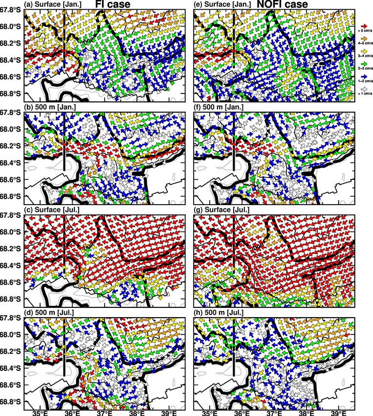
4.4 Warm water intrusions from the continental shelf
break and slope regions into LHB
of less dense cold water on the western flank of the WC
The previous analyses in this section demonstrated that the (Fig. 15) and surface-intensified southward flow over the
warm water intrusions onto the continental shelf predomi- eastern flank of the EC in winter (Fig. 15b). The surface-
nate the ocean structure in LHB (Figs. 8, 9, and 11), the water intensified southward flow brings a large volume of cold
masses flowing into the SGT cavity (Fig. 14), and the mag- water into the bay in winter, in particular through the EC
nitude of the SGT basal melting (Figs. 6 and 7). Here, we (Fig. 16b and d).
examine in detail water mass exchanges across the sill sec- Next, we show the spatial distribution of ocean flows at
tion through the submarine canyons and ocean flow on the the surface and 500 m depth to identify the origin of the warm
upper continental-slope regions. water mass flowing into LHB through the submarine canyons
Firstly, we show vertical profiles of the potential tempera- (Fig. 17). Southwestward flows along the continental slope
ture, potential density, and north–south ocean flow along the predominate surface flows throughout the year. This along-
sill section at the latitude of 68.5◦ S to identify locations of shore surface flow is strong in winter and weak in summer
the warm water intrusions from the offshore region into LHB (panels a, c, e, and g in Fig. 17), which corresponds to the
(Fig. 15 for the NOFI case) and show the seasonal varia- seasonality of surface wind magnitude in this region (Fig. 3i).
tion in the southward inflow transport across the sill section Ocean flow patterns at 500 m depth are quite different from
in the FI and NOFI cases (Fig. 16). There are two subma- the surface flow patterns. In summer, a strong eastward flow
rine canyons in the section (we call the western and east- is produced on the continental slope between the 500 and
ern canyons WC and EC, respectively). Looking at the deep 2000 m isobaths. In this study, we use the term “undercur-
layers denser than 27.5 kg m−3 (Fig. 15), southward flows rent” to point out the eastward flow below the westward sur-
are present in the two submarine canyons and bring very face flow. Although the eastward undercurrent is found in
warm water (up to 1 ◦ C) into LHB. The southward flows both the FI and NOFI cases, the undercurrent in the FI case
of the deep warm waters (σ0 > 27.5 kg m−3 ; green squares is more vigorous than in the NOFI case. A part of the un-
in Fig. 16 showing the density boundary) are identified in dercurrent is redirected southward at the submarine canyons.
the two canyons throughout the year in both cases (Fig. 16). The southward flow brings warm water in the deep layer into
Looking at the upper layers, there is a strong northward flow LHB (Fig. 17b; see also Figs. 15a and 12). The southward
https://doi.org/10.5194/tc-15-1697-2021 The Cryosphere, 15, 1697–1717, 2021You can also read