A discrete interaction numerical model for coagulation and fragmentation of marine detritic particulate matter (Coagfrag v.1) - GMD
←
→
Page content transcription
If your browser does not render page correctly, please read the page content below
Geosci. Model Dev., 14, 4535–4554, 2021
https://doi.org/10.5194/gmd-14-4535-2021
© Author(s) 2021. This work is distributed under
the Creative Commons Attribution 4.0 License.

A discrete interaction numerical model for coagulation and
fragmentation of marine detritic particulate matter (Coagfrag v.1)
Gwenaëlle Gremion1 , Louis-Philippe Nadeau1 , Christiane Dufresne1 , Irene R. Schloss2,3,4 , Philippe Archambault5 ,
and Dany Dumont1
1 Institut des sciences de la mer de Rimouski, UQAR, Québec-Océan, Rimouski, Canada
2 Instituto Antártico Argentino, Buenos Aires, Argentina
3 Centro Austral de Investigaciones Científicas (CADIC-CONICET), Ushuaia, Argentina
4 Instituto de Ciencias Polares y Ambientales, Universidad Nacional de Tierra del Fuego, Ushuaia, Argentina
5 ArcticNet, Québec-Océan, Université Laval, Quebec, Canada

Correspondence: Gwenaëlle Gremion (gwenaelle.gremion@gmail.com) and Louis-Philippe Nadeau
(louis-philippe_nadeau@uqar.ca)

Received: 13 December 2020 – Discussion started: 15 January 2021
Revised: 9 May 2021 – Accepted: 18 May 2021 – Published: 23 July 2021

Abstract. A simplified model, representing the dynamics of         spectrum is then presented and shows significant improve-
marine organic particles in a given size range experiencing        ment in reducing the observed biases.
coagulation and fragmentation reactions, is developed. The
framework is based on a discrete size spectrum on which re-
actions act to exchange properties between different particle
sizes. The reactions are prescribed according to triplet inter-    1   Introduction
actions. Coagulation combines two particle sizes to yield a
third one, while fragmentation breaks a given particle size        The biological carbon pump is responsible for a significant
into two (i.e. the inverse of the coagulation reaction). The       fraction of the organic carbon exports from the surface to
complete set of reactions is given by all the permutations         the deep ocean (Passow and Carlson, 2012; Le Moigne,
of two particle sizes associated with a third one. Since, by       2019), thereby influencing the climate (Kiørboe and Thyge-
design, some reactions yield particle sizes that are outside       sen, 2001). Questions regarding the quantification and pre-
the resolved size range of the spectrum, a closure is devel-       diction of its efficiency and response times are still broadly
oped to take into account this unresolved range and satisfy        unanswered. The carbon pump yields a wide variety of pro-
global constraints such as mass conservation. In order to min-     cesses, involving the co-action of a large number of physi-
imize the number of tracers required to apply this model to        cal, chemical and biological variables (Denman et al., 2007).
an ocean general circulation model, focus is placed on the         Coupled ocean general circulation models (OGCMs) and
robustness of the model to the particle size resolution. Thus,     biogeochemical models (BGCs) contribute to our under-
numerical experiments were designed to study the depen-            standing of the relative importance of these processes. They
dence of the results on (i) the number of particle size bins       were developed for decades to assess the biological pump dy-
used to discretize a given size range (i.e. the resolution) and    namics at the global scale (e.g. Palmer and Totterdell, 2001;
(ii) the type of discretization (i.e. linear vs. nonlinear). The   Aumont et al., 2003; Dutkiewicz et al., 2005) or for specific
results demonstrate that in a linearly size-discretized config-    regions of the world (e.g. Sarmiento et al., 1993; Blackford
uration, the model is independent of the resolution. However,      and Radford, 1995; Doney et al., 2002; Wiggert et al., 2006;
important biases are observed in a nonlinear discretization. A     Karakaş et al., 2009).
first attempt to mitigate the effect of nonlinearity of the size      Since the pioneering work of Riley (1946), BGCs have
                                                                   been widely used in oceanography and their complexity
                                                                   never ceased to increase (Vichi et al., 2007; Anderson

Published by Copernicus Publications on behalf of the European Geosciences Union.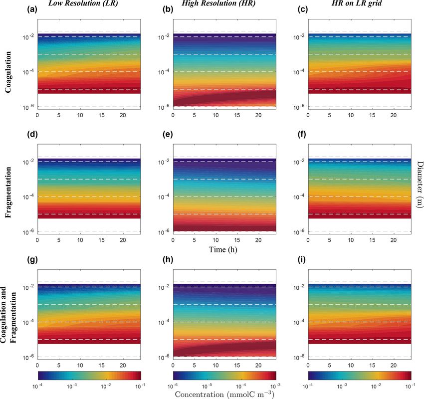
4536                        G. Gremion et al.: A discrete interaction numerical model for coagulation and fragmentation

and Gentleman, 2012). As reported by Leles et al. (2016),          count for processes by which the size, and consequently
they evolved from a nutrient–phytoplankton–zooplankton–            the settling velocities of these particles, can be altered with
detritus (NPZD) type (e.g. Palmer and Totterdell, 2001),           depth. Indeed, parameterization is generally achieved by con-
where multiple species and types of organic and inor-              straining detritus state variables by constant parameters or
ganic constituents of the pelagic system are gathered into a       depth-dependant functions (Gloege et al., 2017, e.g. expo-
broadly defined trophic compartment (Doney et al., 2003),          nential decay, Martin’s curve, ballast hypothesis) to repre-
to food webs of multiple plankton functional types (PFTs)          sent the actions of these processes and associated living or-
(Hood et al., 2006; Anderson et al., 2010). In most coupled        ganisms. As an example, coagulation (i.e. the formation of
OGCMs-BGCs, efforts have concentrated on achieving an              larger particles from the collision and aggregation of smaller
accurate representation of primary- and secondary-producer-        particles) increases particle size and may end up in aggregate
related particle dynamics, while the detritic compartment is       formation. Fragmentation is the opposite process, breaking
generally reduced to just one variable. The detritus particles     particles into smaller pieces. Both processes are then affect-
found in the ocean are nevertheless essential in the downward      ing particle size distribution but are barely explicitly imple-
export of carbon (Hill, 1992; Kriest, 2002). Considering only      mented or parameterized in OGCMs-BGCs.
one detritus variable may lead to important biases in car-            It is indeed based on the seminal work of Gelbard et al.
bon flux estimations. The size diversity of marine particles is    (1980) on the sectional representation of aerosol size distri-
wide, ranging from large, rapidly sinking particulate material     bution evolution due to collision and coagulation events, that
(i.e. marine snow) to small suspended particles and relatively     the first coagulation models applied to marine snow emerged.
non-labile dissolved organic matter (i.e. colloids), which usu-    Jackson and Burd (1998) extended the model of Gelbard
ally also show the highest abundances. Then, their represen-       et al. (1980) and applied it to the marine environment, point-
tation through a unique variable and mean values of its de-        ing out the role of fragmentation to counterbalance the im-
scriptive parameters such as sinking velocity (Doney et al.,       portance of coagulation (Jackson et al., 1995; Hill, 1996).
1996; Lima et al., 2002; Aumont et al., 2003; Dutkiewicz           We note that coagulation and fragmentation of particles is a
et al., 2005; Kishi et al., 2007) to cover the entire size range   natural phenomenon that happens in a very broad variety of
in BGCs is questionable.                                           situations. It has been studied in many disciplinary fields, in-
   To overcome this caveat and improve carbon export as-           cluding atmospheric sciences, especially in microdroplet and
sessments, the number of detritus-related variables in BGC         cluster formation (e.g. Pruppacher and Klett, 2010), but also
models can be increased to better represent the diversity          in chemistry (e.g. Lee et al., 2018), astrophysics and engi-
of the sinking particulate matter. For example, some stud-         neering (see the review of Pego, 2007). In oceanography, it
ies such as Moore et al. (2002); Wiggert et al. (2006); Yool       is also applied to aggregation of nanoplastics with colloids
et al. (2011); Butenschön et al. (2016); Kearney et al. (2020)     (Oriekhova and Stoll, 2018) or the oil–marine snow interac-
defined multiple (two or more) detritic compartments, each         tion (Dissanayake et al., 2018; Burd et al., 2020). We note
being connected differently with other variables and having        also that there a variety of modelling approaches, includ-
constant settling velocities. This approach can certainly in-      ing Lagrangian formulations with stochastic processes (e.g.
crease the level of realism, as these parameterizations are        Jokulsdottir and Archer, 2016). However, Eulerian formula-
made based on field or experimental evidence (Doney et al.,        tions are those that are still best applicable to OGCMs-BGCs
2003), but we see two major problems with them. First, the         and that will be considered more specifically here.
description in the numerical framework of a high number of            The present work stems from numerous Eulerian mod-
state variables enhances BGC models’ complexity and aug-           elling studies, most of which are listed by De La Rocha and
ments the number of parameters required to characterize re-        Passow (2007) and Jackson and Burd (2015) (e.g. for co-
lations among those variables (Denman, 2003). Ultimately,          agulation, refer to Jackson, 1990; Kriest and Evans, 1999;
it makes it challenging to properly couple them to OGCMs.          Jackson, 2001; Kriest, 2002, and for fragmentation to All-
In atmospheric microphysical modelling, where size spectral        dredge et al., 1990; Dilling and Alldredge, 2000; Kiørboe,
frameworks are used to represent the formation of clouds,          2000; Ploug and Grossart, 2000; Goldthwait et al., 2004;
efforts are made to use a small number of variables in 3-D         Stemmann et al., 2004) but these models are scarcely cou-
simulations to prevent a drastic increase of the computational     pled to OGCMs. It is probably due to the remaining quantita-
costs, to the expense of accuracy (Khain et al., 2015). The de-    tive unknowns regarding the ensemble of processes affecting
sire to improve realism and accuracy by adding complexity          transport efficiency of the particulate organic matter to depth
needs to be tempered by our ability to parameterize key pro-       by constraining particle size distribution even after decades
cesses as a compromise regarding computational costs and           of extensive work (Le Quéré et al., 2005; De La Rocha and
efficiency (Raick et al., 2006). As underlined by Anderson         Passow, 2007). The intrinsic heterogeneous nature of these
(2005), the conception of meaningful state variables and con-      processes at all spatiotemporal scales increases the challenge
stants in numerical models is crucial, and determining repre-      to properly implement them in complex OGCMs-BGCs and
sentative values for parameters can be challenging (Flynn,         to evaluate and predict the ocean’s role in the Earth’s carbon
2005; Le Quéré, 2006). Second, this approach does not ac-          budget. Similar challenges arise in atmospheric GCMs. Ac-

Geosci. Model Dev., 14, 4535–4554, 2021                                            https://doi.org/10.5194/gmd-14-4535-2021
G. Gremion et al.: A discrete interaction numerical model for coagulation and fragmentation                                 4537

cording to Kang et al. (2019), GCMs with full cloud micro-         or volume). To transpose the variables from the continuous
physics are still at an early stage in terms of understanding      form (Eq. 1) to a discrete form, Ls must be discretized in
and simulating many observed aspects of weather and cli-           size bins p such that
mate, and research is needed to circumvent these difficulties.
                                                                          N
   In order to circumvent the issues related to the representa-           X
                                                                   Ls =         1sp ,                                         (2)
tion of the dynamics of the complete particles size spectrum
                                                                          p=1
for OGCMs, we develop in this study a new numerical frame-
work where a particle’s size range is discretized in size bins,                   Rs
                                                                   where 1sp = spp+1 ds is the size range of the bin p, and the
and where concentration dynamics over these bins is driven
                                                                   terms (sp , sp+1 ) indicate the lower and upper size bounds of
by coagulation and fragmentation reactions. This framework
                                                                   this bin. Therefore, the particle content of a given bin p can
is designed to conserve mass over the size range and reac-
                                                                   be interpreted as its mean value
tions, and can accommodate size and mass linear and nonlin-
ear discretizations. Our approach differs from the so-called                      sZp+1
sectional approach of Jackson and Burd (2015) in that the                1
                                                                   Np =                 N ds   p = 1, . . ., N.               (3)
discretized size spectrum we use is an integral quantity that           1sp
                                                                                  sp
depends on the discretization, as opposed to a spectral den-
sity.                                                                 Note that other particle properties (e.g. diameter, volume,
   Since the main motivation for developing such a model is        density) are similarly interpreted as a bin-averaged value. For
to provide a tool allowing to characterize detritic variables      example, the particle diameterR corresponding to a given bin
relations and dynamics in coupled OGCMs without unrea-                                               s
                                                                   can be defined by Dp = 1s1 p spp+1 Dds. This diameter can
sonably increasing the computational cost, a formulation is
                                                                   in turn be used to determine the particle volume using an
sought that will attenuate the dependence of the results to the
                                                                   allometric relationship such as Vp = λ1 Dpλ2 (Jackson et al.,
size discretization resolution. Numerical experiments are de-
                                                                   1997; Li et al., 1998; Zahnow et al., 2011)1 . Using this bin-
signed to study the dependence of the results on (i) the num-
                                                                   averaged volume (Vp ), the particle content can be redefined
ber of size bins used to discretize a given size range (i.e. the
                                                                   as
resolution) and (ii) the type of discretization (i.e. linear vs.
nonlinear). Innovations of the approach with regard to previ-      Np = λ3 Vpλ4 ,                                             (4)
ously developed coagulation–fragmentation models and de-
signed detritic state variables are briefly discussed as well as   where λ3 and λ4 are parameters empirically determined
the potential for further improvements to allow the inclusion      through field and laboratory experiments depending on the
of the presented model into OGCMs to better estimate cur-          element chosen (Alldredge, 1998; see Table 1).
rent carbon export.                                                   The discrete form of Eq. (1) thus becomes
   The outline of the paper is as follows. Section 2 presents
the model description, Sect. 3 describes numerical experi-         Cp (t) = np (t)Np        p = 1, . . ., N,                  (5)
ments, and Sect. 4 presents and briefly discusses the results.
A summary of our main conclusions is given in Sect. 5.             where np is the particle number concentration in p (i.e. the
                                                                   number of particles in p), and N the total number of resolved
                                                                   size bin. In a closed system without sources and sinks of par-
                                                                   ticles, the total concentration, CT = N
                                                                                                         P
2     Model description                                                                                    p=1 p , is required to
                                                                                                               C
                                                                   be conserved over time. The time evolution of the concentra-
2.1    Discrete size spectrum                                      tion inside a given bin obeys the simple differential form

Whereas most laboratory and field studies estimate particle        dCp
                                                                       = Rp        p = 1, . . ., N,                           (6)
number concentration, n (m−3 ), along a size spectrum (Mc-          dt
Cave, 1984; Jackson et al., 1995), OGCMs use tracers’ (or el-
                                                                   where Rp represents all reactions occurring in p.
ements’) concentration, C (mmol m−3 ) (e.g. carbon or nitro-
gen), to study fluxes among the model compartments (Doney          2.2    Reaction for a triplet of particles
et al., 1996). These two variables are linked by
                                                                   Coagulation and fragmentation are, by essence, reactions that
C(t) = n(t)N ,                                              (1)    involve three particles. Coagulation involves two particles,
                                                                   with indices i and j , that collide and stick together to form
where N is the particles’ content of the chosen currency
                                                                   a third, larger one with index k. Conversely, fragmentation
(mmol).
   Considering a closed system in a given water volume with           1 The two constants parameters λ and λ depend on particles
                                                                                                       1    2
no particle sources or sinks, particles may be sorted over a       and can be obtain from laboratory experiments (Jackson et al.,
size range Ls with s a chosen size property (e.g. diameter         1997) or set by the user (Table 1).

https://doi.org/10.5194/gmd-14-4535-2021                                                  Geosci. Model Dev., 14, 4535–4554, 2021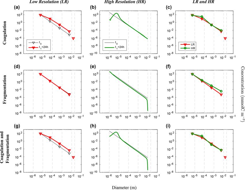
4538                           G. Gremion et al.: A discrete interaction numerical model for coagulation and fragmentation

Figure 1. Schematic representation of coagulation K and fragmentation F reactions between triplets of particles in a linear size discretization.
Coagulation is the process by which two particles with indices i and j collide and stick together to form a third, larger one with index k.
Fragmentation is the opposite process by which a particle k breaks into two smaller ones i and j . Size bounds are shown by vertical dashed
grey lines. Reactions involving two small particles (a) from the same size bin (i = j ) and (b) from two different size bins (i 6 = j ) are shown.

can be considered as the opposite reaction where a particle                   k is a triplet operator that represents both coagulation and
                                                                           δCi,j
k breaks into two smaller ones i and j , in line with what                 fragmentation reactions acting on a given bin:
was observed by Alldredge et al. (1990) in laboratory exper-
iments. Reactions involving more than three particles can al-                k       k         1
                                                                           δCi,j = δCi,j =        − Kij ni nj Ni + Fij nk Nk
ways be decomposed as a sequence of triplet reactions. Note                                    2
that i and j can originate from identical or different size bins.                      k       1
                                                                           δCjk ,i = δCj,i   =    − Kij ni nj Nj + Fij nk Nk .                (9)
In a linear size discretization, by definition, the k index al-                                2   |    {z     }   | {z }
ways refers to a particle belonging to a different bin than                                             Coagulation       Fragmentation
particles i and j . Then, the volume Vk of particle k result-
ing from the coagulation of particles i and j = 1. . .k obeys                 A bold index indicates the bin on which the reaction ap-
                                                                           plies (see also Fig. 2 for a visual explanation of this conven-
                                                                           tion). By construction, of the total number of k particles in-
                                                                           volved in the reaction in Eq. (8), half of this number is associ-
Vi + Vj = Vk      Vi ≤ Vj < Vk .                                  (7)      ated with i and the other half with j (Fig. 2), which explains
                                                                           why we multiply all the terms in Eq. (9) by 1/2. K is the
                                                                           coagulation rate, while F is the fragmentation rate. Coagu-
   The reaction is arbitrarily built so that the ith particle is al-       lation has been studied extensively in previous works both
ways the smallest one. From this assumption, the coagulation               in atmospheric (Pruppacher and Klett, 2010) and oceano-
reaction can be written as Vi +Vj ⇒ Vk , while fragmentation               graphic contexts (Jackson, 2001). It may be decomposed in
is Vk ⇒ Vi + Vj (Fig. 1). However, in the case of a nonlin-                a combination of a sticking probability and three main colli-
ear size discretization, this rule might be violated and this              sion mechanisms (Kiørboe et al., 1990; Ackleh, 1997; Engel,
situation is discussed in Sect. 2.6.                                       2000; Jackson, 2001): Brownian motion, fluid velocity shear
   In this model, the rules described above for particles will             and differential settling. Fragmentation (F) can be driven by
be applied on the bins’ discrete spectrum of Eq. (5). For ex-              biology, e.g. related to zooplankton activities such as graz-
ample, in a coagulation reaction implying a given triplet of               ing (Banse, 1990; Green and Dagg, 1997), and swimming
bins (i, j, k), the rate of change of the concentration in i will          behaviour (Dilling and Alldredge, 2000; Stemmann et al.,
depend on that of j , and they will conjointly prescribe the               2000; Goldthwait et al., 2004), or driven by physics, e.g.
rate of change of k. Such a reaction for a triplet of bins can             scales of turbulence (Alldredge et al., 1990; Kobayashi et al.,
be interpreted as multiple reactions for triplets of particles             1999).
that can be found in their respective bins (i, j, k). For a reac-
                                                                           2.3    Reaction matrices
tion implying a given triplet of bins (i, j, k), the evolution of
the concentration in each bin is described by the following                Let us now consider a set of discrete bins (p) that are linearly
set of differential equations:                                             incremented and have indices (i, j ) running from 1 to N. By
                                                                           construction, this yields reactions for k ranging from k = 2 to
                                                                           2N (i.e. 1+1 to N +N ). To account for the concentration evo-
dCi           dCj             dCk                                          lution associated with all possible reactions, we define four
        k                              k       k
    = δCi,j ;     = δCjk ,i ;     = −δCi,j − δCj,i .              (8)                                                   k ) defined earlier,
                                                                           matrices built from the triplet operator (δCi,j
 dt            dt              dt

Geosci. Model Dev., 14, 4535–4554, 2021                                                       https://doi.org/10.5194/gmd-14-4535-2021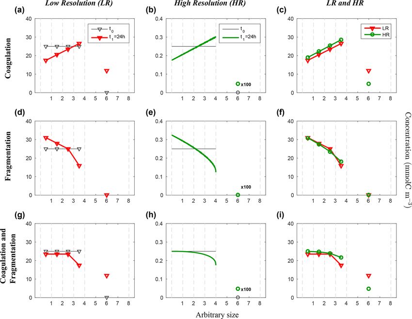
G. Gremion et al.: A discrete interaction numerical model for coagulation and fragmentation 4539
Table 1. Model variables and parameters.
Symbol Description Values Units
C Carbon concentration – mmol C m−3
n Particle number concentration Table 2 (particle) m−3
N Particle carbon content Table 2 mmol C
D Particle equivalent spherical diameter – m
V Particle volume – m3
R Reaction term – mmol C m−3 s−1
Ls Size range (i.e. diameter or volume) – m or m3
p Size bin index – –
N Total number of resolved size bin (i.e. resolution) Table 2 –
λ1 Coefficient for diameter to volume relation 2.8 –
λ2 Exponent for diameter to volume relation 2.49[a] –
λ3 Coefficient for volume to carbon content relation 1.09[b] -
λ4 Exponent for volume to carbon content relation 0.52[b] –
λ5 Coefficient for the resolution dependency function 0.99 –
λ6 Exponent the resolution dependency function −0.011 –
K Coagulation rate Table 2 m3 s−1
F Fragmentation rate Table 2 s−1
1t Time step Table 2 s
CT Total initial concentration 100 mmol C m−3
9 Slope of the size distribution −3[c] –
[a] Jackson et al. (1997). [b] Alldredge (1998). [c] Li et al. (2004); McCave (1984).
Di=j , Bi,j , Tj ,i and Fi,k , referring to diagonal, bottom, top The fourth matrix contains all the reactions acting on k,
and final matrices, respectively. which has dimensions N × 2N, and is given by
Matrix Di=j has dimensions N × N and accounts for re-
Fi,k [N × 2N] =
actions in which the two particles have the same size (i = j )
0 0 0 0 ··· 0
(Fig. 2a and c):
2δC1,1 2 0 0 0 ··· 0
δC 3 3
2
δC1,1 0 ··· 0
1,2 δC 2,1 0 0 ··· 0
0 4 δC 4 2δC2,2 4 4
δC3,1 0 ··· 0
δC2,2 ··· 0
1,3
Di=j [N × N] = .
.. .. .. .
(10) .. .. .. .. .. ..
.. . . . . . .
. . .
N
2N δC1,N−1 δC2,N−2 N N
δC3,N−3 N
δC4,N−4 ··· 0
0 0 ··· δCN,N
.
N +1 N +1 N +1 N +1 N +1
δC1,N δC2,N−1 δC3,N−2 δC4,N−3 ··· δCN,1
The square brackets above indicate the matrix dimensions.
0 N +2 N +2 N +2 N +2
δC2,N δC3,N−1 δC4,N−2 ··· δCN,2
Matrix Bi,j accounts instead for all reactions acting on i only
0 N +3 N +3 N +3
0 δC3,N δC4,N−1 ··· δCN,3
(where i < j , Fig. 2b and d): 0
0 0 N +4
δC4,N ··· N +4
δCN,4
.. .. .. .. ..
..
0 0 ··· 0 .
. . . . .
3 0 0 0 0 2N
2δCN,N
δC1,2 0 ··· 0 ···
Bi,j [N × N] = .. , (11)
.. .. .. (13)
. . . .
N+1 N +2
δC1,N δC2,N ··· 0 In F, the double line separates the resolved size range
(above) from the unresolved one (below). The latter con-
while Tj ,i accounts for those acting on j only (where j > i, tains reactions involving particle sizes outside the resolved
Fig. 2b and d): size range of the spectrum (i.e. reactions for which k > N ).
3 N+1 The unresolved range
0 δC2,1 ··· δCN,1
N+2
0 0 ··· δCN,2
Tj ,i [N × N ] =
.
(12) Solution strategies to parameterize reactions in the unre-
.. .. .. ..
. . . . solved range must obey two basic rules: (i) they must con-
0 0 ··· 0 serve the total concentration (CT ) in absence of external
https://doi.org/10.5194/gmd-14-4535-2021 Geosci. Model Dev., 14, 4535–4554, 2021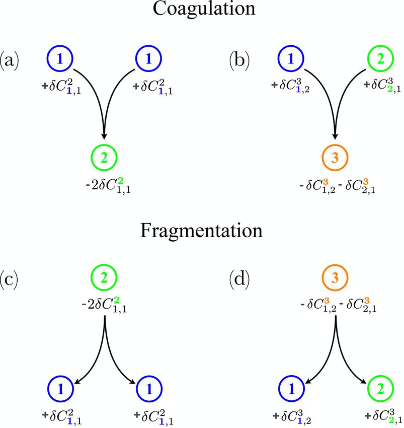
4540 G. Gremion et al.: A discrete interaction numerical model for coagulation and fragmentation
((Tj ,i + Dj =i ) + (Bi,j + Di=j ))[N × N + 1] =
3
2 3 N
2δC1,1 δC2,1 · · · δCN2 ,1
3
δC 3 4 2 N
1,2 2δC2,2 · · · δCN ,2
. .. ..
..
.
. . . .
,
(14)
3N 3 3
2N 2N
δC 2
1,N δC2,N · · · 2δCN ,N
0 0 ··· 0
Fi,k [N × N + 1] =
0 0 0 ··· 0
1C 2 0 0 ··· 0
1,1
Figure 2. Examples of individual reactions for a triplet of bins: 1C 3
3
1,2 1C2,1 0 ··· 0
(a, b) for coagulation only, assuming F = 0 and (c, d) for fragmen-
,
tation only, assuming K = 0 in Eq. (9). Panels on the left (a, c) in- .. .. .. .. ..
.
. . . .
volve terms of the diagonal matrix Di=j (Eq. 10), while panels on
the right (b, d) involve terms of the off-diagonal matrices B (Eq. 11) 1C N N
1C2,N −2 N
1C3,N ··· 0
1,N −1 −3
and T (Eq. 12) in Sect. 2.3. Different colours (blue, green and black)
3 3 3 3
represent different size bins. 2N 2N 2N 2N
PN PN PN
1C1,N j =N−1 1C2,j j =N −2 1C3,j ··· j =1 1CN,j
(15)
sources and sinks of particles and (ii) they must limit the un-
bounded growth of the particle size due to coagulation. Here where 1C = 2δC when i = j and δC otherwise, and K = 0
we propose a simple closure to account for the reactions in in 1C for k = 32 N. Equation (14) includes all reactions act-
this range. In order to comply with conservation of the to- ing on either i or j , while Eq. (15) includes all reactions act-
tal concentration in the size range (Ls ), at least one new bin ing on k. Since the unresolved range only involves reactions
must be added in which concentration fluxes in and out of acting on k, all the terms below the double line in Eq. (14) are
the resolved range are stored. Moreover, in order to avoid set to zero. Moreover, each term of the last row in Eq. (15)
unbounded growth of the size range due to coagulation, this can be viewed as a sum over all the elements of a given col-
extra bin must not be allowed to further coagulate with it- umn below the double line in Eq. (13). Note that, for sim-
self or any of the other particles sizes. As such, all reactions plicity, we choose to add only one extra bin in the unresolved
that fall into the unresolved range will be accounted for in a range, but one could alternatively choose to add up to N bins
single additional bin for which coagulation is prohibited but in order to improve this parametrization.
fragmentation back into the resolved range is allowed. This
extra bin can thus be interpreted as an average of all the re- 2.4 Summary of all reactions
actions in the unresolved range (N < k ≤ 2N ) and will be
referred to as k = 32 N. Applying this to Eqs. (10)–(13) yields Based on the matrices (Eqs. 14 and 15) and specific reaction
matrices with dimensions [N × N + 1]: rules previously described, the reaction vector Rp , represent-
ing all the reactions for a given bin (1 < p < N + 1) is given
by
Rp = Tj ,p + Dj =p · U + Bi,p + Di=p · U − Fi,p · U
= Xp + Yp − Zp
| {z } | {z }
− Coag + Frag + Coag − Frag
(16)
Geosci. Model Dev., 14, 4535–4554, 2021 https://doi.org/10.5194/gmd-14-4535-2021
G. Gremion et al.: A discrete interaction numerical model for coagulation and fragmentation 4541
where U is a unit vector with dimension [N], 2.5 Robustness to resolution
1
.. For a discrete representation of the full size range, Ls , larger
U = . . (17)
values of N imply higher resolution of the size spectrum.
1 The total number of reactions of the system described above
Coag and Frag in Eq. (16) are used to explicitly show the increases with the size of the reaction matrices, N (N + 1),
sign of the coagulation and fragmentation reactions from which is nearly a quadratic function of resolution. On the
Eq. (9). In other words, coagulation is removing concentra- other hand, coagulation and fragmentation are, respectively,
tion from p in Xp + Yp , while adding concentration to p in quadratic and linear functions of concentration, as shown in
Zp (and conversely for fragmentation). Equation (16) can be Eq. (9). Since concentration is itself a quantity that depends
rewritten as a sum of the following series: on resolution (Eq. 5), an asymmetric response between co-
agulation and fragmentation to changes in resolution is ex-
(p=1) : pected.
2
XN j +1 In order to build an intuition on the effect of resolution on
X1 = δC1,1 ; Y1 = δC1,j ; Z1 = 0
j =1 the reactions, consider a conservative system with a given
(1 < p ≤ N) : total concentration, CT = N
P
C
p=1 p , and a linear size dis-
Xp XN Xp−1
Xp =
p+i
δCp,i ; Yp =
p+j
δCp,j ; Zp =
p
1Ci,p−i cretization such that both the particle content and concen-
i=1 j =p i=1
tration are constants given by Np = 1 and Cp = CT /N, re-
3 spectively. To further simplify, assume that the rates of coag-
(p = N) :
2 ulation and fragmentation are constants given by K and F,
3
X2N XN N
Xp = 0; Yp = 0; Zp = 2
1Ci,j −i
respectively. For a conservative
P system, the sum of all reac-
j =N+1 i=j −N
tions integrates to zero, i.e. N+1
p=1 Rp = 0, such that CT re-
(18)
mains constant at all time. Since the sum of all reactions does
where 1C = 2δC when p = 2i and δC otherwise. An exam- not allow to keep track of the total concentration exchanged
ple of a complete set of reactions with N = 4 and its addi- along the spectrum, we instead define from Eq. (16) the total
tional bin 32 N = 6 is shown in Fig. 3. reaction amplitude as
Focusing on the resolved range only, Eqs. (16) and (18)
can be combined to yield a discrete version of the general- XN +1 XN +1
ized Smoluchowski equation (e.g. von Smoluchowski, 1916; RT = p=1 Xp + Yp = Z
p=1 p
Hansen, 2018): !
K CT 2
1 CT
XN p+i
Xp−1 p = N (N + 1) − +F ,
Rp = 1Cp,i − 1Ci,p−i 2 N N N
i=1 i=1
XN 1
=− i=1 2
(1 + δip ) Kip ni np Np − Fip ni+p Np
and since N = 1,
Xp−1 1
+ i=1 2
(1 + δ ip ) Kip ni n p−i Np − F ip n i+p−1 Np ,
(19) N +1 K 2 F
RT = − C + (N + 1) CT , (21)
N 2 T {z 2 }
where δip is the Kronecker delta function that is equal to 1 | {z } |
Coagulation Fragmentation
for i = p and zero otherwise. Notice that the above equation
gives the rate of change of concentration, whereas the tradi-
tional formulation for the Smoluchowski equation is written where the first term on the right-hand side is the total coag-
in terms of the number of particles. Equation (19) can thus ulation amplitude and the second term is the total fragmen-
be reformulated in terms of the number of particles as tation amplitude. In this simple example, dependenceto res-
N
X olution is revealed through the respective prefactors NN+1
δnp = − Kij ni np − Fip ni+p and (N + 1). It thus becomes obvious that fragmentation is
i=1
more sensitive to resolution than coagulation. This result can
p−1 be explained a posteriori if we notice that the total number
1X
+ Kij ni np−i − Fip ni+p−1 . (20) of reactions is nearly quadratic with N, while the coagula-
2 i=1
tion concentration is proportional to N −2 , cancelling most of
The factor of 1/2 in the second term ensures that the com- the variation with N. In contrast, the fragmentation concen-
bination of two particles yields a single larger particle. This tration is proportional to N −1 , which yields a larger resid-
is in contrast to the concentration, for which the combination ual dependence on N. To counterbalance this dependence on
is additive (see Eq. 8). resolution, the reaction terms are divided by their respective
https://doi.org/10.5194/gmd-14-4535-2021 Geosci. Model Dev., 14, 4535–4554, 2021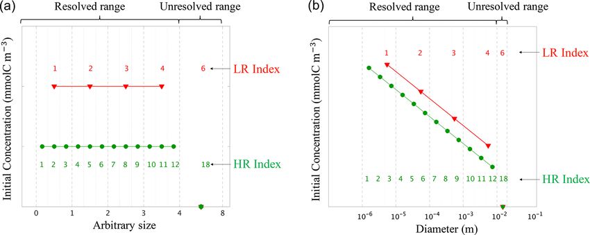
4542                                 G. Gremion et al.: A discrete interaction numerical model for coagulation and fragmentation

Figure 3. Example of a complete set of reactions applied to N = 4 size bins, with an additional class 32 N = 6. Concentration evolution
vectors are shown on top with the four size bins defined by the size range, and the last one representing the size bin 32 N . Bottom matrices
are modified versions of (a) T + B + 2D (Eq. 14) and (b) F (Eq. 15). Coloured areas and arrows indicate an exchange with the concentration
vector. Solid and dashed arrows indicate coagulation and fragmentation reactions, respectively.

resolution-dependent coefficients such that                                        does not imply however that mass conservation is necessar-
                                                                               ily violated. Consider, for example, a simple nonlinear dis-
                    1         N                            1
  k
δCi,j     k
      = δCi,j =          −           Kij ni nj Ni   +            Fij nk Nk         cretization where bins are each separated by an order of mag-
                    2        N +1                         N +1
                                                                               nitude (1, 10, 100 µm3 , etc.). Coagulation of particles belong-
                    1         N                             1
                                                                                   ing to bins 1 and 10 µm3 would ideally produce a particle

            k
δCjk ,i = δCj,i   =      −          Kij ni nj Nj    +            Fij nk Nk .
                    2        N +1                         N +1
                       |          {z            }     |       {z         }         size of 11 µm3 . However, since 11 µm3 is much closer to bin
                               Coagulation                  Fragmentation
                                                                                   10 µm3 than bin 100 µm3 (the next larger bin), all the concen-
                                                                            (22)   tration associated with this reaction will fall into the 10 µm3
   While the general case with non-constant contents and                           bin, thus violating volume conservation, yet conserving the
concentrations yields a similar qualitative dependence on N,                       concentration associated with the reaction. We thus modify
this simple parametrization produces significant biases in the                     Eq. (7) to allow that the resulting size of a coagulation reac-
nonlinear experiment (E2) described in the Sect. 4.2. Thus, a                      tion is not required to be strictly equal to the sum of the two
more exhaustive study on robustness to resolution is needed                        reacting particles (and conversely for fragmentation), i.e.
in order to improve this parametrization, and solutions strate-
gies are discussed in Sect. 4.3.
                                                                                   Vi + Vj ≤ Vi+j .                                           (23)
2.6    Nonlinear size spectrum

For simplicity, we chose to describe the above framework                              The main consequence of Eq. (23) is that it modifies the
using a linear size discretization (i.e. where bins are equally                    reaction matrices (Eqs. 14 and 15). In Eq. (14), only the
distributed along the size range). However, this choice was                        k indices will be modified by a nonlinear discretization. In
arbitrary and we now generalize the framework to a non-                            Eq. (15), the elements themselves will be redistributed on
linear size discretization, which is a more natural choice for                     different rows of the matrix. For a logarithmic discretization
representing marine particles. A nonlinear size discretization                     that enhances resolution towards smaller particles, elements
can be seen as local variations of the resolution in the full                      will be moved upwards in the F matrix as an increased num-
size range. For example, for a given total number of bins,                         ber of reactions yield Vi + Vj 6 = Vi+j . For example, δC1,2  3

N, switching from a linear to a logarithmic spacing increases                      could be switched from the third row using a linear spec-
resolution for the small particles, while decreasing it for the                    trum to δC1,22 in the second row using a logarithmic spec-

large particles. Intuitively, this choice seems better suited to                   trum. Conversely, elements will be moved downwards in the
represent marine particles that have a wider variety of micro-                     F matrix if a discretization that enhances resolution towards
scopic than macroscopic particles.                                                 larger particles is chosen. Here, we do not explicitly write the
   In this context, the main difference with the framework                         matrix encompassing all possible cases since this would be
described in the previous sections is that volume conserva-                        unnecessarily complex. The construction of the reaction ma-
tion can be violated when using a nonlinear size spectrum;                         trices (Eqs. 14 and 15) is done numerically at the beginning
i.e. Eq. (7) is no longer valid. Although counterintuitive, this                   of our algorithm (see Gremion and Nadeau, 2021).

Geosci. Model Dev., 14, 4535–4554, 2021                                                               https://doi.org/10.5194/gmd-14-4535-2021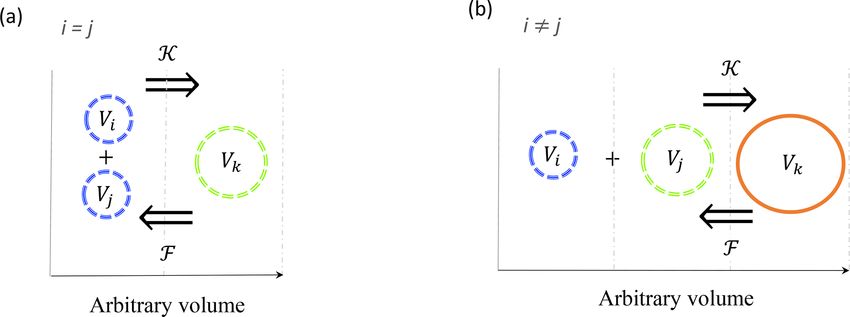
G. Gremion et al.: A discrete interaction numerical model for coagulation and fragmentation 4543
2.7 Application to a plankton ecosystem model value of 23 N is added to represent the unresolved size range,
which increases the total number of bins to N = 401 and
The framework presented here gives rise to N variables N = 5, respectively. For each resolution, three simulations
that together represent detritic particulate matter. Like other are performed: two simulations where coagulation (K) and
variables of plankton ecosystem models, these additional fragmentation (F) are considered separately, and one simula-
variables must be treated as Eulerian tracers submitted tion where they are combined (KF). In total, 12 simulations
to diffusive and advective transport. In a typical three- are performed with parameter values summarized in Tables 1
dimensional OGCM, the evolution of the carbon concentra- and 2.
tion Cp (mmol C m−3 ) belonging to the size bin p is given
by
3.1 Initialization
∂Cp ∂Cp
= − ∇ · uCp + ∇ · K∇Cp − wp + Sp
∂t ∂z For each configurations, all experiments are initialized from a
− Lp + Rp , (24) reference distribution at very high resolution (i.e. N † = 4000
bins) that is meant to represent an ideal distribution. This
where u = ı̂u + ˆv + k̂w is the velocity field and ∇ = ı̂ ∂x∂
+ discretization is indicated by the symbol †. The total carbon
∂ ∂ concentration is set to CT = 100 mmol C m−3 , and initial con-
ˆ ∂y + k̂ ∂z . The terms on the right side are (i) the advective
centrations, Cp (t = 0), are then initialized for HR and LR by
flux convergence, (ii) the diffusive flux divergence, with K
integrating on the reference distribution using a discrete ver-
the turbulent diffusivity, (iii) the background vertical advec-
sion of Eq. (3):
tion due to the settling velocity wp associated to size bin p,
(iv) the sources and (v) the losses of detritic matter associ-
ated with other biogeochemical processes, and (vi) the re- Vq X
=Vp+1
1
action term, Rp , representing coagulation and fragmentation Cp = Cq† 1Vq p = 1, . . ., N, (25)
derived in this paper (Eq. 16). The three-dimensional veloc- 1Vp Vq =Vp
ity u is provided by equations driving geophysical fluid dy-
namics. The vertical settling velocity, wp , is here assumed
constant for a given size but can vary considerably from one where p refers to indices of the HR and LR discretizations
size to another as it strongly depends on particle properties and q to indices of the reference distribution. For HR and LR
such as its volume, density and porosity. Therefore, Cp does in configuration E1, the initial carbon concentration of the
not vary due to differential settling (divergence or conver- reference is uniform (i.e. Cp† = N
CT
† ) as for the particle carbon
gence), but CT can through the action of the reaction term, content (Np = 1). The chosen time step is 1t = 86 400 s, and
Rp . In order to focus uniquely on the reaction term, Rp , we it is run for one time step.
do not solve Eq. (24) explicitly in this work and leave this In E2, the reference is initialized with a power-law-
for a subsequent study. In the following, we use the simpli- distributed carbon concentration of the form (McCave, 1984;
fied zero-dimensional form ∂Cp /∂t = Rp to investigate the Li et al., 2004)
robustness of the proposed framework on the resolution, N .
n(D) ∼ D −9 , (26)
3 Numerical experiments
Two model configurations are set up to study detritic car- where n is the number of particles of diameter D and 9 is
bon concentration (C) dynamics experiencing coagulation the slope of the distribution, by connecting with Eq. (5). Un-
and fragmentation reactions using the previously described like in E1, particle carbon content is set to a size-dependent
model. The first configuration, named E1, uses a linear size function following Eq. (4). HR and LR initial carbon con-
discretization over the arbitrarily chosen range of 0 to 8 centration distributions are then obtained following Eq. (25),
(Fig. 4a). The second configuration, identified as E2, uses a and the model is integrated for a day with a time step
nonlinear size discretization that more realistically represents 1t = 3600 s.
particle number distributions observed in the ocean, i.e. par- In both configurations (E1 and E2), in order to compare re-
ticle size from D1 = 1 µm to DN = 1 cm (Stemmann et al., sults from both simulations and assess the resolution depen-
2004; Monroy et al., 2017) (Fig. 4b). Each set of experi- dence of the model, HR carbon concentrations are mapped to
ments within the configurations is performed using two dif- the LR discretization following Eq. (25). Moreover, in order
ferent numbers of size bins (N) in order to study the impact to simplify the problem and to focus only on the resolution
of resolution on the model. The high-resolution (HR) simu- dependence of the framework, coagulation and fragmenta-
lation uses N = 400 size bins, while the low-resolution (LR) tion rates, K and F, respectively, are set to constant values
simulation uses N = 4. An additional bin having an index (Table 2).
https://doi.org/10.5194/gmd-14-4535-2021 Geosci. Model Dev., 14, 4535–4554, 20214544 G. Gremion et al.: A discrete interaction numerical model for coagulation and fragmentation
Figure 4. Initial conditions for (a) the linear size discretization (E1) and (b) the nonlinear size discretization (E2), for the two resolutions. The
low resolution (LR), in red, has N = 4 size bins plus one unresolved size bin 32 N = 6, while the high resolution (HR), in green, has N = 12
size bins plus one unresolved bin 32 N = 18. This is an illustrative example as the HR simulations performed in this paper with N = 400.
Size bin bounds are shown by vertical dashed grey lines. All simulations are initialized with the same total carbon concentration CT (see
Table. 1). The initial concentration is spread uniformly over the resolved range for E1-LR and E1-HR, and following a power law for E2-LR
and E2-HR (see Table. 2). No concentration is initialized in the unresolved 23 N size bin. As HR has more size bins than LR, concentrations
values are consequently lower as determined by Cp = CNT in E1. Concentrations are prescribed to the middle size value of a given bin.
Table 2. Numerical experiments and associated model configurations and parameters.
Run Discretization N K F N n(D) 1t
m3 s−1 s−1 mmol C (particle) m−3 s
E1-LR-K Linear 4 6 × 10⁻³ 0 Uniform 86 400
E1-LR-F Linear 4 0 6 × 10⁻¹ Uniform 86 400
E1-LR-KF Linear 4 6 × 10⁻³ 6 × 10⁻¹ Uniform 86 400
E1-HR-K Linear 400 6 × 10⁻³ 0 Uniform 86 400
E1-HR-F Linear 400 0 6 × 10⁻¹ Uniform 86 400
E1-HR-KF Linear 400 6 × 10⁻³ 6 × 10⁻¹ Uniform 86 400
E2-LR-K Nonlinear 4 1 × 10⁻¹³ 0 Power law (Eqs. 4 and 26) 3600
E2-LR-F Nonlinear 4 0 1 × 10⁻⁴ Power law (Eqs. 4 and 26) 3600
E2-LR-KF Nonlinear 4 1 × 10⁻¹³ 1 × 10⁻⁴ Power law (Eqs. 4 and 26) 3600
E2-HR-K Nonlinear 400 1 × 10⁻¹³ 0 Power law (Eqs. 4 and 26) 3600
E2-HR-F Nonlinear 400 0 1 × 10⁻⁴ Power law (Eqs. 4 and 26) 3600
E2-HR-KF Nonlinear 400 1 × 10⁻¹³ 1 × 10⁻⁴ Power law (Eqs. 4 and 26) 3600
4 Results and discussion size range (p = 1 to N, Fig. 5a, b). The largest accumula-
tion of Cp appears in the unresolved size range (p = 23 N) for
4.1 Linear discretization both LR and HR simulations. Notice that the carbon concen-
tration in the unresolved bin of the HR experiment is divided
Figure 5 shows the results from the linear size discretization by a factor of 100 in order to fit in the y scale. However, a
(E1), for both LR and HR simulations and for coagulation smaller amount of particles end up in this range in the HR
and fragmentation considered separately as well as simulta- simulation compared to the LR (Fig. 5c), which is associated
neously. with larger final concentrations Cp in the resolved range for
Starting with initial uniform carbon concentration distribu- HR since the model is conservative by design. The final car-
tion, coagulation leads to a reduction of Cp in small size bins bon concentration distributions are nonetheless very similar
and an increase in larger ones for both LR and HR, resulting
in a linearly increasing distribution of Cp over the resolved
Geosci. Model Dev., 14, 4535–4554, 2021 https://doi.org/10.5194/gmd-14-4535-2021G. Gremion et al.: A discrete interaction numerical model for coagulation and fragmentation 4545
Figure 5. Evolution of the carbon concentration distribution over the size range in the linear size discretization configuration (E1) as function
of the arbitrary size. Our three sets of reaction simulations are represented: coagulation only (a–c), fragmentation only (d–f) and when
both reactions are combined (g–i). The left column (a, d, g) represents our LR setup, the middle column (b, e, h) the HR one and the right
column (c, f, i) the comparison of the HR carried back to LR (see Eq. 25 in Sect. 3.1 for details). Y abscissas are different between our
resolutions and are set to allow an easy comparison. For each panel, the initial time step t0 is in black and the final time step t1 = 24 h appears
in red for LR and in green for HR. As it is the linear size discretization configuration, the LR resolved bins indexes equal the arbitrary size.
Solitary points represent the size bin 23 N for both resolutions, as they represent the average of a larger number of size bins (LR: 5 to 8, and
HR: 401 to 800) than the ones in the resolved range. Notice that the final carbon concentration in the unresolved bin of the HR experiment is
divided by a factor of 100 in order to fit in the y scale. As detailed in the methods (Sect. 2.3), both coagulation and fragmentation reactions
occur in the resolved range but only fragmentation occurs in the unresolved range. For further details, refer to the legend of Fig. 4.
considering the very large difference in the number of bins seems to operate nonlinearly and more strongly than coag-
between LR and HR. ulation, leading to a smaller carbon concentrations related
In contrast with coagulation, fragmentation yields a reduc- to large particles compared to the initial value. The compar-
tion of Cp in larger size bins to the benefit of an increase in ison (Fig. 5i) shows a significantly greater Cp in each re-
the small ones (Fig. 5d–f). Only very small differences of Cp solved size bins for HR compared to LR, but it is the inverse
are noticeable between LR and HR over the resolved range for the unresolved range. This is explained by the asymme-
(Fig. 5f), suggesting that fragmentation is very weakly de- try that exists in the mathematical formulation of coagulation
pendent on the size range resolution when a linear discretiza- and fragmentation (Eq. 9), with the former being a quadratic
tion is used. As the unresolved range is initialized to zero, function of concentration, while the latter is a linear function.
and fragmentation does not allow particle to increase in size, Overall, despite the fact that coagulation and fragmentation
C 3 N remains zero for both simulations. do not compensate for each other, which is not a prerequisite
2
When both reactions are combined and act simultane- in the model, the dependence on the number bins for a given
ously, they nearly compensate each other in small size bins range of particle sizes is quite weak when using a linear dis-
in both simulations (Fig. 5g and h) but to a greater extent cretization.
in the HR case. For larger size bins however, fragmentation
https://doi.org/10.5194/gmd-14-4535-2021 Geosci. Model Dev., 14, 4535–4554, 20214546 G. Gremion et al.: A discrete interaction numerical model for coagulation and fragmentation
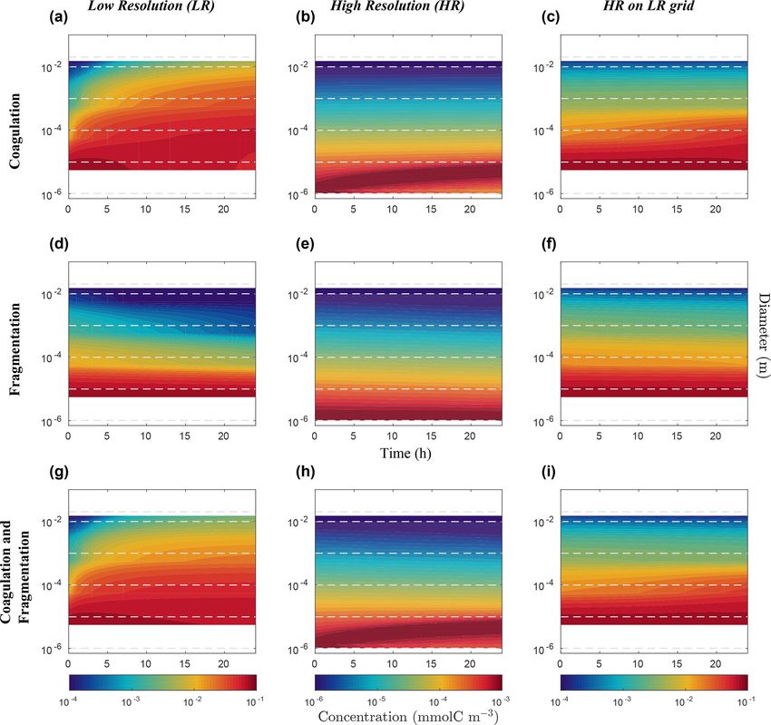
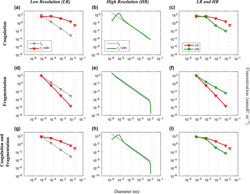
Figure 6. Evolution of the carbon concentration distribution over the size range in our nonlinear size discretization configuration (E2) as
function of diameters. Our three sets of reaction simulations are represented: coagulation only (a–c), fragmentation only (d–f) and when
both reactions are combined (g–i). The left column (a, d, g) represents our LR setup, the middle column (b, e, h) the HR one and the right
column (c, f, i) the comparison of the HR carried back to LR (see Eq. 25 in Sect. 3.1 for details). Y abscissas are different between our
resolutions and are set to allow an easy comparison. For each panel, the initial time step t0 is in black and the final time step t1 = 24 h appears
in red for LR and in green for HR. Solitary points represent the size bin 23 N for both resolutions, as they represent the average of a larger
number of size bins (LR: 5 to 8, and HR: 401 to 800) than the ones in the resolved range. Notice that the final carbon concentration in
the unresolved bin of the HR experiment is divided by a factor of 100 in order to fit in the y scale. As detailed in the methods (Sect. 2.3),
both coagulation and fragmentation reactions occur in the resolved range but only fragmentation occurs in the unresolved range. For further
details, refer to the legend of Fig. 4.
These results demonstrate that in a linearly size discretized of magnitude (Eq. 26, Table 2). In this case, results differ
configuration, the model is reasonably independent of the as a function of resolution for the reactions taken separately
resolution when coagulation and fragmentation are used in- or combined. All LR simulations (K, F and KF) react more
dependently or combined (Fig. 5). They show however the strongly than the HR ones.
importance of considering the unresolved size range in the Focusing first on the resolved range in the coagulation-
model design, which guarantees mass conservation and un- only experiment, we observe a diminution of Cp in the
bounded growth due to coagulation. smaller size bins and an accumulation in the larger size bins
in LR simulation (Fig. 6a). However in HR, this distribution
4.2 Nonlinear discretization pattern is limited to a small range of sizes between 10−6 m
and 10−4 m (Fig. 6b). In addition, no significant accumula-
We now consider the results from the nonlinear size dis- tion of concentration is observed in the largest size bins, and
cretization model (E2), shown in Figs. 6 and 7. Recall that by extension neither into the unresolved range (p = 32 N).
instead of a uniform Cp distribution, the model is initialized This leads to a difference of Cp regarding the larger size
with a distribution that is exponentially decreasing over a bins between LR and HR when mapped on the same grid
size range from 10−6 m to 10−2 m, thus spanning 4 orders (Fig. 6c), with the LR overestimating carbon concentration
Geosci. Model Dev., 14, 4535–4554, 2021 https://doi.org/10.5194/gmd-14-4535-2021G. Gremion et al.: A discrete interaction numerical model for coagulation and fragmentation 4547 Figure 7. Hovmöller plots of carbon concentration as a function of particle diameter over a 24 h period for the nonlinearly discretized configuration (E2). Simulations for coagulation and fragmentation considered separately (on top and middle lines, respectively) and combined (on bottom line), and for LR (left column) and HR (middle column), are shown. The right column shows the HR when mapped to the LR grid. Note the logarithmic scale for the vertical axis representing particle diameter (m) and for the colour scale representing carbon concentrations (mmol C m−3 ). Concentration value scales are different between our resolutions and are set to allow an easy comparison. Dashed lines represent the bounds of each LR size bin. Dealing with size spectrum logarithmic scale, middle size bin concentration value will induce no concentration data in the lower bound of the first size bin in the LR (a, d, g) and for the HR mapped to the LR grid (c, f, i). for larger size bins. Figure 7 shows the time evolution of the tation to explain most of the observed changes in distribu- distributions of Fig. 6. In the LR case, the initial response tion of the LR simulation (Fig. 6g). In HR, both coagulation (roughly 2 h) is characterized by a fast timescale, followed by and fragmentation have localized effects on the smallest and a slower response during the rest of the simulation (Fig. 7a). largest size ranges (Fig. 6h). The comparison of HR vs. LR In contrast, in the HR case, the response is localized in the shows a pattern that is similar to the comparison between small size range and only the slower response is observed resolutions for the coagulation reaction (Figs. 6i and 7i). (Fig. 7b). While attenuated, these biases are still clearly visi- This indicates that coagulation dominates over fragmenta- ble when HR is remapped on LR (Fig. 7c). tion, which is expected for an initial concentration distribu- Results for fragmentation only yield a similar biases be- tion that is highly skewed towards small particles. tween the LR and HR cases. Reactions are magnified in LR These simulations demonstrate that when using a nonlin- compared to HR (panels d–f of Figs. 6 and 7). When both re- ear size discretization and a nonlinear initial carbon concen- actions are combined, coagulation dominates over fragmen- tration distribution, the model behaviour is significantly de- https://doi.org/10.5194/gmd-14-4535-2021 Geosci. Model Dev., 14, 4535–4554, 2021
4548                           G. Gremion et al.: A discrete interaction numerical model for coagulation and fragmentation

Figure 8. Evolution of the carbon concentration distribution over the size range in our nonlinear size discretization configuration (E2) as
function of diameters when the function reducing resolution dependency is implemented (Eq. 27). Our three sets of reaction simulations
are represented: coagulation only (a–c), fragmentation only (d–f) and when both reactions are combined (g–i). The left column (a, d, g)
represents our LR setup, the middle column (b, e, h) the HR one and the right column (c, f, i) the comparison of the HR carried back to LR
(see Eq. 25 in Sect. 3.1 for details). For each panel, the initial time step t0 is in black and the final time step t1 = 24 h appears in red for LR
and in green for HR. For further details, refer to the legend of Fig. 6.

pendent on resolution. To attenuate this dependence, which                  with λ5 and λ6 positive constant parameters that were deter-
arises from the asymmetry between coagulation and frag-                     mined empirically (see Table 1).
mentation, we propose adding and tuning a penalty function                     Simulation results obtained with this correction factor
that will compensate this difference as N varies.                           (Figs. 8 and 9) show that both LR and HR simulations now
                                                                            agree much better. The LR simulation is the one that is the
4.3    Resolution dependency function                                       most impacted by this change (Fig. 8a–c), as f (N = 400) =
                                                                            0.9878 and f (N = 4) = 0.0526. Comparing Fig. 6c, f and i
The residual dependence of the model to resolution in the                   with Fig. 8c, f and i, it is clear that a carefully chosen penalty
nonlinear discretization arises mainly from the fact that the               function such as that in Eq. (27) can significantly reduce the
prefactors used in Eq. (22) are derived from a linear anal-                 error attributed to a number of size bins as low as four. The
ysis, which yields an asymmetry between coagulation and                     fundamental cause of the resolution dependency seems to be
fragmentation. To minimize the effect of this asymmetry,                    linked with the nonlinear size discretization, but it is not clear
we propose multiplying both reaction terms by a resolution-                 how the penalty function can be determined in a simple way
dependent function f (N ) that is positive and monotonically                from prior knowledge. Is this solely dependent on the choice
varies between a value to be determined at low N and 1                      of discretization, or is it also dependent on how particles are
for N → ∞. For simplicity, we here assume an exponential                    distributed along that spectrum? This remains an open ques-
function of the form                                                        tion.

f (N ) = 1 − λ5 e−λ6 N ,                                         (27)

Geosci. Model Dev., 14, 4535–4554, 2021                                                        https://doi.org/10.5194/gmd-14-4535-2021
G. Gremion et al.: A discrete interaction numerical model for coagulation and fragmentation 4549
Figure 9. Hovmöller plots of carbon concentration as a function of particle diameter over a 24 h period for the nonlinearly discretized
configuration (E2) with the application of the function which attempt to reduce the dependency to the resolution of our model (Eq. 27).
Simulations for coagulation and fragmentation considered separately (on top and middle lines, respectively) and combined (on bottom line),
and for LR (left column) and HR (middle column), are shown. For further details, refer to the legend of Fig. 7.
5 Summary fers (i) boundaries to avoid any exponential growth of the
size range and (ii) reduces falsified carbon concentration es-
We have developed a new 0-D numerical model for repre- timation in the larger size bins. When absent, accumulation
senting coagulation and fragmentation as an interaction be- of particles was observed (exploratory studies of our current
tween three particles of arbitrary sizes. Particles are cate- work which are not shown). This caveat is present in mod-
gorized in size bins that can be linearly or nonlinearly dis- els using the sectional approach, the solution of which is to
tributed along a given size spectrum. In the linear configu- increase the number of bins, as described by Burd (2013).
ration, E1, the total volume of suspended particulate matter Coagulation has a quadratic dependence on particle num-
(i.e. the sum of the volume of all individual particles) is also ber concentration participating to the reaction, while frag-
conserved. However, this is not strictly the case in the nonlin- mentation has a linear dependence on the particle number
ear configuration, E2, because it can happen that two parti- concentration. The linear configuration has a very weak de-
cles of two different size bins can end up in the same size bin pendence on the size spectral resolution (number of size bins
as the biggest one. By construction, the total concentration N for a given size range). The nonlinear configuration has a
of carbon carried by particles is conserved over the resolved significant dependence to resolution. This dependence can be
and unresolved range. The unique arbitrary size bin 32 N of-
https://doi.org/10.5194/gmd-14-4535-2021 Geosci. Model Dev., 14, 4535–4554, 2021You can also read