Data-driven models of dominantly-inherited Alzheimer's disease progression - bioRxiv
←
→
Page content transcription
If your browser does not render page correctly, please read the page content below
bioRxiv preprint first posted online Jan. 19, 2018; doi: http://dx.doi.org/10.1101/250654. The copyright holder for this preprint
 (which was not peer-reviewed) is the author/funder, who has granted bioRxiv a license to display the preprint in perpetuity.
                              It is made available under a CC-BY-NC-ND 4.0 International license.

         Data-driven models of dominantly-inherited Alzheimer’s disease
                                  progression
            Neil P. Oxtobya,∗, Alexandra L. Younga , David M. Cashb , Tammie L. S. Benzingerc ,
         Anne M. Faganc , John C. Morrisc , Randall J. Batemanc , Nick C. Foxb , Jonathan M. Schottb ,
                                            Daniel C. Alexandera
     a
      Progression Of Neurological Disease group, Centre for Medical Image Computing and Department of Computer
                        Science, University College London, London WC1E 6BT, United Kingdom
    b
      Dementia Research Centre, Department of Neurodegenerative Disease, Institute of Neurology, University College
                                     London, London WC1E 6BT, United Kingdom
      c
        The Dominantly Inherited Alzheimer Network, Washington University School of Medicine, St Louis, MO, USA

  Abstract
  Dominantly-inherited Alzheimer’s disease is widely hoped to hold the key to developing inter-
  ventions for sporadic late onset Alzheimer’s disease. We use emerging techniques in generative
  data-driven disease-progression modelling to characterise dominantly-inherited Alzheimer’s dis-
  ease progression with unprecedented resolution, and without relying upon familial estimates of
  years until symptom onset (EYO). We retrospectively analysed biomarker data from the sixth data
  freeze of the Dominantly Inherited Alzheimer Network observational study, including measures of
  amyloid proteins and neurofibrillary tangles in the brain, regional brain volumes and cortical thick-
  nesses, brain glucose hypometabolism, and cognitive performance from the Mini-Mental State
  Examination (all adjusted for age, years of education, sex, and head size, as appropriate). Data
  included 338 participants with known mutation status (211 mutation carriers: 163 PSEN1; 17
  PSEN2; and 31 APP) and a baseline visit (age 19–66; up to four visits each, 1·1 ± 1·9 years in
  duration; spanning 30 years before, to 21 years after, parental age of symptom onset). We used an
  event-based model to estimate sequences of biomarker changes from baseline data across disease
  subtypes (mutation groups), and a differential-equation model to estimate biomarker trajectories
  from longitudinal data (up to 66 mutation carriers, all subtypes combined). The two models concur
  that biomarker abnormality proceeds as follows: amyloid deposition in cortical then sub-cortical
  regions (approximately 24±11 years before onset); CSF p-tau (17±8 years), tau and Aβ42 changes;
  neurodegeneration first in the putamen and nucleus accumbens (up to 6 ± 2 years); then cognitive
  decline (7 ± 6 years), cerebral hypometabolism (4 ± 4 years), and further regional neurodegenera-
  tion. Our models predicted symptom onset more accurately than EYO: root-mean-squared error of
  1·35 years versus 5·54 years. The models reveal hidden detail on dominantly-inherited Alzheimer’s
  disease progression, as well as providing data-driven systems for fine-grained patient staging and
  prediction of symptom onset with great potential utility in clinical trials.
  Keywords: event-based model, differential-equation model, disease progression,
  dominantly-inherited Alzheimer’s disease, biomarker dynamics

         ∗
             Corresponding author: Neil Oxtoby, University College London, UK: neiloxtoby.com

  Preprint submitted to Brain (Author’s Original Version)                                                                      2017-05-22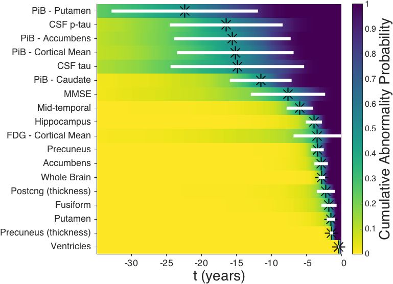
bioRxiv preprint first posted online Jan. 19, 2018; doi: http://dx.doi.org/10.1101/250654. The copyright holder for this preprint
 (which was not peer-reviewed) is the author/funder, who has granted bioRxiv a license to display the preprint in perpetuity.
                              It is made available under a CC-BY-NC-ND 4.0 International license.

  1. Introduction
       Understanding and identifying the earliest pathological changes of Alzheimer’s disease is key
  to realizing disease-modifying treatments, which are likely to be most efficacious when given
  early. However, identifying individuals in the presymptomatic stage of typical, sporadic, late on-
  set Alzheimer’s disease is challenging. Therefore, there is considerable interest in investigating
  dominantly-inherited Alzheimer’s disease, which is caused by mutations in the Amyloid Precur-
  sor Protein (APP), Presenilin 1 (PSEN1), and Presenilin 2 (PSEN2) genes, and which provides the
  opportunity to identify asymptomatic “at risk” individuals prior to the onset of cognitive decline
  for observational studies and clinical trials. Although considerably rarer than sporadic Alzheimer’s
  disease, dominantly-inherited Alzheimer’s disease has broadly similar clinical presentation (Tang
  et al., 2016, Ryan et al., 2016), i.e., episodic memory followed by further cognitive deficits, and
  both display heterogeneity in terms of symptoms and progression, much of which is unexplained
  (Bateman et al., 2010). An important question when attempting to extrapolate biomarker dynam-
  ics (and in due course clinical trials results) between dominantly-inherited Alzheimer’s disease
  and sporadic Alzheimer’s disease, is whether presymptomatic changes in dominantly-inherited
  Alzheimer’s disease mirror those in sporadic Alzheimer’s disease, as might be expected given the
  broad similarities in pathological features across both diseases (Bateman et al., 2010, Weiner et al.,
  2012, Morris et al., 2012, Cairns et al., 2015).
       Most previous investigations into dominantly-inherited Alzheimer’s disease progression used
  traditional regression models to explore the time course of Alzheimer’s disease markers as a func-
  tion of estimated years to onset (EYO) of clinical symptoms, based on age of onset (Ryman et al.,
  2014) in affected first-degree relatives. In 2012, this type of cross-sectional analysis of biomarker
  trajectories in the Dominantly Inherited Alzheimer Network (DIAN) observational study estimated
  the following sequence of pre-symptomatic biomarker changes (Bateman et al., 2012): measures of
  beta-amyloid (Aβ) in cerebrospinal fluid (CSF) and in amyloid imaging using Pittsburgh-compound
  B PET (PiB-PET); CSF levels of tau; regional brain atrophy; cortical glucose hypometabolism in
  flurodeoxyglucose PET (FDG-PET); episodic memory; Mini Mental State Examination (MMSE)
  score (Folstein et al., 1975); and Clinical Dementia Rating Sum of Boxes (CDRSUM) score (Berg,
  1988). Results of a more recent model-based analysis (Fleisher et al., 2015) showed a similar
  progression sequence in the Alzheimer’s Prevention Initiative Colombian cohort, all of whom
  carry the same mutation (E280A PSEN1). In 2013, a more detailed investigation of imaging
  biomarkers (Benzinger et al., 2013) observed regional variability in the cross-sectional sequence
  of biomarker changes: some grey-matter structures having amyloid plaques may not later lose
  metabolic function, and others may not atrophy. Various other studies of dominantly-inherited
  Alzheimer’s disease have reported early behavioural changes (Ringman et al., 2015) and pre-
  symptomatic within-individual atrophy (Cash et al., 2013) in brain regions commonly associated
  with sporadic Alzheimer’s disease, and additionally in the putamen and thalamus. The key feature
  in each of these studies of dominantly-inherited Alzheimer’s disease progression is the reliance
  upon EYO, which is typically based upon the estimated age at which an individual’s affected parent
  first shows progressive cognitive decline (Bateman et al., 2010), or upon the average age of onset
  for a mutation type (Ryman et al., 2014). The parental estimate of familial age of onset is generated
  by a semi-structured interview and is known to be inherently uncertain both because of uncertain-
  ties in estimating when an individual is deemed to be affected, and because there can be substantial
  within-family and within-mutation differences in actual age of onset (Ryman et al., 2014). This

                                                                      2
bioRxiv preprint first posted online Jan. 19, 2018; doi: http://dx.doi.org/10.1101/250654. The copyright holder for this preprint
(which was not peer-reviewed) is the author/funder, who has granted bioRxiv a license to display the preprint in perpetuity.
It is made available under a CC-BY-NC-ND 4.0 International license.
uncertainty in EYO limits its utility for estimating disease progression in pre-symptomatic indi-
viduals who carry a dominantly-inherited Alzheimer’s disease mutation: reducing confidence in
predicting onset; and when staging patients — at best reducing the resolution in which biomarker
ordering can be inferred, at worst biasing the ordering. The mutation age of onset addresses higher
variance estimates, and demonstrates good predictability, but is still a retrospective estimate and
not obtained by prospectively monitoring for actual onset of symptoms in a uniform longitudinal
fashion.
Here we take a different approach: generative, data-driven, disease progression modelling.
Data-driven progression models have emerged in recent years as a family of computational ap-
proaches for analyzing progressive diseases. Instead of regressing against pre-defined disease
stages (Bateman et al., 2012, Ridha et al., 2006, Scahill et al., 2002, Yang et al., 2011), or learning
to classify cases from a labelled training database (Klöppel et al., 2008, Mattila et al., 2011, Young
et al., 2013), generative data-driven progression models construct an explicit quantitative disease
signature without the need for a priori staging. Mostly applied to neurodegenerative conditions like
Alzheimer’s disease, results include discrete models of biomarker changes (Fonteijn et al., 2012,
Young et al., 2014, Venkatraghavan et al., 2017), continuous models of biomarker dynamics (Jedy-
nak et al., 2012, Villemagne et al., 2013, Donohue et al., 2014, Oxtoby et al., 2014), spatiotemporal
models of brain image dynamics (Durrleman et al., 2013, Lorenzi et al., 2015, Schiratti et al., 2015,
Huizinga et al., 2016), and models of disease propagation mechanisms (Seeley et al., 2009, Zhou
et al., 2012, Raj et al., 2012, Iturria-Medina et al., 2014, 2017).
In this paper we use two generative data-driven disease progression models to extract patterns of
observable biomarker changes in dominantly-inherited Alzheimer’s disease. We estimate ordered
sequences of biomarker abnormality in disease subtypes (mutation groups) from cross-sectional
data using an event-based model (Fonteijn et al., 2012, Young et al., 2014), and we estimate
biomarker trajectories from short-interval longitudinal data using a nonparametric differential equa-
tion model similar to previous parametric work (Oxtoby et al., 2014, Villemagne et al., 2013). Our
data-driven generative models have several potential advantages over previous models. First, they
are generalizable to non-familial forms of progressive diseases because they do not rely on EYO.
Second, they generate a uniquely detailed sequence of biomarker changes and trajectories. Third,
they support a fine-grained staging and prognosis system of potential direct application to clinical
trials and in clinical practice. We demonstrate the prognostic utility by predicting actual symptom
onset in unseen data more accurately than using EYO.
2. Materials and Methods
We used data-driven models to analyse biomarker data (MRI, PET, CSF, cognitive test scores)
from the DIAN study. From cross-sectional (baseline) data we estimated disease progression se-
quences using an event-based model (Fonteijn et al., 2012, Young et al., 2014). For explicit quan-
tification of disease progression time, we estimated biomarker trajectories from short-term longitu-
dinal data by using covariate-adjusted, nonparametric differential equation models, which offer two
key advantages over previous approaches in (Villemagne et al., 2013, Oxtoby et al., 2014): replac-
ing parametric model-selection with a data-driven approach, and explicitly estimating population
variance in a Bayesian manner. Models were cross-validated internally (see Statistical Analysis
section and Supplementary Material).
3bioRxiv preprint first posted online Jan. 19, 2018; doi: http://dx.doi.org/10.1101/250654. The copyright holder for this preprint
(which was not peer-reviewed) is the author/funder, who has granted bioRxiv a license to display the preprint in perpetuity.
It is made available under a CC-BY-NC-ND 4.0 International license.
2.1. Participants
At the sixth data freeze, the DIAN cohort included 338 individual participants (192 females,
57%) with known mutation status and a baseline visit, aged 19–66 years at baseline (39 ± 10 years),
with up to four visits each (1·1 ± 1·9 years in duration, total of 535 visits), spanning 30 years before
and 21 years after parental age of symptom onset. For detailed descriptive summaries of the DIAN
cohort, we refer the reader to Morris et al. (2012).
2.1.1. Data selection and preparation
Table 1 summarises the demographics of DIAN participants analysed in this work.
We selected 24 Alzheimer’s disease biomarkers based on specificity to the disease, or if dis-
ease ‘signal’ is present, i.e., quantifiable distinction between mutation carriers and non-carriers
(see Statistical Analysis section). The biomarkers include CSF measures of molecular pathol-
ogy (amyloid proteins and neurofibrillary tangles); a cognitive test score (MMSE); regional brain
volumetry from MRI, e.g., hippocampus, middle-temporal region, temporo-parietal cortex; PiB-
PET imaging measures of amyloid accumulation; and FDG-PET imaging measures of glucose
hypometabolism. We excluded imaging data (21 structural scans from 10 participants) having arte-
facts or non-Alzheimer’s disease pathology such as a brain tumour. Of the included participants,
211 (117 females, 55%) were dominantly-inherited Alzheimer’s disease mutation carriers (MC):
163 PSEN1; 17 PSEN2; and 31 APP; and 120 were non-carriers (NC). Baseline data for mutation
carriers and non-carriers was used to fit event-based models. The full set of biomarkers included in
the event-based model is listed on the vertical axis of Figure 1.
Of the 211 included mutation carriers, 66 had longitudinal data suitable for fitting differential
equation models. To reduce the influence of undue measurement noise we excluded biomarker data
with a large coefficient of variation within individuals, e.g., as done for CSF biomarkers in Bateman
et al. (2012). Following Villemagne et al. (2013), we also excluded differential data that was both
normal (beyond a threshold determined by clustering), and non-progressing (rate of change has a
contradictory sign to disease progression, e.g., reverse atrophy or improved cognition). Finally,
we identified six cognitively normal mutation carriers who developed symptoms during the study
(global CDR becoming nonzero after baseline). Since we use our differential equation models
to predict symptom onset for these participants, we excluded them from the model fits to avoid
circularity (including them doesn’t alter our results considerably). This left data from up to 51
mutation carriers (41 PSEN1; 1 PSEN2; 9 APP; 28 females) available for analysis using differential
equation models. Subsets had data for structural imaging (47; 26 females), CSF (32; 16 females),
PiB PET (32; 16 females), and FDG PET (39; 22 females) biomarkers.
We used stepwise regression to remove the influence of age, years of education, sex, and head
size (total intracranial volume, MRI volumes only) prior to fitting our models.
2.2. Models
2.2.1. Cross-sectional: Event-Based Models
The event-based model infers a sequence in which biomarkers show abnormality, together with
uncertainty in that sequence, from cross-sectional data (Fonteijn et al., 2012). This longitudi-
nal picture of disease progression is estimable using this approach because, across the spectrum
of Dominantly Inherited Alzheimer Network study participants from cognitively normal controls
(non-carriers of dominantly-inherited Alzheimer’s disease mutations), to presymptomatic mutation
carriers, and symptomatic patients, more individuals will show higher likelihood of abnormality in
4bioRxiv preprint first posted online Jan. 19, 2018; doi: http://dx.doi.org/10.1101/250654. The copyright holder for this preprint
(which was not peer-reviewed) is the author/funder, who has granted bioRxiv a license to display the preprint in perpetuity.
It is made available under a CC-BY-NC-ND 4.0 International license.
Demographic Non-carriers Mutation carriers [PSEN1, PSEN2, APP]
n analysed, cross-sectional
A. 127 211 [163, 17, 31 (77%, 8%, 15%)]
(event-based models)
Female 75 (59%) 117 [92, 5, 20 (79%, 4%, 17%)]
APOE4-positive 37 (29%) 61 [47, 7, 7 (77%, 11·5%, 11·5%)]
APOE4-negative 90 (71%) 150 [116, 10, 24 (77%, 7%, 16%)]
Age at baseline
39 ± 10 39 ± 10 [39 ± 10, 39 ± 10, 43 ± 10]
± standard deviation, years
Education at baseline
15 ± 3 14 ± 3 [14 ± 3, 15 ± 3, 14 ± 3]
± standard deviation, years
EYO at baseline
−7 ± 12 −7 ± 10 [−7 ± 10, −12 ± 10, −6 ± 9]
± standard deviation, years
Cog: 51 [41, 1, 9 (80%, 2%, 18%)]
MRI: 47 [37, 2, 8 (79%, 4%, 17%)]
n analysed, longitudinal
B. n/a CSF: 32 [28, 1, 3 (88%, 3%, 9%)]
(differential equation models)
PiB: 32 [25, 2, 5 (78%, 6%, 16%)]
FDG: 39 [31, 2, 6 (80%, 5%, 15%)]
Cog: 28 (55%) [21, 1, 6 (75%, 4%, 21%)]
MRI: 26 (55%) [19, 1, 6 (73%, 4%, 23%)]
Female n/a CSF: 16 (50%) [13, 0, 3 (81%, 0%, 19%)]
PiB: 16 (50%) [11, 1, 4 (69%, 6%, 25%)]
FDG: 22 (56%) [16, 1, 5 (73%, 5%, 23%)]
Cog: 17 (33%) [13, 0, 4 (76%, 0%, 24%)]
MRI: 16 (34%) [11, 1, 4 (69%, 6%, 25%)]
APOE4-positive n/a CSF: 8 (25%) [6, 1, 1 (75%, 12·5%, 12·5%)]
PiB: 13 (41%) [9, 1, 3 (69%, 8%, 23%)]
FDG: 14 (36%) [10, 1, 3 (71%, 7%, 21%)]
Cog: 34 (67%) [28, 1, 5 (82%, 3%, 15%)]
MRI: 31 (66%) [26, 1, 4 (84%, 3%, 13%)]
APOE4-negative n/a CSF: 24 (75%) [22, 0, 2 (92%, 0%, 8%)]
PiB: 19 (59%) [16, 1, 2 (84%, 5%, 11%)]
FDG: 25 (64%) [21, 1, 3 (84%, 4%, 12%)]
Cog: 41 ± 10 [40 ± 10, 32 ± 0, 48 ± 7]
MRI: 42 ± 10 [40 ± 10, 45 ± 18, 50 ± 6]
Age at baseline
n/a CSF: 43 ± 9 [42 ± 9, 57 ± 0, 48 ± 8]
± standard deviation, years
PiB: 43 ± 10 [41 ± 10, 45 ± 18, 49 ± 4]
FDG: 42 ± 10 [41 ± 10, 45 ± 18, 48 ± 5]
Cog: 14 ± 2 [14 ± 2, 18 ± 0, 15 ± 2]
MRI: 14 ± 2 [14 ± 2, 15 ± 4, 15 ± 2]
Education at baseline
n/a CSF: 14 ± 3 [14 ± 3, 12 ± 0, 14 ± 3]
± standard deviation, years
PiB: 14 ± 3 [14 ± 2, 15 ± 4, 15 ± 3]
FDG: 14 ± 2 [14 ± 2, 15 ± 4, 15 ± 2]
Cog: −3 ± 7 [−3 ± 7, −19 ± 0, −2 ± 8]
MRI: −2 ± 8 [−3 ± 7, −6 ± 18, 0 ± 6]
EYO at baseline
n/a CSF: 0 ± 7 [0 ± 7, 7 ± 0, −3 ± 6]
± standard deviation, years
PiB: −2 ± 7 [−3 ± 6, −6 ± 18, 0 ± 3]
FDG: −3 ± 7 [−4 ± 7, −6 ± 18, −2 ± 5]
Table 1: Demographics for DIAN participants at Data Freeze 6. A. Cross-sectional data used to build event-based
models of dominantly-inherited Alzheimer’s disease progression. B. Longitudinal data used to build differential equa-
tion models of dominantly-inherited Alzheimer’s disease progression. See Data Selection and Preparation section for
more. Abbreviations: Cog – Cognitive test scores; PiB – Pittsburgh compound B PET data; FDG – fludeoxyglucose
hypometabolism PET data; EYO – estimated years to onset based on parental age of symptom onset.
biomarkers that change early in the progression. Thus, with sufficient representation across com-
binations of abnormal and normal observations, the likelihood of any full ordered sequence can be
estimated to reveal the most likely sequences. The probabilistic sequence of events estimated by
the event-based model is useful for fine-grained staging of individuals by calculating the likelihood
of their data (biomarker observations) arising from each stage of the sequence (Young et al., 2014).
We fit an event-based model to determine the most probable sequence of biomarker abnormality
events and the uncertainty in this sequence for all but 3 of the 24 biomarkers described previously:
5bioRxiv preprint first posted online Jan. 19, 2018; doi: http://dx.doi.org/10.1101/250654. The copyright holder for this preprint
(which was not peer-reviewed) is the author/funder, who has granted bioRxiv a license to display the preprint in perpetuity.
It is made available under a CC-BY-NC-ND 4.0 International license.
measurements of entorhinal cortex, thalamus, and caudate volume were excluded on the basis that
they did not show significant differences (see Statistical Analysis section) between non-carriers and
symptomatic mutation carriers after correction for age, sex, education and total intracranial volume.
Each event represents the transition of a biomarker from a normal level (as seen in non-carriers)
to an abnormal level (as seen in symptomatic patients). The probability a biomarker measurement
is normal is modelled as a Gaussian distribution, and estimated using data from non-carriers. The
distribution of abnormal measurements is also modelled as a Gaussian distribution, but estimated by
fitting a mixture of two Gaussians (Fonteijn et al., 2012) to data from all mutation carriers: the first
Gaussian models the distribution of normal measurements, and is kept fixed to the values estimated
from non-carriers; the second Gaussian models the distribution of abnormal measurements, and
is optimised using data from mutation carriers. The sequence of events was estimated in various
population subgroups: all 211 mutation carriers; 163 PSEN1 mutation carriers; 17 PSEN2 mutation
carriers; and 31 APP mutation carriers. We also considered separate event-based models by APOE4
status: 61 mutation carriers who were APOE4-positive (with one or more APOE4 alleles), and 150
mutation carriers who were APOE4-negative. For further details of the model fitting procedures,
see the Statistical Analysis section. We assigned participants to patient stages based on their most
probable position along the most probable event sequence (Young et al., 2014) for all mutation
carriers combined. We assessed the efficacy of the patient staging system using only participants
with data available for all biomarkers (n = 30, total of 42 follow-up visits), as missing entries cause
uncertainty in a participant’s model stage.
2.2.2. Longitudinal: Differential Equation Models
Reconstruction of biomarker trajectories ideally requires dense longitudinal data collected over
the full time course of the disease. Such data is not yet available due to the prohibitive expense and
complexity of collection, which means that we must resort to alternative methods. In dominantly-
inherited Alzheimer’s disease and other neurodegenerative diseases, the availability of short-term
longitudinal data of a few years permits estimation of an individual’s rate of change over that time
span, e.g., via linear regression. These short-interval longitudinal observations are interpreted as
noisy samples (segments) from an average biomarker trajectory. Instead of attempting to align
the raw data segments, e.g., (Donohue et al., 2014), they are used to generate a cross-section of
differential data: biomarker rate-of-change as a function of biomarker value, i.e., a differential
equation. For sufficient coverage across a range of biomarker values tracking dominantly-inherited
Alzheimer’s disease progression, the function can be integrated to produce a trajectory. The tech-
nique estimates probabilistic trajectories that are useful for predicting symptom onset (with confi-
dence bounds) for an individual by aligning their biomarker observations to the trajectory. We refer
to this approach as a differential equation model, since it is analogous to the numerical integration
of ordinary differential equations as performed in many fields of science.
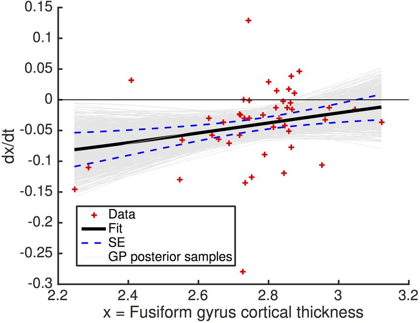
Here we took a univariate approach, considering each biomarker in turn. We found each indi-
vidual’s biomarker rate-of-change, dx/dt, through linear regression of their short-term longitudinal
data. We then plotted this against average biomarker value x (for each individual), and fit a curve
f (x)
dx
= f (x) + ε (1)
dt
with residual errors ε. Finally, we numerically integrated along the fitted DEM curve C between
6bioRxiv preprint first posted online Jan. 19, 2018; doi: http://dx.doi.org/10.1101/250654. The copyright holder for this preprint
(which was not peer-reviewed) is the author/funder, who has granted bioRxiv a license to display the preprint in perpetuity.
It is made available under a CC-BY-NC-ND 4.0 International license.
biomarker extreme values a and b to estimate a model of the average trajectory
Z b
x(t) = a + dx (2)
a
I
1
t= dx (3)
C f (x)
Previously, Villemagne et al. (2013) took a model-selection approach to finding the best fitting
polynomial regression model for f (x). Instead, we use a nonparametric Bayesian approach (see
Statistical Analysis section).
In dominantly-inherited Alzheimer’s disease, biomarker trajectories are usually investigated as
a function of EYO. This is an approximate proxy for disease progression time where EYO = 0 is
the estimated point of onset of clinical symptoms, based on familial age of onset such as that of
an affected parent. Here we defined t = 0 at a data-driven canonical abnormal level: the median
biomarker value for symptomatic participants in the DIAN cohort (first symptomatic visit).
A quantity of clinical interest is the interval of time between normal and abnormal biomarker
levels, which we refer to as the Abnormality Transition Time, and define in a data-driven manner
via median values for asymptomatic (canonically normal) and symptomatic (canonically abnormal
as above) participants in the DIAN dataset. Our probabilistic approach produces an abnormality
transition time distribution per biomarker. The cumulative probability of abnormality produces
data-driven sigmoid-like curves, which we combine across biomarkers to estimate a temporal pat-
tern of disease progression.
We estimated time to onset (ETO) for each individual as a weighted average across biomarkers.
Aligning each biomarker measurement to each biomarker trajectory produces a set of biomarker-
specific ETOs with credible intervals. We weighted by the inverse width of the credible interval,
to assign lower confidence to estimates with large uncertainty. Incomplete data was used, with
missing values omitted from the weighted average.
2.3. Statistical Analysis
For fitting the event-based model we followed the same procedures as in Young et al. (2014).
Briefly, the characteristic sequence and its uncertainty is estimated through a Markov chain Monte
Carlo sampling procedure with greedy-ascent initialisation for maximising the data likelihood
(Fonteijn et al., 2012). We used a noninformative uniform prior on the sequence. When fitting
an event-based model, it is important to select a set of biomarkers specific to the disease. That
is, where disease ‘signal’ is present: a quantifiable distinction between normal and abnormal. For
this procedure we used a paired t-test, and thresholded significance at p < 0.01/24, Bonferroni-
corrected for multiple comparisons. We accounted for missing data by imputing biomarker values
such that missing measurements had an equal probability of being normal or abnormal (Young
et al., 2015), and thus would not influence the population sequence. We performed cross-validation
of the event-based model by re-estimating the event distributions and maximum likelihood se-
quence for 100 bootstrap samples from each data subset. The positional variance diagrams for the
cross validation results show the proportion of bootstrap samples in which event i (vertical axis)
appears at position k (horizontal axis) of the maximum likelihood sequence.
For fitting differential equation models we use a nonparametric approach known as Gaussian
process regression (Rasmussen and Williams, 2006) to produce a probabilistic fit (a distribution
7bioRxiv preprint first posted online Jan. 19, 2018; doi: http://dx.doi.org/10.1101/250654. The copyright holder for this preprint
(which was not peer-reviewed) is the author/funder, who has granted bioRxiv a license to display the preprint in perpetuity.
It is made available under a CC-BY-NC-ND 4.0 International license.
of curves) that is determined by the data. The fitting was implemented within the probabilistic
programming language Stan (Stan Development Team, 2015), which performs full Bayesian sta-
tistical inference using Markov chain Monte Carlo sampling and penalized maximum likelihood
estimation. We used a vanilla squared-exponential kernel (Rasmussen and Williams, 2006) for
2
the Gaussian process prior covariance: ki, j (x) = η2 exp −ρ2 xi − x j + δi j σ2 with hyperparam-
eters η, ρ, σ and Kronecker delta function δ. The Gaussian process prior hyperparameters guide
the shape of the regression function, f (x), and were also estimated from the data. Here we used
weakly-informative broad half-Cauchy hyperparameter priors, and diffuse initial conditions to aid
model identifiability. To check for over-fitting we performed 10-fold cross-validation (see Supple-
mentary Material), and various posterior predictive checks to assess model quality and numerical
convergence (Gelman et al., 2014, Vehtari et al., 2016).
3. Results
We first present our cross-sectional multimodal modelling of the fine-grained ordering of dominantly-
inherited Alzheimer’s disease biomarker abnormality using an event-based model. We then present
our longitudinal modelling of dominantly-inherited Alzheimer’s disease biomarker trajectories us-
ing differential equation models.
3.1. Cross-sectional results: event-based models of biomarker abnormality sequences
Figure 1 is a positional variance diagram of the maximum likelihood sequence of biomarker
abnormality events (top to bottom), and its uncertainty (left to right), across all available 211 mu-
tation carriers in the DIAN dataset. Grayscale intensity represents confidence in each event’s po-
sition within the sequence, and is calculated from Markov chain Monte Carlo samples from the
event-based model (Young et al., 2014). The closer this diagram is to a black diagonal, the more
confidence there is in the disease progression sequence.
The event-based model reveals a distinct sequence of biomarker abnormality in dominantly-
inherited Alzheimer’s disease: regional (cortical then striatal) amyloid deposition on PiB-PET
scans; CSF measures of neuronal injury (total tau), neurofibrillary tangles (phosphorylated tau),
and amyloid plaques (Aβ42 and Aβ40/Aβ42 ratio); MRI measures of volume loss in the putamen
and nucleus accumbens; global cognition (MMSE score). Thereafter the ordering in which FDG-
PET hypometabolism and other MRI measures become abnormal is less certain. We found high
certainty early in the ordering of these biomarkers (as reflected by the more solid blocks along the
diagonal), with lower certainty later in the ordering of regional volumes (more diffuse grey blocks
straying from the diagonal). This pattern (left) persists under cross-validation (right).
We also fit the event-based model to subgroups of the mutation carriers in the DIAN data
set. Figure 2 shows positional variance diagrams of the biomarker abnormality event sequence
in APOE4-positive and APOE4-negative participants (those with and without an apolipoprotein-
4 allele), and for the three dominantly-inherited Alzheimer’s disease mutation types in DIAN:
PSEN1, PSEN2, and APP. For ease of comparison, the sequence ordering on the vertical axes of
each plot was chosen to be the most probable ordering from Figure 1 (all mutation carriers). Cross
validation results for Figure 2 are shown in Supplementary Figure 1.
Broadly speaking, we see good agreement of the event sequences across APOE4 subgroups
and across mutation type subgroups in Figure 2, with some subtle differences between groups:
earlier CSF Aβ42 and Aβ40/Aβ42 ratio in the APOE4-positive and APP groups; earlier volume
8bioRxiv preprint first posted online Jan. 19, 2018; doi: http://dx.doi.org/10.1101/250654. The copyright holder for this preprint
(which was not peer-reviewed) is the author/funder, who has granted bioRxiv a license to display the preprint in perpetuity.
It is made available under a CC-BY-NC-ND 4.0 International license.
Figure 1: Event-based model progression of dominantly-inherited Alzheimer’s disease progression. Positional
variance diagrams. Left: event-based model estimated on all mutation carriers in the DIAN dataset. Right: cross-
validation through bootstrapping. The vertical ordering (top to bottom) is given by the maximum likelihood sequence
estimated by the model. Grayscale intensity represents posterior confidence in each event’s position (each row), from
Markov chain Monte Carlo samples of the posterior.
abnormality in the fusiform gyrus for the PSEN2 group; earlier putamen volume abnormality for
the APP group. The uncertainty is high in the subgroup orderings due in part to the low numbers
of participants in these groups, which reduces power to draw concrete conclusions based on these
subtle differences between groups.
Figure 3 demonstrates the fine-grained staging capabilities of the event-based model. Using
the model for all mutation types (Figure 1), each participant in the DIAN dataset was assigned a
disease stage that best reflects their measurements (see Materials and Methods section, and Young
et al. (2014)). The staging proportions are shown in Figure 3(a), differentiated by broad diagnos-
tic groups (CN: Cognitively Normal, global CDR = 0; MCI: very mild dementia consistent with
Mild Cognitive Impairment, global CDR = 0·5; AD: probable dementia due to Alzheimer’s disease,
global CDR > 0·5). Longitudinal consistency of staging is shown in Figure 3(b) where each par-
ticipant’s baseline stage is plotted against available follow-up stages between baseline and months
12/24/36.
The baseline staging in Figure 3(a) shows good separation of diagnostic groups: all of the non-
carriers are assigned to stage 0 (black), CN mutation carriers (green) are at earlier model stages,
mutation carriers diagnosed with probable Alzheimer’s disease dementia (red) are at late model
stages, and mutation carriers with very mild dementia consistent with MCI (blue) are more spread
out across the stages. Within carriers, the model shows high classification accuracy for separating
those who are cognitively normal from those with probable dementia: a balanced accuracy of 93%
is achieved by classifying participants above stage 10 (putamen volume abnormality) as having
probable Alzheimer’s disease dementia. This shows that our generative model can also be used
for discriminative applications with performance comparable to state-of-the-art multimodal binary
classifiers (Willette et al., 2014). Further, Supplementary Figure 15(a) shows positive associations
between baseline EYO and baseline event-based model stage, by diagnostic group.
The follow-up staging in Figure 3(b) shows good longitudinal consistency: at 32 of 36 (89%)
9bioRxiv preprint first posted online Jan. 19, 2018; doi: http://dx.doi.org/10.1101/250654. The copyright holder for this preprint
(which was not peer-reviewed) is the author/funder, who has granted bioRxiv a license to display the preprint in perpetuity.
It is made available under a CC-BY-NC-ND 4.0 International license.
(a) APOE4-positive mutation carriers (n = 61) (b) APOE4-negative mutation carriers (n = 150)
(c) PSEN1 mutation carriers (n = 163) (d) PSEN2 mutation carriers (n = 17) (e) APP mutation carriers (n = 31)
Figure 2: Event-based models of dominantly-inherited Alzheimer’s disease: mutation groups. Data-driven se-
quences of biomarker abnormality shown as positional variance diagrams for mutation carriers in the DIAN dataset
who are (a) APOE4-positive; (b) APOE4-negative; (c) PSEN1 mutation carriers; (d) PSEN2 mutation carriers; (e) APP
mutation carriers. Compare with Figure 1 (all groups combined): similar ordering, with a notable difference: APOE4-
positive participants and APP mutation carriers both showed earlier CSF Aβ42 abnormality. See Supplementary Figure
1 for cross-validation results.
follow-up time points the model stage is the same or it increased; at 34 of 36 (94%) follow-up
time points the stage was either unchanged, it increased, or it decreased within the uncertainty
of the ordering. This included the clinical converters, which are shown with triangles (CN to
MCI in green; MCI to AD in red). The remaining two follow-up time points at which the model
stage decreased (green circles in Figure 3(b); 1 PSEN1, 1 APP) have inconsistent amyloid levels
between CSF and regional PiB-PET, potentially due to discord between these biomarkers as has
been observed in some individuals (Landau et al., 2013, Schroeter et al., 2015).
3.2. Longitudinal results: biomarker trajectories from differential equation models
Figure 4 shows a selection of dominantly-inherited Alzheimer’s disease biomarker trajectories
estimated from the DIAN dataset using our approach. Each average trajectory is shown as a heavy
10bioRxiv preprint first posted online Jan. 19, 2018; doi: http://dx.doi.org/10.1101/250654. The copyright holder for this preprint
(which was not peer-reviewed) is the author/funder, who has granted bioRxiv a license to display the preprint in perpetuity.
It is made available under a CC-BY-NC-ND 4.0 International license.
(a) Staging of participants in the DIAN dataset (b) Staging consistency
Figure 3: Event-based model staging results for dominantly-inherited Alzheimer’s disease. (a) Proportions
grouped by diagnostic group: all noncarriers are at stage zero (black), and advancing disease stage is correlated strongly
with cognitive impairment (green to blue to red). (b) Staging consistency across visits within three years of baseline for
the n = 30 participants having complete longitudinal data (18 mutation carriers; 16 PSEN1, 2 APP). Most participants
advance to a later stage (disease progresses towards the right). Green circles show the two participants (1 PSEN1, 1
APP) who regressed to earlier event-based model stages, which arises in both cases due to discordant amyloid measure-
ments between CSF and PiB-PET. The triangles indicate clinical progressors (CN to MCI in blue; MCI to AD in red).
BL: baseline; M: month; CN: Cognitively Normal (global CDR = 0); MCI: very mild dementia consistent with Mild
Cognitive Impairment (global CDR = 0·5); AD: probable dementia due to dominantly-inherited Alzheimer’s disease
(global CDR > 0·5).
dashed black line, with uncertainty indicated by thin grey trajectories sampled from the posterior
distribution. The time axis is defined such that t = 0 corresponds to the median biomarker value
for symptomatic mutation carriers (sMC) in the DIAN dataset, which we define as the canonical
abnormal level. This is marked in Figure 4 by a red horizontal line for each biomarker, with the
corresponding distribution of biomarker values for sMC shown to the left of each trajectory as a
red quartile box plot. The green quartile box plots show the biomarker distributions for asymp-
tomatic mutation carriers (aMC), with the median value for each biomarker defining our canonical
normal level and shown by a green horizontal line. Importantly, the canonical normal and abnormal
levels are not required to estimate the biomarker trajectories, but are used to define the Abnormal-
ity Transition Time for each biomarker as a data-driven estimate of the duration of the transition
between these levels. Our Bayesian approach estimates an Abnormality Transition Time density
(probability distribution) for each biomarker, which is shown in blue in Figure 4. For comparison,
linear mixed model fits to baseline DIAN data from Bateman et al. (2012) are shown in magenta in
Figure 4(b)/(c)/(d)/(e) (others not available).
Most trajectories in Figure 4 (and in Supplementary Material) show acceleration from normal to
abnormal levels, with little evidence for post-onset deceleration/plateauing that would be consistent
with the sigmoidal behaviour hypothesized for sporadic Alzheimer’s disease in, e.g., Jack et al.
(2010). Biomarkers with trajectories that do not plateau, but remain dynamic into the symptomatic
phase of the disease, offer potential utility for monitoring progression later in the disease. The grey
curves capture uncertainty in the biomarker dynamics which arises both from fitting the differential
equation models to discrete data, and from heterogeneity in the population. For comparison with
our data-driven approach, the magenta trajectories in Figure 4(b)/(c)/(d)/(e) are from Bateman et al.
(2012), which used regression of baseline data against EYO. Qualitatively, they broadly agree with
11bioRxiv preprint first posted online Jan. 19, 2018; doi: http://dx.doi.org/10.1101/250654. The copyright holder for this preprint
(which was not peer-reviewed) is the author/funder, who has granted bioRxiv a license to display the preprint in perpetuity.
It is made available under a CC-BY-NC-ND 4.0 International license.
our trajectories for PiB-PET (cortical average amyloid deposition), MMSE, Hippocampus volume,
and FDG-PET (cortical average hypometabolism), although, around symptom onset and beyond,
our steeper Hippocampus volume trajectory implies a more aggressive progression than estimated
cross-sectionally in Bateman et al. (2012).
(a) CSF p-tau (b) PiB-PET cortical mean SUVR (c) MMSE score
(d) Hippocampus volume (e) FDG-PET cortical mean SUVR (f) Putamen volume
Figure 4: Differential equation models: dominantly-inherited Alzheimer’s disease biomarker trajectories. Shown
are fits for selected biomarkers (see Models section). Fits for other biomarkers are provided in the Supplementary Mate-
rial. Heavy black dashed lines show the average trajectory, with grey lines showing trajectories sampled from the poste-
rior distribution. Time is expressed relative to the median biomarker value (red line) for symptomatic mutation carriers
in the DIAN dataset (first visit with a nonzero CDR score), so that negative time suggests the average pre-symptomatic
phase of dominantly-inherited Alzheimer’s disease. Box plots show biomarker distributions for asymptomatic (green,
left, canonical normal) and symptomatic (red, right, canonical abnormal) mutation carriers (denoted aMC and sMC,
respectively), with the distribution for estimated time between canonical normal and canonical abnormal (Abnormality
Transition Time) shown in blue. Details of included participants are given in Table 1. For comparison, the magenta fits
in (b), (c), (d), and (e) are those from the linear mixed models of baseline DIAN data against EYO from Bateman et al.
(2012). SUVR = standardized uptake value ratio (relative to the cerebellum).
Figure 5 shows the cumulative probability for each biomarker in Figure 4. That is, the empirical
distribution function for the Abnormality Transition Time densities in Figure 4, using the same time
axis but on a logarithmic scale to ease visualisation. From Figure 5 we can infer an ordering of
abnormality (Figure 5 legend) by comparing the times at which each curve reaches an abnormality
probability of 0·5.
The cumulative probability curves in Figure 5 give a sense of both the average temporal order-
ing of biomarker abnormality (relative location of the curves at probability = 0·5), and the rate of
progression (curve steepness) in the pre-symptomatic phase of dominantly-inherited Alzheimer’s
disease. Whereas the event-based model approach is explicitly designed to infer an ordered se-
quence, our differential equation model approach is not. Nonetheless, the curves bear some resem-
12bioRxiv preprint first posted online Jan. 19, 2018; doi: http://dx.doi.org/10.1101/250654. The copyright holder for this preprint
(which was not peer-reviewed) is the author/funder, who has granted bioRxiv a license to display the preprint in perpetuity.
It is made available under a CC-BY-NC-ND 4.0 International license.
blance to the hypothetical model in Jack et al. (2010), with the earliest phase of preclinical disease
showing dynamic molecular pathology (CSF p-tau and PiB-PET), and other biomarkers becoming
dynamic as onset approaches: cognitive decline (MMSE), neurodegeneration (MRI volumes), and
hypometabolism (FDG-PET).
Figure 5: Differential equation models: selected data-driven sigmoids for dominantly-inherited Alzheimer’s
disease biomarker progression. Cumulative probability of abnormality (vertical axis) is the empirical distribution of
the Abnormality Transition Time in years prior to canonical abnormality (horizontal axis) as per Figure 4, calculated
from each biomarker trajectory in Figure 4. The horizontal axis shows years prior to canonical abnormality. The
order of biomarkers in the legend follows the order in which they reach a cumulative probability of abnormality of 0·5
(horizontal dotted grey line). Green-Blue-Yellow colour scale (viridis) with alternating solid/dashed lines in order of
cumulative abnormality probability reaching 0·5 (legend).
3.3. Predicting time to symptom onset for unseen data
The models such as in Figure 4 further support an Estimated Time from Onset ETOm (together
with uncertainty) for each biomarker m by aligning baseline biomarker measurement to the average
trajectory. Uncertainty in ETOm is estimated from the corresponding probabilistic trajectory distri-
bution (grey curves in Figure 4). A single estimate for each participant’s personal ETO, combining
information from all biomarkers, then comes from averaging the ETOm , weighted by inverse un-
certainty (here we used median absolute deviation in ETOm ). For validation, we compare ETO to
known actual years from onset for the six mutation carriers in the DIAN dataset who developed
symptoms during the study (global CDR score becoming nonzero after baseline). These partici-
pants were omitted from the original differential equation model fits to avoid circularity.
Figure 6(a) plots estimated years from onset against actual years from onset for our model-
derived ETO (red asterisks; dashed line fit), and for EYO (blue triangles; solid line fit), based on
familial age of onset reported for an affected parent. A light grey line of reference shows perfect
correspondence. Figure 6(b) shows quartile boxplots of the actual errors in predicting years to onset
using ETO and EYO, at the visit where progression occurred.
13bioRxiv preprint first posted online Jan. 19, 2018; doi: http://dx.doi.org/10.1101/250654. The copyright holder for this preprint
(which was not peer-reviewed) is the author/funder, who has granted bioRxiv a license to display the preprint in perpetuity.
It is made available under a CC-BY-NC-ND 4.0 International license.
The linear fits in Figure 6(a) and boxplots in Figure 6(b) show that our data-driven ETO is a
good predictor of actual years to onset with a root-mean-squared error of 1·34 years and a coefficient
of determination of r2 ≈ 0·49. Familial age of onset is not as good: root-mean-squared error
of 5·54 years and r2 ≈ 0·37 (EYO, based on parental age of onset); root-mean-squared error of
8·61 years and r2 ≈ 0·33 (Mutation EYO, based on mutation type). This poor performance is
primarily because of very poor prediction for the participant at 3 years from onset (green circles,
PSEN1). It is apparent from Figure 6 that our ETO may tend to overestimate when onset will occur
(predicting earlier onset), and EYO tends to underestimate it (predicting later onset). This warrants
further investigation with more data, but since onset may occur between visits to the clinic (interval
censoring), it is likely more accurate to predict earlier onset, as our approach does.
(a) Estimated versus Actual years from onset, at base- (b) Errors in estimated years from onset
line
Figure 6: Predicting onset of clinical symptoms. For the six DIAN participants for whom global CDR became
nonzero during the study (as of Data Freeze 6): (a) Estimated versus Actual years to onset at baseline using our model-
based approach and using familial age of onset (EYO) and mutation type age of onset (Mutation EYO). Mutation
EYO is calculated from the average age of onset within the three mutation types, using data from Table e-1 in Ryman
et al. (2014), with the average weighted by the number of affected individuals per mutation. The light grey line shows
perfect correlation as a reference and participants data points are connected by dotted grey vertical lines. Our model-
derived ETO (red asterisks and dashed line fit) correlates with actual years to onset better than familial EYO (blue
triangles and solid line fits), as shown by the adjusted coefficient of determination (r2 ). The green circle highlights an
individual for whom our approach (ETO) is superior to the traditional approach (EYO) for predicting years to onset.
(b) Quartile boxplots of the error in predicting onset using each estimate: ETO (left) has a superior root-mean-squared
error (RMSE) to both EYO (middle) and Mutation EYO (right), and predicts symptom onset to occur sooner rather
than later, which is likely to be more accurate due to interval censoring (symptom onset occurring between visits to the
clinic).
3.4. Overview of results
Figure 7 visualises consistency across our two data-driven biomarker modelling approaches
by showing patterns of dominantly-inherited Alzheimer’s disease progression obtained from each
method on the DIAN dataset. The event-based model infers a probabilistic ordering of biomarker
abnormality events through comparison of a cross-section of multi-modal observations, as shown
for all mutation carriers in Figure 7(a) (reproduced from Figure 1). In contrast, each differential
equation model works on an individual biomarker to estimate the biomarker trajectory. Figure
14bioRxiv preprint first posted online Jan. 19, 2018; doi: http://dx.doi.org/10.1101/250654. The copyright holder for this preprint
(which was not peer-reviewed) is the author/funder, who has granted bioRxiv a license to display the preprint in perpetuity.
It is made available under a CC-BY-NC-ND 4.0 International license.
7(b) shows an alternative visualization of data-driven sigmoids for all included biomarkers, with
the ordering determined as in Figure 5 by cumulative abnormality probability reaching 0·5 (black
asterisks; white bars indicate the speed of biomarker change see caption of Figure 7 for details).
Qualitatively, Figure 7 shows that the different approaches estimate similar patterns of dominantly-
inherited Alzheimer’s disease progression: accumulation of molecular pathology (amyloid, and tau
where measured) followed by a blurring of cognitive abnormalities, brain hypometabolism, and
regional changes to brain volume and cortical thickness. The combination of both models enables
both a principled estimate of the sequence of biomarker abnormality, and temporal estimates of
years to symptom onset.
(a) Event-based model (b) Differential equation model
Figure 7: Summary: data-driven models of dominantly-inherited Alzheimer’s disease progression. (a) Event-
based model for all mutation carriers in DIAN, from Figure 1. Biomarkers (imaging, molecular, cognitive) along the
vertical axis are ordered by the maximum likelihood disease progression sequence (from top to bottom). The horizontal
axis shows variance in the posterior sequence sampled using Markov chain Monte Carlo, with positional likelihood
given by grayscale intensity. (b) Differential equation models. Each model-estimated biomarker trajectory (see Figure
4 and Supplementary Figures) estimates a probabilistic Abnormality Transition Time (years from canonical normal to
canonical abnormal) and corresponding cumulative/empirical probability of abnormality (see Figure 5). Biomarkers
along the vertical axis are ordered by the estimated sequence in which they reach 50% cumulative probability of
abnormality (black asterisks). The viridis colour scale shows cumulative probability of abnormality increasing from
the left (normal, yellow) to the right (abnormal, blue) as a function of years prior to canonical abnormality. White
horizontal bars show the interquartile range of the Abnormality Transition Time density, which visualizes the rate and
duration of biomarker progression.
4. Discussion
In this section we discuss our results further and highlight new findings that warrant fur-
ther investigation. To summarise, we have reported data-driven estimates of dominantly-inherited
Alzheimer’s disease progression using two modelling approaches without reliance upon familial
age of onset, such as EYO, as a proxy for disease progression. The models reveal probabilistic
sequences of biomarker abnormality from cross-sectional data across mutation groups, and prob-
abilistic estimates of biomarker trajectories from a cross-section of short-term longitudinal data.
15bioRxiv preprint first posted online Jan. 19, 2018; doi: http://dx.doi.org/10.1101/250654. The copyright holder for this preprint
(which was not peer-reviewed) is the author/funder, who has granted bioRxiv a license to display the preprint in perpetuity.
It is made available under a CC-BY-NC-ND 4.0 International license.
The sequences and timescales broadly agree with current understanding of dominantly-inherited
Alzheimer’s disease, while producing superior detail and predictive utility than previous work.
4.1. Cross-sectional: event-based models
The event-based model finds a distinct ordering of biomarker abnormality events in mutation
carriers: amyloid deposition measured by PiB-PET, neurofibrillary tangles and amyloid plaques in
CSF, followed by a pattern of regional volume loss on MRI that is characteristic of Alzheimer’s dis-
ease, which is interspersed with declining cognitive test scores and hypometabolism measured by
FDG-PET. Although the sequence shows strong agreement across different mutation types (PSEN1,
PSEN2, APP), and APOE4 carrier groups (positive and negative), we found some small, subtle dif-
ferences that warrant further investigation. For example, there was earlier abnormality in CSF Aβ42
(than CSF tau) in the APP and APOE4-positive groups, but the reverse was found in other groups.
The latter could be explained by non-monotonic dynamics of CSF Aβ42 in dominantly-inherited
Alzheimer’s disease (an increase followed by a decrease) as suggested by results in previous in-
vestigations (Fagan et al., 2014, Reiman et al., 2012), and consistent with our own differential
equation modelling investigation (see discussion in the following subsection and Supplementary
Material). Previous multimodal biomarker studies of dominantly-inherited Alzheimer’s disease
(Bateman et al., 2012, Benzinger et al., 2013, Fleisher et al., 2015) are in general agreement with
the event-based model sequence: amyloidosis precedes hypometabolism, neurodegeneration, and
cognitive decline. Note that we considered cross-sectional volumes of brain regions, not direct mea-
sures of atrophy, which can explain why cognitive decline appears earlier than might be expected
(Young et al., 2014). Importantly, all previous approaches relied upon a familial age of symptom
onset as a proxy for disease progression, which intrinsically limits the accuracy of predictions due
to the known imprecision in such estimates (Ryman et al., 2014). Further, such models cannot be
easily generalized to sporadic forms of disease, whereas ours can.
The similarity of the event-based model sequence for dominantly-inherited Alzheimer’s dis-
ease with that for sporadic Alzheimer’s disease in previous work (Young et al., 2014) supports the
notion that these two forms of Alzheimer’s disease have similar underlying disease mechanisms,
and therefore that drugs developed on dominantly-inherited Alzheimer’s disease may be effica-
cious in sporadic Alzheimer’s disease. We note some slight deviations of the dominantly-inherited
Alzheimer’s disease sequence here from the sporadic Alzheimer’s disease sequence in Young et al.
(2014): the involvement of the putamen, nucleus accumbens, precuneus and posterior cingulate.
Other dominantly-inherited Alzheimer’s disease investigations have observed involvement of the
precuneus and cingulate regions, e.g., Benzinger et al. (2013), Cash et al. (2013), Scahill et al.
(2002). Our earlier study of sporadic Alzheimer’s disease did not include these regions in the
analysis, so further work will be required to determine their involvement in sporadic Alzheimer’s
disease event-based models. Moreover, the nature of the biomarkers we use here means that we
cannot determine whether sporadic Alzheimer’s disease and dominantly-inherited Alzheimer’s dis-
ease are similar on the microscopic scale.
The staging system provided by the event-based model has potential practical utility. In par-
ticular, it provides high classification accuracy for discriminating between pre-symptomatic and
symptomatic dominantly-inherited Alzheimer’s disease mutation carriers. It correctly assigns all
non-carriers to the ‘completely normal’ category (stage 0); and shows good longitudinal consis-
tency, with event-based model stage generally increasing or remaining stable at patient follow-up.
This encourages us to suggest that the staging system has utility in future clinical trials, both for
16You can also read


