Underwater Light Availability in Westcott Bay - Analysis of 2007-2008 Data from Three Stations
←
→
Page content transcription
If your browser does not render page correctly, please read the page content below
S
E
C
R
U
O
S
E
R
L

    Underwater Light Availability in
A

                     Westcott Bay
R

     Analysis of 2007-2008 Data from Three Stations
U

                                         April 2009
T
A
N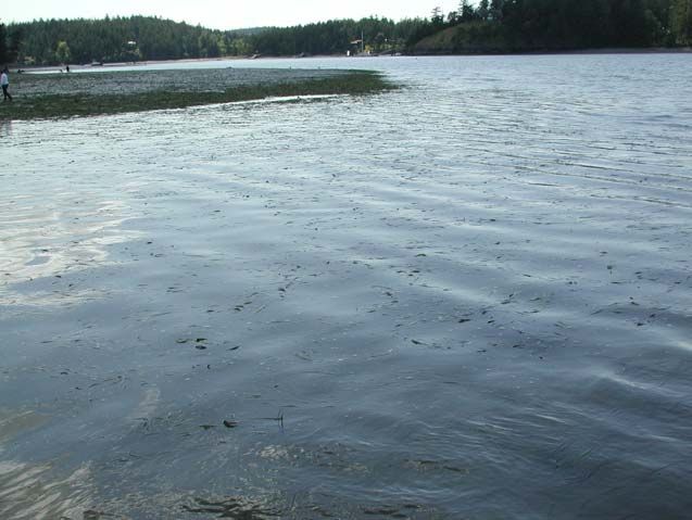

Underwater Light Availability in
                 Westcott Bay
 Analysis of 2007-2008 Data from Three Stations

                                         April 2009

                        by Pete Dowty and Lisa Ferrier
                           Nearshore Habitat Program
                           Aquatic Resources Division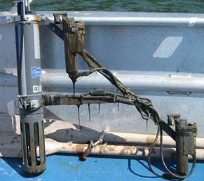
Acknowledgements
Jessie Lacy of the USGS was very helpful with suggestions on data cleanup and
analysis, as well as the deployment of the instruments. Her specific suggestions on
methods for data cleanup, the use of an error analysis and the use of nighttime PAR
are very much appreciated.

The analysis reported here would not have been possible without the work of Anja
Schanz, Jeff Gaeckle and Michael Friese (DNR) and Sandy Wyllie-Echeverria and
Zach Hughes (Seagrass Lab at UW Friday Harbor Labs) who played a key role in
maintaining the field instruments. Jeff Gaeckle also provided underwater
photographs of the instruments.

Discussions with Jim Kaldy (EPA Newport OR), Blaine Kopp (USGS Augusta
ME) and Ken Moore (Virginia Inst. of Marine Science) were very helpful in
interpreting the results and putting them in a broader context of other studies of
seagrass and light. Comments on an earlier draft from Megan Dethier (UW Friday
Harbor Labs) were also very helpful.

Doug Bulthuis and Paula Margerum of the Padilla Bay National Estuarine Research
Reserve were very generous with their time in discussing their deployment and use
of YSI 6600 instruments.

We are grateful to Emily Carrington at UW Friday Harbor Labs, who makes
surface PAR data, as well as other weather variables, available for download over
the internet.

All contributors are DNR staff unless otherwise indicated.
Copies of this report may be obtained from the Nearshore Habitat Program –
Enter seach term ‘nearshore habitat’ on DNR home page: http://www.dnr.wa.gov

ii
Contents
EXECUTIVE SUMMARY ............................................................................................................. 1

1       Introduction ....................................................................................................3

2       Methods ..........................................................................................................5
2.1     Instruments ......................................................................................................5
2.2     Deployment......................................................................................................5
2.3     Data Cleanup ...................................................................................................7
2.4 Assessment of Daily PAR ................................................................................8
2.4.1 Comparison of Daily PAR between Years and Months.................................9
2.4.2 Comparison of Daily PAR between Stations...............................................10
2.5 Calculation of Attenuation ..............................................................................10
2.5.1 Comparison of Daily Attenuation between Years and Months....................11
2.5.2 Comparison of Daily Attenuation between Stations ....................................11

3       Results ..........................................................................................................12
3.1     Data Inventory................................................................................................12
3.2 Daily PAR.......................................................................................................12
3.2.1 Comparison of Daily PAR between Years and between Months ................15
3.2.2 Comparison of Daily PAR between Stations...............................................20
3.3 Attenuation.....................................................................................................24
3.3.1 Comparison of Daily Attenuation between Years and between Months .....24
3.3.2 Comparison of Daily Attenuation between Stations ....................................28

4       Discussion....................................................................................................30
4.1     Does PAR Availability Match the Pattern of Eelgrass Loss? .........................31
4.2     Do Differences between Stations have Physiological Significance? .............33
4.3     Lessons Learned – PAR Data from the YSI 6600 EDS Platform...................35

5       Summary and Recommendations ..............................................................37

6       References....................................................................................................39

APPENDICES
Appendix A PAR Deployment Issues ...............................................................43
A.1  Variation in Deployment Elevation ..............................................................43
A.2  Unattached Sensor .....................................................................................52
A.3  Reversed PAR Connections .......................................................................52

                                                                                                                              iii
A.4       PAR Sensor Error Analysis.........................................................................55
A.5       Correction for Reversed PAR Connections ................................................57
A.6       Out-of-Water Observations.........................................................................58
A.7       References .................................................................................................63
Appendix B PAR Data Cleanup ........................................................................64
B.1  PAR Data Anomalies ..................................................................................64
B.2  Cleanup Algorithm ......................................................................................68
B.3  References .................................................................................................69

iv
EXECUTIVE SUMMARY
The Washington State Department of Natural Resources (DNR) is steward of 2.6
million acres of state-owned aquatic land. DNR manages these aquatic lands for the
benefit of current and future citizens of Washington State. As part of its
stewardship responsibilities, DNR investigates the causes of observed losses in
eelgrass in greater Puget Sound through the Eelgrass Stressor-Response Project.

Eelgrass (Zostera marina) is a flowering aquatic plant that supports nearshore food
webs, provides habitat for many organisms, and is recognized as an indicator of
ecosystem health. DNR has dedicated substantial effort to understanding the
causes of the extensive Z. marina losses in Westcott Bay, San Juan Island.
Westcott Bay was a herring spawning site, and it is one example of a regional
pattern of Z. marina loss in shallow embayments in the San Juan Archipelago.
Several groups are collaboratively investigating the loss, including the University
of Washington Friday Harbor Labs, the USGS Pacific Science Center, Friends of
the San Juans, and DNR. Identifying stressors related to observed Z. marina
declines is an important first step toward formulating management responses to
environmental degradation. Guidance regarding stressors of greatest concern is
needed by multiple efforts to restore and protect Puget Sound, most notably the
regional Puget Sound Partnership’s Action Agenda.

The purpose of the work contained in this report was to quantitatively assess light
limitation as a stressor that reduces the viability of habitat in Westcott Bay for Z.
marina. Field observations of high water column turbidity at the head of Westcott
Bay suggested the possibility that low light transmission through the water column
may have played a role in the loss of Z. marina and continued lack of
recolonization. The specific objectives were to assess two hypotheses related to
light availability, which is measured as photosynthetically active radiation (PAR):
H1: PAR is reduced in areas that have lost Z. marina relative to areas where Z.
    marina persists near the mouth of Westcott Bay at Mosquito Pass.
H2: PAR levels in areas of Z. marina loss are less than the minimum PAR
    requirements reported in the literature for other sites.

To test these hypotheses, YSI instruments with sensors that continuously measure
PAR were deployed at three stations in Westcott Bay in 2007 and 2008.
Monitoring was conducted at the mouth of the bay at Mosquito Pass (station WP)
where Z. marina beds are currently intact; an intermediate location at Bell Point
that has experienced extensive Z. marina loss but supports a small residual bed
(station BP); and the head of the bay where Z. marina has experienced a complete
die-off (stations WBS and WBN).

Executive Summary                                                                       1
Key findings include:
PAR and attenuation observations indicate that PAR at the head of the bay
is reduced relative to other points in the Westcott Bay area. In terms of
mean daily PAR and season cumulative PAR, this reduction at the head of
the bay is roughly 20%.
-2 -1
The reduced average daily PAR at the head of the bay (8.4 mol m day ) is
still nearly threefold greater than the minimum requirements for Z. marina
survival reported for Z. marina beds in Pacific Northwest estuaries (3 mol
m-2 day-1; Thom et al., 2008).
Average daily PAR was indistinguishable between the mouth of the bay
(WP) and Bell Point (BP). Average attenuation was also very similar
between these two stations.
These findings strongly suggest that PAR is not an important controlling factor on
Z. marina abundance in the Westcott Bay area. This conclusion is supported by the
stark differences in Z. marina abundance and survival – Z. marina is abundant at
the mouth of the bay and severely restricted at Bell Point, two sites with
indistinguishable average levels of PAR.
In the course of this study, the Bell Point site emerged as a unique site given that it
has experienced severe loss of Z. marina but still has a small residual bed. This Z.
marina bed has high conservation value due to its rarity within Westcott Bay. It
also provides a unique opportunity for future research to isolate stressors in this
embayment.
This study was the Nearshore Habitat Program’s first effort to deploy unattended
PAR sensors and analyze the resultant datasets. Several methodological
improvements were recommended for future projects, including conducting regular
instrument intercomparisons, migrating to a more advanced analysis platform, and
making the datasets easily available to other researchers.
2 Washington State Department of Natural Resources1 Introduction
Eelgrass (Zostera marina) is a flowering aquatic plant that is common in marine
nearshore subtidal and lower intertidal areas in greater Puget Sound. As a primary
producer, it supports nearshore food webs and provides habitat for many organisms
– including listed salmonids.
The Nearshore Habitat Program (NHP) of the Wash. Department of Natural
Resources (DNR) has documented cases of eelgrass decline in greater Puget Sound
through its annual monitoring project (Gaeckle et al. 2007). DNR initiated the
Eelgrass Stressor-Response Project in 2005 to investigate causes of these declines
(Dowty et al. 2007). Identifying stressors related to observed declines is an
important first step toward formulating management responses to degradation.
Guidance regarding stressors of greatest concern are needed by multiple efforts to
restore and protect Puget Sound, most notably the regional Puget Sound
Partnership’s Action Agenda.
The loss of eelgrass at the head of Westcott Bay on San Juan Island has received
considerable attention because it is a site of total loss and evidence suggests that it
may be one example of a regional pattern of decline in shallow embayments of the
San Juan Islands (Wyllie-Echeverria et al. 2003). Several groups are currently
collaborating on investigations of the eelgrass loss in Westcott Bay including the
University of Washington Friday Harbor Labs, the USGS Pacific Science Center,
Friends of the San Juans, and DNR.
Observations of high turbidity at the head of Westcott Bay in 2006 suggested that
low light transmission through the water column may have played a role in the loss
of eelgrass and continued lack of recolonization (Kevin Britton-Simmons and
Sandy Wyllie-Echeverria, pers. comm.). This report describes the deployment by
DNR of YSI water quality monitoring instruments at three stations in Westcott Bay
from 4/22/07 to 11/2/07 and again from 4/10/08 to 8/8/08. The report focuses only
on the data collected by underwater PAR1 sensors on the YSI instruments. The
purpose of this work was to assess light limitation as a stressor that reduces the
viability of habitat in Westcott Bay for eelgrass.
The objectives of this study were to assess two research hypotheses pertaining to
PAR:
1
Photosynthetically active radiation (PAR), the 0.4 – 0.7 m portion of the solar spectrum.
Introduction 3H1: Reduction of PAR to levels insufficient to support eelgrass survival caused
the loss of eelgrass in Westcott Bay.
H2: Current levels of PAR are insufficient to support eelgrass survival and
prevent eelgrass recolonization in areas of loss.
Only H2 can be directly assessed using current PAR conditions. In the absence of
historical data, at best H1 can be assessed indirerctly, but cannot be formally tested.
To address H2, it was broken down into two testable hypotheses:
HA1: PAR is reduced in areas that have lost eelgrass relative to areas where
eelgrass persists near the mouth of Westcott Bay at Mosquito Pass.
H01: [null] There is no difference in PAR availability between areas that have lost
eelgrass and areas that currently sustain eelgrass in Westcott Bay.
HA2: PAR levels in areas of eelgrass loss are less than the minimum PAR
requirements reported in the literature for other sites.
H02: [null] PAR levels in areas of eelgrass loss are greater or equal to the minimum
PAR requirements reported in the literature for other sites.
These hypotheses do not include specific PAR variables to be tested. Rather, they
were used more generally to guide the analysis presented in this report.
4 Washington State Department of Natural Resources2 Methods 2.1 Instruments The PAR data were collected in Westcott Bay in the San Juan Islands with YSI 6600 EDS instruments with the dual PAR sensor kit offered by YSI. This instrument is unique in that it provides off-the-shelf capability to measure underwater PAR simultaneously at two depths, and the PAR sensors are automatically wiped to minimize biofouling during extended deployments. The PAR sensors used are the Li-Cor LI-192. This configuration with PAR sensors only recently became available. It was developed through YSI collaboration with the Chesapeake Bay National Estuarine Research Reserve (Moore et al. 2004). It has since been deployed in other seagrass systems (Kopp and Neckles 2004). The upper PAR sensor is denoted as the PAR1 sensor and the bottom sensor as PAR2. In addition to the PAR sensors, the instruments used in this study included YSI sensors measuring temperature, conductivity, pH, depth, dissolved oxygen, turbidity and chlorophyll, although data from these sensors are not considered here. Figure 2-1. The YSI 6600 EDS with dual PAR kit (left) and a close-up of the lower PAR sensor and wiper with fouling accumulated over 3 weeks and 4 days in Westcott Bay. 2.2 Deployment The YSI 6600 EDS instruments were deployed at three stations in Westcott Bay over a six-month period in 2007 and a four-month period in 2008. The three 2007 Methods 5
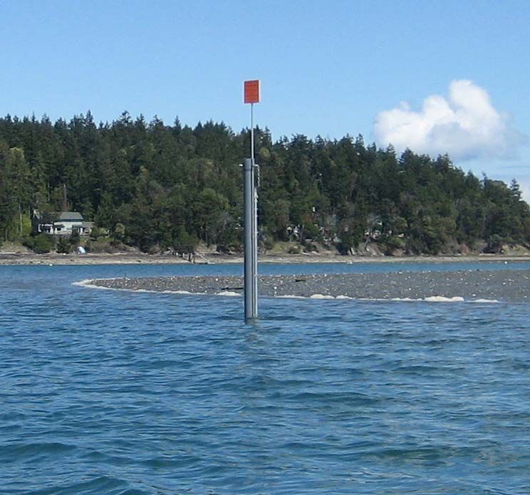
stations are denoted White Point (WP), Bell Point (BP) and Westcott Bay South
(WBS), and their locations are shown in Figure 2-2. In 2008, YSI instruments were
deployed at two stations that had been monitored in 2007 with YSI instruments
(WP and BP), and a third station referred to as Westcott Bay North (WBN). The
stations were selected to characterize a gradient in Z. marina condition as well as
oceanographic and substrate properties (Grossman et al. 2007; Wyllie-Echeverria et
al. 2003). WBS and WBN at the head of the bay have had total die-off of Z.
marina. WP near the mouth at Mosquito Pass has the largest Z. marina bed of the
three stations. BP has an intermediate position and has had significant Z. marina
loss but currently supports a small, residual subtidal bed. The instruments were
placed above sediment at -1.5 m MLLW as determined by the use of tables of
predicted tide and measurements of water depth at the time of deployment. The
instruments were placed vertically so that the lowest sensors on the YSI instrument
were approximately 20 cm above the sediment surface. The lower PAR sensor was
about 10 cm above these lowest sensors, and therefore about 30 cm above the
sediment surface.
Figure 2-2. Map of Westcott Bay area with the locations of the three YSI
deployments in 2007 (WP, BP and WBS) and 2008 (WP, BP and WBN).
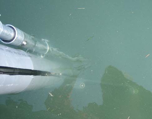
6 Washington State Department of Natural ResourcesThe deployment apparatus was a modified version of the system used at the Padilla Bay National Estuarine Research Reserve. The instrument was lowered through a vertical 6-inch PVC tube to the deployment height. A slot was cut down the length of the tube to accommodate the PAR bracket (Figure 2-3). The PVC tube was attached to galvanized steel conduit that was driven into the sediment to provide support. The positions of the PAR sensors on the PAR brackets were modified after delivery by YSI to allow the instrument to pass through the deployment tube. The vertical separation between the two sensors was 40.5 cm, except for one instrument that had 39.0 cm separation. Figure 2-3. Deployment photos. The instruments were retrieved approximately once a month for cleaning, data download and calibration. There was generally a 1-3 day data gap before the instruments were redeployed, although in one case this data gap reached 5 days. 2.3 Data Cleanup Prior to analysis, the data were passed through several processing steps to address specific deployment issues and unexplained data anomalies. These steps are described in detail in appendices and only summarized here. These initial processing steps led to an adjustment of some data values and elimination of others. Data were adjusted for deployments where PAR1 and PAR2 cables had been reversed (Appendix A.3, p.54). Data were eliminated in one deployment with an unattached and downward facing PAR sensor (Appendix A.2, p.54), and other deployments where PAR wipers were malfunctioning and a clear effect on the data was observed (all such eliminated data indicated in Figure 3-1). Methods 7
Additional data processing addressed patterns in the data that could not be
definitively explained but were considered anomalies. Three unexplained patterns
in the data were identified for cleanup:
Negative attenuation coefficients with values less than could readily be
explained by instrument error;
Significant increments in PAR of opposite sign in the PAR1 and PAR2
sensors from one observation to the next;
Apparent signal loss where there was an abrupt decline in observations of
mid-day PAR to unrealistically low values with little or no variation before
an abrupt return to expected values. During subsequent servicing of the
instruments by YSI to address this issue, intermittent connections within the
PAR electronics were isolated. These connections likely caused the signal
loss observed.
Examples of these unexplained patterns are shown in Figure B-1 (p.68). The cause
of these patterns remains unresolved but likely involves some combination of the
following factors:
Random errors in the Li-Cor sensor due to finite precision. Precision is not
characterized in the Li-Cor literature and was not addressed on the phone by
Li-Cor technical staff. Given the simplicity of the sensor itself, and
segments of uniform data in low-light conditions (Figure B-2, p.69), it
seems unlikely that this plays a significant role.
Problems in the YSI signal processing and logging system. Irregularities in
the low-light data (Figure B-2, p.69) and consultations with other
researchers suggest that this is a possibility with reasonable likelihood.
Sensor obstruction. This could be caused by intermittent covering of the
sensor by plants and algae that are attached to the instrument or deployment
apparatus. It could also be caused by the temporary settling of floating
detritus on the sensor. Given field observations of attached plants and algae
on these instruments, and of floating debris in Westcott Bay, some level of
sensor obstruction is almost certain.
Regardless of the sources of these patterns in the data, they were considered
anomalies and they were removed from the data through the use of a cleanup
algorithm and manual inspection for the signal loss pattern. Bad data points were
removed and were subsequently replaced with linearly interpolated values if (a) no
more than 20% of the daylight data points for the day were bad and (b) there were
no more than two consecutive bad data points. Bad data points that did not meet
these two criteria were replaced with a bad data flag (-9999). Additional details are
described in Appendix section B.2 (p.71).
During the course of the analysis, it became clear that the deployment elevation
varied across stations and even across individual deployments. It is impossible to
fully correct the data for this issue, but the effect on the data was assessed in
Appendix A.1 (p.44).
8 Washington State Department of Natural Resources2.4 Assessment of Daily PAR
Daily PAR is the integral of PAR quanta received on a horizontal surface
throughout the day. It was estimated for stations on days with good PAR data
throughout the daylight hours. Daylight hours were taken to be those between
daily sunrise and sunset at Friday Harbor that was obtained in Pacific Standard
Time from the US Naval Observatory (http://aa.usno.navy.mil/data/docs/RS_OneYear.php).
Daily PAR, Id , was estimated using only daylight PAR measurements as
sec
Id Ii 60 F
min
where the sum is only over daylight hours of individual PAR measurements Ii. The
sampling interval, F, in 2007 was 30 minutes for measurements prior to June 16,
2007 and 15 minutes from June 16 forward. In 2008, the sampling interval was 15
minutes throughout.
2.4.1 Comparison of Daily PAR between Years and Months
To compare available PAR in 2007 to that in 2008, average daily PAR values were
calculated for each day for each station and each sensor (upper and lower). The
overall difference between years was tested for significance with a two-way
ANOVA with year and station as factors. PAR1 and PAR2 results were tested
separately. For this analysis, data from stations WBS (2007) and WBN (2008)
were combined to represent conditions at the head of the bay. Data used in the
ANOVAs were restricted to the sampling period common to both years. These
ANOVAs with unequal replication were run using Statistica (StatSoft Inc.).
Monthly average daily PAR values were also calculated and plotted for each station
and each sensor. The data used to calculate these averages were still restricted to
the sampling period common to both years. Differences in months were tested with
an unequal replication multiple ANOVA with month, year and station as factors
(Statistica, StatSoft Inc.). Again, data from stations WBS (2007) and WBN (2008)
were combined to represent conditions at the head of the bay.
An independent assessment of PAR differences between 2007 and 2008 was
conducted using simulated submarine PAR data based on surface PAR data and
tidal height observations collected at Friday Harbor. Conditions at Friday Harbor
likely diverge somewhat from those at Westcott Bay, being 12 kilometers distant
and on the opposite side of San Juan Island. However, the Friday Harbor data
records benefit from virtually no missing data, and it is reasonable to assume that
any significant differences between years at Friday Harbor would also affect
Westcott Bay.
The Friday Harbor PAR data were obtained from the Carrington Lab at Friday
Harbor Laboratories at a frequency of 15 minutes
(http://depts.washington.edu/fhl/fhl_wx.html). The tidal height observations were
obtained from NOAA at a frequency of one hour (http://tidesandcurrents.noaa.gov,
station 9449880). The tide data were linearly interpolated to 15 minute frequency
Methods 9to match the PAR data. At each 15 minute sample time between 4/1 and 8/31 for
each year, submarine PAR was simulated at a depth of -1.5m MLLW by
calculating the height of the overlying water column (given the tide). The PAR at
depth was then calculated as the residual PAR quantum flux when the incident
surface PAR (from FHL) was attenuated through the water column according to
Beer’s Law with a constant attenuation coefficient of 0.5 m-1. This attenuation is
within the range of mean attenuation observed in Westcott Bay (below). The two
years of simulated submarine PAR were tested for significant difference using a
one-way ANOVA with year as factor, and a two-way ANOVA with year and
month as factors (equal replication ANOVAs conducted with Microsoft Excel).
2.4.2 Comparison of Daily PAR between Stations
To compare available PAR across stations, the mean daily PAR over 2007-2008
was calculated for each station by pooling data from both 2007 and 2008. Only
days with contemporaneous data across the stations were considered. This allowed
for analysis with a repeated measures ANOVA (Microsoft Excel) to test for
significant differences between stations. The Tukey test was used for
multicomparison follow-up tests (Zar 1999, p.210). For this analysis, data from
stations WBS (2007) and WBN (2008) were combined to represent conditions at
the head of the bay.
2.5 Calculation of Attenuation
The simultaneous PAR1 and PAR2 data were used to calculate attenuation for
those observations within three hours of solar noon (i.e. a six-hour window). The
attenuation coefficient was calculated for each observation considered as well as on
a daily basis. Data collected at low sun angles was not considered due to the longer
light path in the water and altered relative path lengths for light reaching the PAR1
and PAR2 sensors. This tends to decrease the apparent attenuation (Carruthers et
al. 2001).
This sun altitude effect is minimal in turbid water, but Kirk (1977, 1984)
recommends restricting measurements to within 2 hours of solar noon in clear
water conditions. Others generally recommend using data within 3 hours of solar
noon, and that was the method used here (Blaine Kopp, USGS Patuxent Wildlife
Research Center, pers. comm.).
The civil time (PDT) of solar noon was estimated on a daily basis as the midpoint
between Friday Harbor sunrise and sunset obtained in PST from the US Naval
Observatory (http://aa.usno.navy.mil/data/docs/RS_OneYear.php).
Attenuation was calculated from Beer’s Law, I 2 I1 e kd , as
k
I
ln I2
1
(Eqn 2-1)
d
Where
k is the attenuation coefficient [m-1]
10 Washington State Department of Natural ResourcesI2 is the PAR irradiance measured by the PAR2 (lower) sensor [mol m-2 s-1],
I1 is the PAR irradiance measured by the PAR1 (upper) sensor [mol m-2 s-1],
d is the vertical distance separating the two sensors [m].
Individual pairs of PAR measurements within the ±3 hour time window around
solar noon were used in Equation 2-1 to calculate attenuation for each sampling
time. These discrete attenuation values were only used as a check on data quality
in the data cleanup process.
2.5.1 Comparison of Daily Attenuation between Years and Months
Daily attenuation was calculated with equation 2-1 using the sum of PAR1 and the
sum of PAR2 within each day’s ±3 hour time window around solar noon (following
Blaine Kopp, pers. comm.). These results were tested for significant differences
between years with an unequal replication two-way ANOVA with year and station
as factors (Statistica, StatSoft Inc.). The data for this analysis were restricted to the
common sampling period between years (4/21 – 8/8).
Monthly and seasonal average attenuation were calculated as simple arithmetic
means of the daily attenuation values. Monthly differences were examined with an
unequal replication multiple ANOVA with month, year and station as factors
(Statistica, StatSoft Inc.). Again, the data were restricted to the common sampling
period (4/21 – 8/8).
2.5.2 Comparison of Daily Attenuation between Stations
Station differences were examined by combining data from 2007 and 2008 and
conducting a repeated measures ANOVA with day and station as factors (Microsoft
Excel). Only days with contemporaneous data across the stations were considered.
The Tukey test was used for multicomparison follow-up tests (Zar 1999, p.210).
For this analysis, data from stations WBS (2007) and WBN (2008) were combined
to represent conditions at the head of the bay.
All confidence intervals presented are based on a t distribution.
Methods 113 Results
3.1 Data Inventory
Figure 3-1 shows the scope of the data collection at the three stations. Data
collection in 2007 started on 4/21/07 and ended on 11/2/07. In 2008, data was
collected from 4/10/08 to 8/8/08. The common period between the two years was
then 4/21 to 8/8. Regular gaps in the data reflect maintenance time for instrument
retrieval, cleaning, data download and calibration. Five different instruments were
used over the entire data collection. The data cleanup reduced the amount of usable
data, particularly for analyses that require contemporaneous data across all three
stations.
1 2 3 4 5 6 7
WBS
1 2 2a 3 4 5 6
2007
BP
no PAR1
2 2a 3 4 5 6 7
WP
4/10 5/1 5/22 6/12 7/3 7/24 8/14 9/4 9/25 10/16 11/6
Instrument Instrument Instrument Instrument Instrument
07C 1026 AB 07C 1387 AB 07C 1387 AA 07C 1026 AC 07C 1276 AA
1 2 3 4
WBN
no PAR1
1 2 3 4
2008
BP
no PAR2 from 6/17
1 2 3 4a 4
WP
no PAR1 from 6/18 no PAR1
4/10 5/1 5/22 6/12 7/3 7/24 8/14 9/4 9/25 10/16 11/6
Figure 3-1. Data coverage in 2007 (top) and 2008 (bottom) using five different YSI 6600 EDS
instruments. Each discrete deployment period was assigned a number that appears above
each bar. Notes under the bars indicate specific deployments where data was removed due to
instrument problems.
3.2 Daily PAR
The daily PAR results are shown in Figure 3-2 and Figure 3-3. The data points
with contemporaneous data across the three stations are distinguished from data
points without corresponding data at the other stations. It is clear that the
12 Washington State Department of Natural Resources35
(a) 2007 daily PAR (PAR1)
30
WP
daily PAR (mol m -2 day -1)
25
BP
WBS
20
15
10
5
0
4/15 4/25 5/5 5/15 5/25 6/4 6/14 6/24 7/4 7/14 7/24 8/3 8/13 8/23 9/2 9/12 9/22 10/2 10/12 10/22 11/1 11/11
35
(b) 2007 daily PAR (PAR2)
30
WP
daily PAR (mol m -2 day -1)
25 BP
WBS
20
15
10
5
0
4/15 4/25 5/5 5/15 5/25 6/4 6/14 6/24 7/4 7/14 7/24 8/3 8/13 8/23 9/2 9/12 9/22 10/2 10/12 10/22 11/1 11/11
Figure 3-2. 2007 daily PAR as estimated by data from the (a) PAR1 and (b) PAR2 sensors at WP, BP and WBS stations. Only days with complete data
between sunrise and sunset are shown and the daily estimates are based on these daylight data only. Days with contemporaneous daily PAR estimates
at all three stations are shown as solid circles. Hollow circles indicate that data are missing for one or both of the other stations for that day (limiting
direct comparisons across stations).
1314
45
(a) 2008 daily PAR (PAR1) WP
40 BP
WBN
35
daily PAR (mol m -2 day -1)
30
25
20
15
10
5
0
4/5 4/15 4/25 5/5 5/15 5/25 6/4 6/14 6/24 7/4 7/14 7/24 8/3 8/13
35
(b) 2008 daily PAR (PAR2) WP
30
BP
WBN
daily PAR (mol m -2 day -1)
25
20
15
10
5
0
4/5 4/15 4/25 5/5 5/15 5/25 6/4 6/14 6/24 7/4 7/14 7/24 8/3 8/13
Figure 3-3. 2008 daily PAR in the same format as Figure 3-2. Note the extended y-axis in (a).contemporaneous data are not uniformly distributed through the data record (see
also Figure 3-5). There is a clear reduction in daily PAR from mid-August through
the end of the 2007 data series for both PAR1 and PAR2 sensors. In 2008 the data
record ends before this reduction would have been observed. The stations at the
head of the bay (WBS and WBN) clearly tend to have lower daily PAR values in
both years.
3.2.1 Comparison of Daily PAR between Years and between Months
Figure 3-4 compares the average daily PAR over the common sampling period
(4/21 – 8/8) between years for each station. The daily PAR data available for these
averages were not uniformly distributed through the common sampling period. For
example, the 2007 data from WP do not include any values from April or early
May (Figure 3-5).
The PAR2 averages are clearly reduced relative to the PAR1 averages. Differences
in average daily PAR between years appear minor relative to the 95% confidence
intervals. This is confirmed by the two-way ANOVA with year and station as
factors which shows no significant effect (=0.05) associated with year (Table
3-1). Differences between stations were significant, but a later test (Table 3-4,
p.20) provides a more robust assessment of differences between stations. This test,
however, is the best single test for differences between years in average daily PAR.
20 20 20
18 WP 18 BP 18
WBS/WBN
16 16 16
daily PAR (mol m day )
-1
14 14 14
-2
12 12 12
2007
10 10 10
2008
8 8 8
6 6 6
4 4 4
2 2 2
0 0 0
PAR1 PAR2 PAR1 PAR2 PAR1 PAR2
Figure 3-4. Comparison of average daily PAR across years. Daily PAR was averaged only
over the period that was sampled in both years (April 21 – August 8). The distribution of data
with each year varies across the stations, so differences between stations should be interpreted
cautiously (see Figure 3-5) Error bars are 95% confidence intervals on the means. Sample
sizes range from 41 to 94 days for the averages.
Results 15WP
April May June July August September October
2008
PAR2
2007
2008
PAR1
2007
BP
April May June July August September October
2008
PAR2
2007
2008
PAR1
2007
WBS/WBN
April May June July August September October
2008
PAR2
2007
2008
PAR1
2007
Figure 3-5. The distribution of daily PAR data available for analysis. The red boxes delineate
the dates of sampling that were common to 2007 and 2008, April 1 to August 8.
Source of Variation SS df MS F P-value
PAR1 ANOVA Year 70.6 1 70.6 1.255 0.263311
Station 1110.3 2 555.1 9.873 0.000065
Interaction 3.4 2 1.7 0.030 0.970108
Within 23279.2 414 56.2
PAR2 ANOVA Year 55.11 1 55.11 1.796 0.180897
Station 771.36 2 385.68 12.569 0.000005
Interaction 9.67 2 4.84 0.158 0.854222
Within 13379.2 436 30.69
Table 3-1. ANOVA tables testing for significant differences (=0.05) in average daily PAR
between years and between stations. The data are restricted to days with contemporaneous
data across stations in the 4/21 – 8/8 period. The data are summarized in Figure 3-4. PAR1
(top) and PAR2 (bottom) data were analyzed separately.
There were also no obvious differences between years in monthly average daily
PAR (Figure 3-6). These results should be interpreted with caution given some
relatively low sample sizes and the particularly poor representation of the months
of August (8/1 – 8/8) and April (4/21 – 4/30). Month did not have a significant
effect in a multiple ANOVA (not shown) with month, year and station as factors
for either the PAR1 or PAR2 analysis. To ensure reasonable coverage across all
three stations, this analysis was restricted to May-June for PAR1 and May-June-
July for PAR2. The station factor was significant for both PAR1 and PAR2, and
the month-year-station interactions were significant in the PAR2 analysis.
16 Washington State Department of Natural ResourcesPAR1 PAR2
30 30
9 19 11 18 26 27
25 2007 P1
25
2008 P1 20 18 23 27 6
20
-1
20
mol m day
WP
15 -2 15
10 10
20 19 12 27
5 5 2007 P2
10 25 16 20 26 2008 P2
0 0
Apr May Jun Jul Aug Sep Oct Apr May Jun Jul Aug Sep Oct
30 30
2007 P1 9 22 13 16 27 27
25 25
2008 P1
19 21 9 21 6
20 20
-1
mol m day
BP
15 15
-2
10 10
20 24 24 24 7
5 5 2007 P2
9 24 4 20 27 27 2008 P2
0 0
Apr May Jun Jul Aug Sep Oct Apr May Jun Jul Aug Sep Oct
30 30
23 24 26 7 10 20 27 25 22 27 28
25 25
WBS/WBN
10 21 27 25 23 27 28 20 27 24 26 7
20 20
-1
mol m day
2007 P1
15 15
-2
2008 P1
10 10
5 2007 P1 5
2008 P1
0 0
Apr May Jun Jul Aug Sep Oct Apr May Jun Jul Aug Sep Oct
Figure 3-6. Comparison between 2007 and 2008 of monthly averages of daily PAR. Error bars
are 95% confidence intervals. All available data were used to compute these averages. These
values therefore do not represent the input data to the ANOVA in Table 3-1, which was a subset of
the data shown here. Blue numbers represent sample sizes (number of values of daily PAR) for
the 2007 monthly averages, and pink numbers represent samples sizes for the 2008 monthly
averages. (P1 = PAR1; P2 = PAR2). Note the small sample sizes for the August 2008 averages.
The simulated submarine PAR results for Friday Harbor are shown in Figure 3-7.
While there are intervals with apparent differences between the years (e.g. lower
July PAR in 2007), there is high variability within each year, and in the difference
between the years. The monthly means of the simulated daily PAR at Friday
Harbor are shown in Figure 3-8.
Results 1718
40
PAR
0
-40
60
2007
50 2008
daily PAR (mol m -2 day -1)
40
30
20
10
0
4/1 4/11 4/21 5/1 5/11 5/21 5/31 6/10 6/20 6/30 7/10 7/20 7/30 8/9 8/19 8/29
Figure 3-7. Daily PAR simulated for -1.5 m MLLW at Friday Harbor from 4/1 to 8/31. The top graph shows the corresponding PAR difference
(2008 minus 2007) between the two years (also in mol m-2 s-1).40
35
daily PAR (mol m -2 day -1)
30
2007
2008
25
20
15
Ap My Jn Jl Au
Figure 3-8. Monthly average of daily simulated PAR at -1.5m MLLW depth at Friday
Harbor. Error bars are 95% confidence intervals.
The one-way ANOVA with year as the factor did not detect a significant difference
between 2007 and 2008 Friday Harbor simulated daily PAR (Table 3-2). The two-
way ANOVA with year and month as factors supported the following points (Table
3-3):
There is significant variation in daily PAR by month.
There is no significant difference between years.
There is no significant interaction. This means that the same month effect
is seen in both years.
Source of Variation SS df MS F P-value
Between Groups 9.699709 1 9.699709 0.088764 0.765958
Within Groups 33219.83 304 109.2758
Table 3-2. One-way ANOVA table testing for significant difference
(=0.05) between 2007 and 2008 simulated daily PAR at Friday
Harbor.
Source of Variation SS df MS F P-value
Months 2317.388 4 579.347 5.672371 0.000208
Year 6.649575 1 6.649575 0.065106 0.798782
Interaction 636.1064 4 159.0266 1.557025 0.185868
Within 29619.12 290 102.1349
Table 3-3. Two-way ANOVA table testing for significant effects
(=0.05) by month and by year, and for significant interactions
between the two, in simulated daily PAR at Friday Harbor.
Results 193.2.2 Comparison of Daily PAR between Stations
The ANOVA that tested for significant differences in mean daily PAR between
years (Table 3-1, p.16), included station as a second factor. The differences
between stations were found to be very significant. An additional ANOVA is
presented here that focuses only on differences between stations. This test benefits
from greater accuracy since input data is limited to only days with
contemporaneous data across all three stations. Furthermore, the two years are
pooled, increasing sample sizes, and for each day, the data from the three stations
are “paired” in a repeated measures design. The results confirm that differences
between stations are highly significant (Table 3-4).
Source of
SS df MS F P-value
Variation
PAR1 ANOVA Day 18273.78 86 212.4858 46.1451 0.000000
Station 396.8206 2 198.4103 43.08836 0.000000
Error 792.0138 172 4.604732
PAR2 ANOVA Day 10917.15 127 85.961807 22.12952 0.000000
Station 636.3375 2 318.16877 81.90757 0.000000
Error 986.6593 254 3.8844854
Table 3-4. Repeated measures ANOVA tables testing for significant differences (=0.05)
between stations in average daily PAR. All days (2007 and 2008) with contemporaneous data
across the three stations were included in the analyses. These ANOVAs were run as two-way
ANOVAs without replication with day and station as factors
The ANOVAs were followed up with Tukey tests to determine which specific
station differences were significant (Zar 1999, p.210). These results show that all
stations were significantly different in terms of daily PAR as measured by the
PAR1 sensors. As measured by the PAR2 sensors, the head of the bay (WBS and
WBN) was significantly different, but WP and BP could not be distinguished. The
2007-2008 average daily PAR values are shown in Figure 3-9.
Station comparison PAR1 results PAR2 results
WP vs WBS/WBN Reject H0 Reject H0
BP vs. WBS/WBN Reject H0 Reject H0
WP vs BP Reject H0 Accept H0
Table 3-5. Results of Tukey mulicomparison tests in follow-up to the
significant ANOVA results (Table 3-4). In each case, the null
hypothesis tested, H0, states that average daily PAR was equivalent
at the two stations tested. All tests performed at =0.05.
It is important to note that these results are based on the assumption of identical
instrument deployment depths at each station. During data analysis, it became
clear that there were depth discrepancies that could affect a comparison of PAR
across stations. It is not possible to accurately correct for the depth discrepancies
with the available information. However, a rough assessment of the effects of the
20 Washington State Department of Natural Resourcesdepth discrepancies on the PAR results is given in Appendix section A.1 (p.44).
This assessment suggests that PAR may have been underestimated at WP.
Furthermore, the significant difference between average daily PAR at WP and BP
measured by the PAR1 sensors (Table 3-5), may be an artifact of the differences in
deployment depth.
18
16
daily PAR (mol m day ) 14
-1
12
-2
10
PAR1
PAR2
8
6
4
2
0
WP BP WBS/WBN
Figure 3-9. Average 2007-2008 daily PAR for the Westcott Bay stations for
each PAR sensor. Only days with contemporaneous data across the stations
were included in the averages (nPAR1 = 87; nPAR2 = 129). Error bars are 95%
confidence intervals.
Cumulative daily PAR provides an alternate approach to reducing the daily PAR
data for simple station comparisons. Figure 3-10 shows the cumulative PAR
separately for data from PAR1 and PAR2 sensors, based on contemporaneous data
across the three stations. In both cases, the seasonal cumulative PAR at the head of
the bay (WBS/WBN) is substantially lower than WP and BP. Based on the PAR1
data, the seasonal cumulative PAR at the head of the bay was reduced in both years
by 17% relative to the next station (WP for both years). Based on the PAR2 data,
cumulative PAR at the head of the bay was reduced by 27% in 2007 (WBS) and
23% in 2008 (WBN) relative to the next station (also WP).
Results 21800
(a) cumulative PAR (PAR1 sensors)
700
600
cumulative PAR (mol m -2)
500
WP
400
BP
WBS
300
200
100
0
5/20 5/30 6/9 6/19 6/29 7/9 7/19 7/29 8/8 8/18 8/28 9/7 9/17 9/27 10/7
600
(b) cumulative PAR (PAR2 sensors)
500
cumulative PAR (mol m -2)
400
WP
300 BP
WBS
200
100
0
5/20 5/30 6/9 6/19 6/29 7/9 7/19 7/29 8/8 8/18 8/28 9/7 9/17 9/27 10/7
Figure 3-10. 2007 cumulative daily PAR based only on contemporaneous daily PAR estimates
at the three stations.
22 Washington State Department of Natural Resources600
(a) cumulative PAR (PAR1 sensors)
500
cumulative PAR (mol m -2)
400
WP
300 BP
WBN
200
100
0
4/10 4/20 4/30 5/10 5/20 5/30 6/9 6/19
600
(b) cumulative PAR (PAR2 sensors)
500
cumulative PAR (mol m -2)
400
WP
BP
300 WBN
200
100
0
4/10 4/20 4/30 5/10 5/20 5/30 6/9 6/19
Figure 3-11. 2008 cumulative daily PAR based only on contemporaneous daily PAR estimates
at the three stations.
Results 233.3 Attenuation
The daily attenuation time series are shown in Figure 3-12. The high values at BP
in 2008 are likely due to bad PAR2 data that was not identified by the cleanup
algorithm. Figure 3-13 gives an example of suspicious PAR2 associated with one
of these spikes in daily attenuation. Five data points shown with high values were
removed from the dataset and not included in the following analyses.
3.3.1 Comparison of Daily Attenuation between Years and between Months
A comparison of the 2007 and 2008 season means of daily attenuation are shown in
Figure 3-14. There is no obvious difference between the years. The estimate for
BP is greater in 2008, but the estimate for WP is lower in 2008 and there is
virtually no difference between years at WBS/WBN. This is supported by the two-
way ANOVA results which show that year is not a significant factor ( = 0.05),
while station is a significant factor. These estimates could reflect a slight bias
associated with seasonality since they are based on different distributions of data
through the common sampling period of April 21 to August 8 (see Figure 3-5,
p.16).
Source of Variation SS df MS F P-value
Year 0.0014 1 0.0014 0.022 0.882460
Station 7.0973 2 3.5487 54.449 0.000000
Interaction 0.3151 2 0.1575 2.417 0.090278
Within 31.0226 476 0.0652
Table 3-6. ANOVA results testing for significant differences in mean daily
attenuation between years and between stations.
Estimates of monthly mean attenuation are shown in Figure 3-15. These values
were calculated as the arithmetic mean of all daily attenuation values for each
month for each station. Comparisons across years are difficult because of the
incomplete monthly data series, but two patterns are consistent across plots in
Figure 3-15:
Estimates of May attenuation were greater in 2007 than 2008 across all
three stations, although these differences have not been formally tested and
the significance of the BP difference is in doubt.
Estimates of June and July attenuation were lower in 2007 than 2008 at BP
and the head of the bay (WBS / WBN). Missing data prevented this
comparison at WP.
24 Washington State Department of Natural Resources2.00
2007 WP
1.75
BP
1.50 WBS
1.25
attenuation (m -1)
1.00
0.75
0.50
0.25
0.00
-0.25
4/15 4/25 5/5 5/15 5/25 6/4 6/14 6/24 7/4 7/14 7/24 8/3 8/13 8/23 9/2 9/12 9/22 10/2 10/12 10/22 11/1
2.00
2008 WP
1.75
BP
1.50 WBN
1.25
attenuation (m -1)
1.00
0.75
0.50
0.25
0.00
-0.25
4/5 4/10 4/15 4/20 4/25 4/30 5/5 5/10 5/15 5/20 5/25 5/30 6/4 6/9 6/14 6/19 6/24 6/29 7/4 7/9 7/14 7/19 7/24 7/29 8/3 8/8 8/13
Figure 3-12. 2007 (top) and 2008 (bottom) daily attenuation coefficient.
251200
PAR1
PAR2
1000
800
PAR ( mol m-2 s-1)
600
400
200
0
5:00 7:00 9:00 11:00 13:00 15:00 17:00 19:00 21:00
Figure 3-13. PAR data from 26 May 2008. The daily attenuation
coefficient based on these data is k=5 m-1, and is off the chart shown in
Figure 3-12. The PAR2 data suggests that that sensor was obstructed,
resulting in unreliable PAR data and daily attenuation estimate.
0.8 0.8 0.8
0.7 0.7 0.7
0.6 0.6 0.6
attenuation (m )
-1
2007
0.5 0.5 0.5
2008
0.4 0.4 0.4
0.3 0.3 0.3
0.2 0.2 0.2
0.1 0.1 0.1
0.0 0.0 0.0
WP BP WBS / WBN
WBSN
Figure 3-14. Comparison of average daily attenuation coefficients calculated for 2007
and 2008. Daily attenuation values were averaged only over the period that was
sampled in both years (April 21 – August 8). Error bars are 95% confidence
intervals. The sample sizes for these six averages range from 55 to 102 daily
attenuation values. These represent the same data that were tested in the ANOVA in
Table 3-6, that showed that the station has a significant effect on the averages. The
year did not have a significant effect.
26 Washington State Department of Natural Resources1
0.9
0.8
WP
attenuation (m -1) 0.7
0.6
2007
0.5
2008
0.4
0.3
29
0.2
11 30 28 28 28
0.1
21 21 13
0
Apr May Jun Jul Aug Sep Oct
1
0.9
0.8
BP
attenuation (m -1)
0.7
0.6
2007
0.5
2008
0.4
0.3
0.2
10 26 15 29 28 28
0.1
21 23 14 28 7
0
Apr May Jun Jul Aug Sep Oct
1
0.9
0.8
WBS / WBN
attenuation (m -1)
0.7
0.6
2007
0.5
2008
0.4
0.3
0.2
10 26 29 29 24 28 29
0.1
25 28 29 7
0
Apr May Jun Jul Aug Sep Oct
Figure 3-15. Mean monthly attenuation calculated as the arithmetic mean of all available
daily attenuation values. Error bars are 95% confidence intervals on the means. Blue
numbers represent sample sizes (number of values of daily attenuation) for the 2007 monthly
averages, and pink numbers represent samples sizes for the 2008 monthly averages. Note the
small sample sizes for the August 2008 averages.
Results 273.3.2 Comparison of Daily Attenuation between Stations
The ANOVA that tested for significant differences in mean daily attenuation
between years (Table 3-6, p.24) included station as a second factor. The
differences between stations were found to be very significant. An additional
ANOVA is presented here that focuses only on differences between stations. This
test benefits from greater accuracy since input data is limited to only days with
contemporaneous data across all three stations. Furthermore, the two years are
pooled, increasing sample sizes, and for each day, the data from the three stations
are “paired” in a repeated measures design. The results confirm that differences
between stations are highly significant (Table 3-7).
Source of Variation SS df MS F P-value
Day 16.979 137 0.123934 2.370429 0.000000
Station 6.136467 2 3.068233 58.68456 0.000000
Error 14.32567 274 0.052283
Table 3-7. Repeated measures ANOVA tables testing for significant differences
(=0.05) between stations in average daily attenuation. All days (2007 and
2008) with contemporaneous data across the three stations were included in the
analyses.
The ANOVA was followed up with Tukey’s test to determine which specific
station differences were significant (Zar 1999, p.210). These results show that all
stations were significantly different in terms of average daily attenuation (Table
3-8). The 2007-2008 average daily attenuation values are shown in Figure 3-16.
Station comparison Attenuation results
WP vs WBS/WBN Reject H0
BP vs. WBS/WBN Reject H0
WP vs BP Reject H0
Table 3-8. Results of Tukey mulicomparison tests in follow-up to the
significant ANOVA results (Table 3-7). In each case, the null
hypothesis tested, H0, states that average daily attenuation was
equivalent at the two stations tested. All tests performed at =0.05.
28 Washington State Department of Natural Resources0.8
0.7
0.6
attenuation (m )
-1
0.5
0.4
0.3
0.2
0.1
0
WP BP WBS/WBN
Figure 3-16. Average 2007-2008 daily attenuation. Only days
with contemporaneous data across the stations were included in
the averages (n=138 days). Error bars are 95% confidence
intervals. The average attenuation for each station is
significantly different than the others (Table 3-8).
Results 294 Discussion
The PAR results are supported by the attenuation results, and they both lead to the
following characterization of PAR across the Westcott Bay stations (Table 4-1):
Average levels of PAR at the head of the bay (WBS / WBN) are reduced
relative to other areas of the bay (both BP and WP stations). The magnitude
of this reduction is roughly 20% as measured by mean daily PAR and
cumulative PAR. Average water column attenuation is increased at the
head of the bay.
Average levels of PAR at BP and WP are very similar. Average attenuation
is very similar between BP and WP.
WP BP WBS / WBN
-2 -1
Average daily PAR (mol m day )
(PAR2 sensor; Figure 3-9, p.21; compare to depth- 11.1 ± 1.0 11.2 ± 1.0 8.4 ± 0.9 *
adjusted results in Figure A-8, p.52)
Average attenuation (m-1)
0.39 ± 0.05* 0.44 ± 0.05* 0.67 ± 0.04 *
(Figure 3-16, p.29)
Table 4-1. Summary of average 2007-2008 PAR and attenuation results (* = significantly
different from other stations, =0.05).
The PAR and attenuation parameters are subject to different limitations. The PAR
parameters provide the most direct measure of the environmental variable of
interest – levels of PAR that would be available to an eelgrass plant at a given
location. However, measurements of PAR are very sensitive to depth of
deployment. Therefore, the strength of comparisons of PAR across stations rests
on tight control of instrument deployment depth. It is very difficult to control
deployment depth to within centimeters in a soft sediment nearshore environment.
An analysis of depth data across the stations in this study showed that depth
discrepancies were large enough to compromise the ability to discriminate between
stations with similar PAR results (WP and BP; Appendix A.1).
In contrast, attenuation results are relatively insensitive to modest differences in
deployment depth since attenuation is based on the difference in readings between
two sensors with a fixed height difference. Where deployment depth problems are
suspected, it is useful to consider attenuation results for this reason. However,
attenuation is only indirectly related to the environmental variable of interest (PAR
30 Washington State Department of Natural Resourcesincident on eelgrass leaves). Furthermore, attenuation was measured over only a
portion of the water column (40 vertical cm) which, depending on vertical
structure, may be a poor representation of the entire water column.
The fact that both the PAR results and the attenuation results are consistent
increases our confidence in the overall characterization. We can now revisit our
initial hypotheses.
4.1 Does PAR Availability Match the Pattern of Eelgrass Loss?
Let us start with the finding that PAR is reduced at the head of the bay where
eelgrass has completely disappeared. By itself, this suggests that the pattern of
available PAR matches the pattern of eelgrass loss. However, when we also
consider the findings at BP, this relationship no longer holds.
BP can be considered to be an intermediate location in terms of current eelgrass
abundance because there is a small, residual sub-tidal bed north of the YSI station
and to the south there is some surviving eelgrass, albeit very sparse (Figure 4-3).
But in general the eelgrass abundance is very low and this station is more similar to
the head of the bay than to WP in terms of current eelgrass condition. During the
fieldwork there was no eelgrass in the immediate vicinity of the BP YSI
instrument, and only one plant was observed in an area of at roughly 200 m2 around
the instrument. Furthermore, when put in a longer temporal context, the Bell Point
area in general must be placed in a category of extreme eelgrass loss. Extensive
beds in the intertidal and subtidal have been lost (Figure 4-1).
Figure 4-1. 2003 photo from the east side of Bell Point looking west. Extensive
eelgrass is visible throughout the foreground up to the lower zone of the
exposed shoreline in the background. Eelgrass has completely disappeared
from these areas. The residual subtidal bed would be underwater to the right
of the exposed point.
Discussion 31The fact that BP and WP have essentially indistinguishable levels of PAR, but very
different levels of current eelgrass abundance (as well as recent trajectories in
abundance), leaves us unable to reject the null hypothesis presented on page 4:
H01: There is no difference in PAR availability between areas that have lost
eelgrass and areas that currently sustain eelgrass in Westcott Bay.
The lack of a relationship between PAR and eelgrass abundance is shown in Figure
4-2. Clearly, if only WP and WBS/WBN were compared, a different conclusion
would be reached – i.e. PAR would seem to predict eelgrass abundance. It is
essentially the BP data point that precludes us from rejecting the null hypothesis.
WP
intact
eelgrass
eelgrass survival
eelgrass
loss
WBS/ BP
WBN
low high
PAR PAR
PAR
Figure 4-2. Conceptual representation of the three stations placed in a space of eelgrass
survival and PAR availability. Under the hypothesis of low PAR-induced eelgrass loss,
prior to 2003 all stations were in the position of WP – i.e. intact eelgrass with high levels of
PAR. The arrows represent trajectories over time as WBS/WBN and BP experienced
extreme loss of eelgrass. PAR does not explain the change in eelgrass survival in these two
trajectories, undermining this hypothesis.
This conclusion is vulnerable to an argument that different stressors may be acting
at different locations in the Westcott Bay area. The analysis would then be
confounded by considering all three stations as representing a single population.
This may be true to some extent, but when the area is considered more synoptically
it seems reasonable to assume there is some shared mechanism behind the loss of
eelgrass across Westcott and Garrison bays. Figure 4-3 shows that eelgrass loss is
complete across the inner bays and persists only in close proximity to the mouth at
Mosquito Pass. Although not shown, eelgrass persists and is abundant at the mouth
and outside the bay in areas of Mosquito Pass. While not definitive, the
32 Washington State Department of Natural ResourcesYou can also read