Road Traffic Forecasts 2018 - Moving Britain Ahead
←
→
Page content transcription
If your browser does not render page correctly, please read the page content below
Road Traffic Forecasts
                 2018

         Moving Britain Ahead

                     July 2018
The Department for Transport has actively considered the needs of blind and partially
sighted people in accessing this document. The text will be made available in full on the
Department’s website. The text may be freely downloaded and translated by individuals or
organisations for conversion into other accessible formats. If you have other needs in this
regard please contact the Department.

Department for Transport
Great Minster House
33 Horseferry Road
London SW1P 4DR
Telephone 0300 330 3000
Website www.gov.uk/dft
General enquiries: https://forms.dft.gov.uk

© Crown copyright 2018
Copyright in the typographical arrangement rests with the Crown.

You may re-use this information (not including logos or third-party material) free of charge
in any format or medium, under the terms of the Open Government Licence. To view this
licence, visit http://www.nationalarchives.gov.uk/doc/open-government-licence/version/3/
or write to the Information Policy Team, The National Archives, Kew, London TW9 4DU, or
e-mail: psi@nationalarchives.gsi.gov.uk

Where we have identified any third-party copyright information you will need to obtain
permission from the copyright holders concerned.
Contents

Executive Summary                                                            5
    Introduction                                                             5
    Improvements to the Forecasts                                            5
    What the Forecasts Show                                                  6
    Forecast Performance & Next Steps                                        7
1. Introduction, Use of Forecasts & How the Model Works                     10
    Introduction                                                            10
    Use of the Forecasts                                                    11
    How the NTM Works                                                       12
    HGV & LGV Forecasting                                                   14
    Public Transport & Active Modes                                         14
    NTM Recalibration & Update                                              14
    Future Development of NTM                                               15
    NTEM7.2 Update                                                          16
2. Evaluating Past Performance                                              18
    Background                                                              18
    Summary of Results                                                      20
    Implications of Results                                                 25
3. Scenarios - Uncertainty and the Drivers of Demand                        27
    Introduction                                                            27
    Reference (Scenario 1) - Context, Assumptions & Inputs                  30
    High GDP, Low Fuel & Low GDP, High Fuel (Scenarios 2 & 3) – Context,
    Assumptions & Inputs                                                 31
    High Migration & Low Migration (Scenarios 4 & 5) – Context, Assumptions &
    Inputs                                                                  35
    Extrapolated Trip Rates (Scenario 6) – Context, Assumptions & Inputs    38
    Shift to Zero Emission Vehicles (ZEVs) (Scenario 7) – Context, Assumptions
    & Inputs                                                                 42
    Trips (All Scenarios)                                                   43
    Car Ownership (All Scenarios)                                           45

                                      3
4. Summary of Results                                 48
    Summary                                           48
    What Drives the Growth?                           48
    Comparisons with RTF15                            50
    Results                                           51
    Traffic                                           51
    Vehicle Type                                      53
    Road Type                                         57
    Region                                            60
    Congestion                                        62
    Emissions                                         68
5. Transport Technology                               74
    Introduction                                      74
    Possible Impacts                                  76
    Demand Sensitivity Tests                          80
    Supply Sensitivity Tests                          87
    Conclusions and Next Steps for Technology Tests   89
6. Summary & Next Steps                               91
    Summary                                           91
    Next Steps                                        92
Annex: Speed Flow Curves                              94
Annex: Glossary of Terms and Acronyms                 98

                                    4
Executive Summary

          Introduction

1         Road Traffic Forecasts 2018 (RTF18) present the latest forecasts for traffic demand,
          congestion and emissions in England and Wales up to the year 2050. These are
          produced using the Department for Transport’s National Transport Model (NTM).
2         The forecasts provide the Department’s strategic view of future road travel demand
          under a number of plausible scenarios that reflect the uncertainty in the key drivers of
          road traffic demand. The forecasts have been disaggregated by vehicle type, road
          type and region and are presented in this document, accompanying spreadsheets
          and in the interactive Road Traffic Forecasts 2018 Visualisation Tool1.
3         This publication follows a substantial update to our modelling suite since Road Traffic
          Forecasts 2015 (RTF15), with a recalibration of the NTM to a new base year of 2015
          and an updated National Trip End Model (NTEM) extending the forecast horizon to
          2050.
4         Understanding future demand for road travel is essential to shape the policies we
          implement and the investments we make. However, forecasting future demand is
          complex and there is significant uncertainty about the extent to which existing trends
          and relationships will carry on into the future. We need to ensure that we understand
          and communicate this uncertainty.
5         Within these forecasts, a scenarios approach has been taken to construct a number
          of different plausible future outcomes. This provides a strategic view of key
          uncertainties that might impact on future road traffic and supports the design of
          strategies and policies that are resilient to these uncertainties.
6         These forecasts are not definitive predictions about the future, or desired futures, but
          show how demand for road travel may evolve assuming no change in government
          policy beyond that already announced. These forecasts have been produced using a
          broad range of research, evidence and data focusing on:
          •     Our understanding of how people make travel choices
          •     The possible paths of key drivers of travel demand

          Improvements to the Forecasts

7         The NTM has been updated to take into account the most recent traffic data and
          trends in travel behaviour. The update rebases the model from 2003 to 2015,
          requiring a full recalibration, and takes all relevant up-to-date evidence and input
          data, whilst retaining the same functionality as the previous model.

1
    http://maps.dft.gov.uk/rtf18-vis

                                                   5
8    Since the publication of our last forecasts in RTF15, we have also comprehensively
     updated the National Trip End Model (NTEM) to reflect more recent evidence. NTEM
     brings together exogenous projections of population, employment and housing
     supply and combines these with projections of car ownership and trip rates to
     forecast future numbers of trips by person type at a detailed spatial level.
9    In preparing RTF18 we have developed a new set of scenarios which aim to improve
     on RTF15 by considering a wider variety of uncertainty and combining multiple
     issues to create plausible future states of the world.
10   As part of this process we have reviewed the evidence on road demand and the
     uncertainty around a number of key drivers of road traffic, including:
     •   Population growth
     •   Trip rates
     •   GDP & Income
     •   Costs of driving
     •   Young people’s driving patterns and licence holding
     •   Demand for goods: freight
     •   Technology
11   After assessing the uncertainty around these key drivers of demand, we have
     combined assumptions related to these issues where possible to create a set of
     seven plausible, internally consistent scenarios. Further discussion of these
     scenarios is set out in section 3.
12   Finally we have developed an interactive visualisation tool to allow users to easily
     navigate through our model outputs and fully explore the forecast results. This can be
     found at http://maps.dft.gov.uk/rtf18-vis

     What the Forecasts Show

13   Traffic in England and Wales is forecast to increase across all scenarios, but the size
     of that growth depends on the assumptions made about the key drivers of future road
     demand. From 2015 traffic is forecast to grow by between 17% and 51% by 2050.
14   The growth in traffic levels is predominately driven by the projected growth in
     population levels (and thus the number of trips) and changes to vehicle running
     costs. Extrapolated Trip Rates (scenario 6), which explores the impacts of
     extrapolating recent trip rate trends, has the lowest forecast growth of 17% by 2050.
15   Traffic growth on the Strategic Road Network (SRN) is forecast to be strong and
     positive in all scenarios, ranging between growth of 32% and 66% by 2050, driven by
     forecast increases in the number of car trips and trip distances, as well as increasing
     Light Goods Vehicle (LGV) traffic. Forecast growth on principal roads and minor
     roads is lower than the SRN, between 10%-47% and 11%-50% respectively.
16   Car traffic is forecast to grow between 11% and 48% by 2050, whilst LGV traffic is
     forecast to continue growing significantly in all scenarios (between 23% and 108%).
     Strong LGV traffic growth has a significant impact on total traffic growth, particularly
     in Extrapolated Trip Rates (scenario 6). In this scenario although car traffic is forecast
     to grow by just 11%, overall traffic growth still reaches 17% with LGV traffic
     accounting for 19% of total traffic. HGV traffic growth is forecast to be lower than
                                              6
other vehicle types, with growth ranging from 5% to 12% by 2050.
17   Congestion is forecast to grow as a result of increases in traffic. The proportion of
     traffic in congested conditions in 2050 is forecast to range from 8% to 16%
     depending on the scenario, compared to 7% in 2015. The average speed during all
     periods is forecast to fall from 34mph in 2015 to as low as 31mph in 2050 in Shift to
     ZEVs (scenario 7). The average delay per vehicle mile during all periods is forecast
     to increase by up to approximately 11 seconds per mile (69%) by 2050, although
     Extrapolated Trip Rates (scenario 6) specifically sees smaller increases (5%).
18   There is great uncertainty around the possible impact of transport technology on road
     traffic demand and it is unclear how far our existing understanding of the drivers of
     demand will continue to apply. In an attempt to address this, we have undertaken
     some initial exploratory analysis of how the introduction of Connected Autonomous
     Vehicles (CAVs) may impact on demand through examining levers in existing
     models. The purpose of the analysis presented is not to make forecasts about how
     CAVs will impact on demand, but to better understand which aspects of these new
     technologies traffic levels might be most sensitive to, thus informing future research
     priorities. The range of traffic growth by 2050 in these tests is between 5% and 71%
     driven principally by uncertainty around possible changes to car occupancy levels,
     alongside possible changes to the perceived values of time and mobility.

     Forecast Performance & Next Steps

19   We have reviewed the performance of RTF15 and the findings emphasise:
     •   that the forecasts performed well at the aggregate level
     •   the importance of keeping the base year and assumptions up-to-date
     •   the amount of uncertainty around road traffic demand (even in the short term).
     •   that the model is likely to overstate the level of traffic growth in London.
20   Important elements to note given this:
     •   The base year of the NTM has been updated to 2015 for RTF18.
     •   In RTF18 we have reflected a broader range of factors in our scenarios, including
         exploring the possible impacts of changes to population levels.
     •   The NTM is a national strategic transport model and therefore has difficulties
         replicating travel patterns at local levels where travel behaviour is substantially
         different from the national picture. This is particularly apparent in London where
         the relationship between income and car ownership differs. Whilst this is a known
         feature of the NTM and is not considered to have a material impact on the
         performance of our forecasts at the national level, it should be considered if
         looking at London outputs.
21   We recognise that our understanding of the drivers of road traffic demand continue to
     evolve and there is uncertainty around travel behaviour. We will continue to work on
     developing the evidence base and forecasting approach to improve the transparency
     and robustness of our strategic modelling capability.
22   Whilst we believe the technology-focused tests have explored some key features of
     CAVs that may impact road traffic demand in the future, these developments present
     a significant challenge to any forecasting activity. We shall explore ways in which
     models may be used more effectively to forecast the impacts in more detail.
                                               7
8
9
1. Introduction, Use of Forecasts & How
   the Model Works

     Introduction

1.1 Road Traffic Forecasts 2018 (RTF18) presents the latest forecasts of traffic demand,
    congestion and emissions in England and Wales produced using the Department for
    Transport’s National Transport Model (NTM).
1.2 The forecasts provide the Department’s strategic view of future road travel demand
    under a number of plausible scenarios that reflect the uncertainty in the key drivers of
    road traffic demand. The forecasts have been disaggregated by vehicle type, road
    type and region and are presented in this document and in the interactive Road
    Traffic Forecasts 2018 Visualisation Tool. This can be found at
    http://maps.dft.gov.uk/rtf18-vis.
1.3 This publication comprises 6 core sections:
     1 How the forecasts are used and an overview of the approach to forecasting and
       the modelling suite
     2 An evaluation of how the forecasts have performed in the past and how they have
       been updated since the last set of published forecasts
     3 Summary of the key drivers of road traffic demand and descriptions of our
       scenarios based approach with specific detail on the narrative and core
       assumptions of each scenario
     4 Presentation of results
     5 Description of the technology-focused tests and results
     6 Summary and next steps

                                             10
Use of the Forecasts
1.4 The Road Traffic Forecasts are used to:
• inform the Department's roads strategy. The challenges which transport strategy
and policy aim to overcome are strongly influenced by current and future trends in
transport demand over the long term;
• understand how uncertainty around the key drivers of travel demand in the long
term could impact on future traffic growth;
• provide a sense-check of Highways England analysis in support of the 2nd Roads
Investment Strategy (RIS2) and provide LGV and HGV forecasts. RIS2 analysis is
primarily to be developed by Highways England using, amongst other tools, their
Regional Traffic Models (RTMs).
1.5 Given the strategic, high-level nature of the NTM, the forecasts are not used to
appraise individual road schemes, nor are they intended to be used to consider the
right level of capacity on a specific road or solutions to specific local issues.
11How the NTM Works
1.6 Forecasting travel demand requires an understanding of the factors that influence it.
The interactions between these factors and the nature of their relationship with travel
demand make traffic forecasting a complex process. The NTM takes a four-stage
multimodal approach to modelling travel behaviour which provides a robust way of
taking account of this complexity. However it is worth noting any model is by
definition a simplified representation of a complex reality.
1.7 Our modelling splits travel-making choices across four key decisions following the
classic 4-stage transport model approach:
1 Whether to travel (Trip Generation) – whether a trip needs to be made (e.g. to
work, the shops or to visit friends). The total number of trips are calculated by
determining the frequency of productions and attractions in each zone by trip
purpose. The choice of where to travel to is determined and constrained by the
distribution of destinations to travel to i.e. the location of jobs, schools and shops.
The National Trip End Model (NTEM) dataset and suite of models provides an
initial forecast of travel demand based on:
─ Households by size in the study area for each forecast year;
─ Population by gender and age for each control area in each forecast year; and
─ Employment (jobs) by industry, gender and working status in the control area
for each forecast year.
─ Car Ownership (NATCOP, see Figure 1) by household type based on licence
holding, income, population, car costs and employment
2 Where to travel to (Trip Distribution) - the demand model (PASS1 - see
Figure 1) matches productions with attractions determining where trips start and
end and the distance of the trip.
3 Which mode to travel by (Mode Choice) – taking into account the time and
monetary costs of travelling by different modes to distribute the trips from NTEM
to different modes of transport in the demand model in NTM.
4 Which route to be assigned to (Highway Assignment) – taking into account
the time and monetary costs relating to using each route. This is handled in
FORGE (see Figure 1) based on road capacity, forecast demand levels, costs of
different modes as a result of congestion, speed flow curves (see Annex A) and a
comprehensive database of actual traffic data.
1.8 Analysing decisions using these four aspects helps explain the aggregate travel
patterns observed, identify where changes are occurring and where the main
uncertainties are. A diagrammatic representation of each of the above stages as well
as key inputs to the model can be seen in Figure 1.
1.9 A more comprehensive description of how the NTM works can be found at the NTM
webpages2.
2
https://www.gov.uk/government/collections/transport-appraisal-and-modelling-tools#the-national-transport-mode
12Figure 1: Diagram of the National Transport Model & National Trip End Model
13HGV & LGV Forecasting
1.10 Heavy Goods Vehicle (HGV) traffic and Light Goods Vehicle (LGV) traffic is
generated by two separate sub-models within the NTM suite (see Figure 1). These
take into account the key drivers of demand that affect these vehicle types. Traffic
growth from these models is fed into the NTM at the highway assignment stage
(FORGE) to assess the impact of these vehicles on congestion.
1.11 The GB Freight Model (GBFM) is a freight transport demand model forecasting HGV
traffic growth based on assumptions around future HGV fuel efficiencies and future
growth of manufacturing (captured in the manufacturing index).
1.12 The manufacturing index is produced by the Department for Business, Energy and
Industrial Strategy (BEIS) in their Energy Demand Model which forecasts
manufacturing outputs by industry sub-sector based on GDP and terms of trade.
1.13 LGV traffic growth is projected by the LGV Model, a regression based model that
forecasts LGV traffic using three main inputs:
1 LGV lagged traffic (past two years’ traffic figures for LGVs)
2 GDP per capita
3 Average Fuel cost of an LGV (accounting for fuel prices, fuel efficiencies and fuel
makeup of the LGV fleet)
Public Transport & Active Modes
1.14 While this publication presents the Department's road traffic forecasts, the NTM takes
account of the choice between walking, cycling, rail and bus as well as car. The
purpose of the representation of other modes in the NTM is to ensure the relative
attractiveness of those modes are accounted for in the demand model in response to
changing costs, levels of congestion or policy changes. The Department has
specialist models that are more detailed and appropriate for forecasting demand for
those specific modes.
1.15 As relationships describing the impact of cycling and motor cycling on road capacity
and traffic congestion are unavailable, these modes are not assigned to the NTM
road network and motor cycles are not modelled in the NTM.
NTM Recalibration & Update
1.16 This publication follows a substantial update to our modelling suite. The NTM has
been recalibrated to a new base year of 2015 and the National Trip End Model
(NTEM) has been updated to version 7.2 allowing us to forecast out to 2050.
1.17 A key objective for DfT was to update the NTM to ensure it continued to remain fit for
the purposes of strategic policy analysis and the quality assurance methods and
frameworks that have been used for the project reflect that aspiration.
1.18 The NTM has been updated to take into account the most recent traffic data and
trends in travel behaviour. The update rebases the model to 2015, requiring a full
14recalibration, and takes all relevant up-to-date evidence and input data, whilst
retaining the same functionality and structure as the previous model. This is distinct
from the project of developing a new National Transport Model.
1.19 The update includes using latest travel and cost data to re-estimate the parameters
which are used to allocate trips for different journey purposes across:
(i) Modes; (options are, walk, cycle, bus, car driver or passenger and rail)
(ii) Distance bands; (from less than 1 to over 200 miles) and
(iii) Attraction zones. (Different urban & rural area types)
1.20 Key highlights of the data updates are as follows:
• Updated behavioural parameters and costs based on the National Travel Survey
(NTS) up to 2014
• Up-to-date traffic data from Roads Traffic Statistics and Highways England to
update the model’s traffic database, which is used to provide inputs to the model
on road length and kilometres travelled by road type, area type and sub region
• Updated forecasting assumptions, based on demand inputs from National Trip
End Model (NTEM) 7.2, which includes updated assumptions on trip rates and
reflects the latest evidence from the NTS on the current trip-making behaviour
(see NTEM 7.2 update for more details).
• The latest local policy assumptions for roads, public transport and active modes
where relevant.
• Up-to-date WebTAG3 parameters such as value of time, fuel price and GDP
forecasts
• Updated LGV model, providing more dis-aggregated forecasts
1.21 Since the model structure is unchanged, features of the model which are identified in
section 2 regarding RTF15 remain pertinent to interpreting the forecasts in RTF18.
1.22 For more information on the NTM recalibration and update, please see the reports
published on the NTM webpages4.
Future Development of NTM
1.23 DfT is continuing to enhance its analytical tools through development of a new NTM.
This will provide the capability to analyse national transport policies and road
strategies at a more granular geographic level, as well as providing the potential to
test a wider range of emerging issues and policies. The new model is expected to
offer the following enhancements:
• a highly detailed spatial resolution, sufficient to distinguish travel between cities
and larger and medium-sized towns, whilst continuing to provide a flexible
platform for analysing national transport policy through representation of personal
travel demand by six modes of transport;
3
WebTAG (Web Transport Analysis Guidance) is the guidance on the conduct of transport studies and analysis. This includes the
WebTAG databook which contains a number of parameters and values that should be used in transport studies and appraisal -
https://www.gov.uk/guidance/transport-analysis-guidance-webtag
4
NTMv2R demand model calibration and validation report produced by Rand and NTMv2R demand model implementation by Aitkins
https://www.gov.uk/government/collections/transport-appraisal-and-modelling-tools#the-national-transport-mode
15• a more detailed network model, representing route choice through the major road
network and major competing routes, allowing traffic, congestion and emissions to
be analysed more reliably and precisely;
• development within a software package which should maximise flexibility and
efficiency of future development of the model as the priorities for transport
analysis and computing power evolve.
NTEM7.2 Update
1.24 Since the publication of our last forecasts in RTF15, we have also comprehensively
updated the National Trip End Model (NTEM)5 to reflect more recent evidence.
NTEM brings together exogenous projections of population, employment and
housing supply and combines these with forecasts of car ownership and trip rates to
forecast future numbers of trips at a detailed spatial level and for different segments
of the population6.
1.25 The forecasts provide an initial estimate of all-mode travel demand for input into
bespoke transport models used by the Department, Local Authorities and other
organisations. These transport models then translate these initial estimates of the
number of trips into traffic forecasts. More specifically, NTEM provides inputs into the
NTM, which forecasts traffic taking into account other factors such as income, fuel
costs and network capacity.
1.26 NTEM version 7.2 incorporates data from the 2011 Census as well as updated
projections for all the planning data (set out in Box 1 below). In addition to planning
data we have updated elements of the model that relate to travel behaviour of
households and individuals: trip rates and car ownership have been updated.
Box 1: Summary of updates to the National Trip End Model
• 2011 Census
• ONS 2014-based population projections
• Dwellings projections - updated using local authority plans and annual
monitoring reports
• Employment projections - updated using UKCES 2012-based employment
projections (“Working Futures”) project
• The distribution of employment and workers by region in the base year 2011
(and hence in all years) - updated using Workforce jobs statistics and the
Labour Force Survey
• A comprehensive update and re-estimation of the National Car Ownership
Model
• Re-estimated trip rates based on the National Travel Survey
1.27 Further details can be found in the NTEM FAQ7.
5
For further information on how NTEM works and an overview of the updates for NTEM 7.2 see the NTEM Planning Data Guidance
Note - https://data.gov.uk/dataset/11bc7aaf-ddf6-4133-a91d-84e6f20a663e/national-trip-end-model-ntem
6
It is worth acknowledging that, as projections themselves, there is uncertainty around the inputs to the NTEM projections.
7
https://www.gov.uk/government/publications/tempro-downloads
1617
2. Evaluating Past Performance

       Background

2.1 Evaluating the past performance of the Road Traffic Forecasts informs future
    improvements to the forecasting process and whilst does not guarantee future
    performance, helps ensure the forecasts remain fit for purpose.
2.2 Furthermore, evaluating forecast performance gives the Department an
    understanding of the strengths and weaknesses of the NTM, and as a result a view
    of whether it is suitable for providing traffic forecasts. Monitoring performance is an
    ongoing process and results of a similar exercise were shared in Road Traffic
    Forecasts 2015 (RTF15). Further objectives of evaluating past forecasts are:
       •    Improving trust in the Department’s modelling and forecasts by being transparent
            about how our forecasts compare to outturn data at a granular level;
       •    Informing an assessment of risks, limitations and uncertainties associated with the
            use of forecasts; and
       •    Assisting in guiding priorities for future evidence gathering and model
            development.
2.3 Figure 2 shows the previous 4 iterations of the Road Traffic forecasts going back to
    2009 (all with a base year of 2003) compared with road traffic statistics. There are
    differences from road traffic statistics which could come from two sources:
       •    Shifts in the transport system (i.e. changing relationships between travel and its
            key drivers, or emergence of new drivers not captured in the model which affect
            travel behaviour).
       •    Input over/under-forecasting (i.e. difference in outturn statistics from forecasts for
            key drivers such as GDP, population, fuel costs): when historic levels were input
            into the model, the forecasts were found to be within 1% of total traffic in 2010.
2.4 We have evaluated the performance of the RTF15 forecasts8 by comparing outputs
    with road traffic statistics between 2010 and 20179. The measure of performance was
    whether road traffic statistics10 fell within the range of scenario forecasts. However
    the range of scenario forecasts is not considered to represent extremes.
2.5 The forecasts were produced in five year increments from 2010 and thus analysis of
    individual years has been conducted by linearly interpolating outputs. Although
    interpolated year results will not give the same forecast as if the NTM was run for that
    year, comparing these results gives a more rounded picture as to how the forecasts

8
  https://www.gov.uk/government/publications/road-traffic-forecasts-2015
9
  Despite RTF15 being published in 2015, forecasts were produced for 2010 onwards from a base year of 2003.
10
   Road Traffic Estimates 2016,
https://assets.publishing.service.gov.uk/government/uploads/system/uploads/attachment_data/file/611304/annual-road-traffic-estimates-
2016.pdf

                                                                 18
are performing (but not necessarily the NTM). The comparison with statistics for non-
forecast years is provided for context of general trends in the outputs.
Previous Road Traffic Forecasts
Vehicle Type: All -- Region: England and Wales -- Road Class: All
400
350
300
250
Traffic (bvm)
200
150
100
50
0
1995 2000 2005 2010 2015 2020 2025 2030 2035 2040
Statistics RTF2009 RTF2011 RTF2013 RTF2015 Scenario 1
Figure 2: Previous Road Traffic Forecasts
19Summary of Results
2.6 At the aggregate level the forecasts perform well with Figure 3 showing that for 6 out
of the 8 years post-2010 the statistics were within the range of the scenario
forecasts. Scenarios 1, 2 and 5 consistently over forecast traffic from 2010 through to
2017. In 2017 scenario 2 was closest to outturn statistics (+1.4%), with scenario 5 the
furthest away (+6.8%).
2.7 In 2017, the latest modelled year for which we have outturn data, actual traffic levels
were within the range generated by these scenarios.
RTF 2015 Variance from Outturn data (%)
8%
6%
4%
% difference from outturn
2%
0%
-2%
-4%
-6%
2010 2011 2012 2013 2014 2015 2016 2017
Scenario 1 Scenario 2 Scenario 3 Scenario 4 Scenario 5
Figure 3: % Difference between forecasts & statistics – All Vehicles (2010-
2016)11
Scenario 1 - uses central projections of GDP, fuel price and population and assumes that the number and
type of trips per capita remains constant over time.
Scenario 2 - uses central projections of fuel price and population but removes the link between income
and car travel. It assumes that the number and type of trips per capita remains constant over time.
Scenario 3 - uses central projections of GDP, fuel price and population but assumes that the number and
type of trips made by individual’s changes over time based on the trend between 2003 and 2010.
Scenario 4 - uses a low forecast of GDP, a high forecast of the fuel price and a central projection of
population. It assumes that the number and type of trips per capita remains constant over time.
Scenario 5 - uses a high forecast of GDP, a low forecast of the fuel price and a central projection of
population. It assumes that the number and type of trips per capita remains constant over time.
202.8 The forecasts performed well within some regions but less well in others (Figure 4).
• For 3 out of the 10 regions in the NTM the forecasts performed well with (East
Midlands, Eastern England, Yorkshire & Humber) traffic statistics falling within the
range of the forecasts for all years from 2010 to 2016.
• For 4 of the other regions the forecast performed reasonably well (North West,
South West, West Midlands and Wales) with outturn traffic slightly outside the
range of the forecasts (generally by approx. 1%) for the forecast years between
2010 and 2013 and within the range for the 2015 forecasted year and beyond.
• London had the largest variance of outturn data outside the forecast range, with
over-forecasting of traffic of 2-6% (for both cars and LGVs) for all forecasting
years regardless of the trend in the other geographical areas.
• The South East and North East were the other two regions where outturn data
were outside our forecast range, although the gap was below 1% for the forecast
year of 2015 and within the range of the interpolated 2016 result.
2.9 To reduce over forecasting in London analysis for RTF15 included updating the
modelled speeds and capacity of the London road network using the latest observed
data from Transport for London. However, this led to only a 1.7% reduction in
London’s forecast traffic levels in 203012 and did not solve the over forecasting issue.
% Variance of outturn outside of forecast range by Region
8%
6%
4%
% outside of forecast range
2%
0%
-2%
-4%
-6%
East Eastern London North East North West South East South West Wales West Yorks &
Midlands England Midlands Humber
2010 2011 2012 2013 2014 2015 2016 2017
Figure 4: % Variance of outturn outside of forecast range by Region
12
DfT, Road Traffic Forecasts 2015, 2015
212.10 The forecasts performed well for cars but less well for LGV and HGVs (Figure 5). The
forecast for car traffic was within the range of the scenarios for all years between
2010 and 2017. LGV forecasts were outside the range for some years (2010-2012)
and HGVs for multiple years and by as much as 6% in 2012. At the aggregate level,
however, the impacts of over-forecasting HGVs on total traffic will not be as
significant as HGVs only makes up approximately 5% of total vehicle miles.
% Variance of outturn outside of forecast range by Vehicle Type
7%
6%
5%
% outside of forecast range
4%
3%
2%
1%
0%
Car HGV LGV
2010 2011 2012 2013 2014 2015 2016 2017
Figure 5: Variance of outturn outside of forecast range by Vehicle Type
222.11 In terms of road type, the forecasts performed best on Principal A roads, with the
forecasts falling within the range for all years post-2011 (Figure 6). However, the
forecasts consistently allocated too little traffic on Motorways throughout 2010-2017
and too much on Trunk Roads.
% Variance of outturn outside of forecast range by Road Type
14%
12%
10%
8%
% outside of forecast range
6%
4%
2%
0%
-2%
-4%
-6%
Motorway Trunk A Principal A Minor Roads
2010 2011 2012 2013 2014 2015 2016 2017
Figure 6: % Variance of outturn outside of forecast range by Road Type
232.12 Investigating the over forecasting on Trunk roads further, we can see (in Figure 7)
the outturn data was significantly lower than forecast. As a general trend this
occurred to a greater or lesser extent across a lot of the forecasts at different levels
of disaggregation. RTF15 was produced from a 2003 base year (12 years previous to
when the forecasts were published). Our expectation is that updating the base year
of the model should address the divergence in forecasts traffic levels on trunk roads
and motorways.
Road Traffic Forecasts 2015
Vehicle Type: All -- Country: England and Wales -- Region: All -- Road Class: Trunk A
70
60
50
40
Traffic (bvm)
30
20
10
0
1995 2000 2005 2010 2015 2020 2025 2030 2035 2040
Outturn Pre-forecast Outturn Post-forecast Scenario 1 Scenario 2 Scenario 3 Scenario 4 Scenario 5
Figure 7: Trunk Roads RTF15 Forecasts & Outturn Data - The Impact of a 2003
Base Year
24Implications of Results
2.13 The results outlined above show that the forecasts perform well as they are within the
range of outturn statistics at the aggregate level. At more granular levels, this is not
always the case and this highlights some issues with the NTM that we have
attempted to rectify in the updated model used to produce the new forecasts.
2.14 Given that the forecasts perform well at an aggregate level and most breakdowns are
within the range of outturn statistics, we conclude that the NTM is a fit for purpose
and suitable model for producing road traffic forecasts. While improvements can be
made, it is felt that the NTM produces reliable and robust forecasts provided the most
up to date evidence is used, the model is calibrated to a recent year and government
quality assurance procedures are followed.
2.15 In particular, the findings emphasise:
• the importance of keeping the base year and underpinning assumptions up-to-
date
• the amount of uncertainty around road traffic demand (even over the relative short
term).
• that the model is likely to overstate the level of traffic growth in London.
2.16 Given these findings:
• The base year of the NTM has been updated from 2003 to 2015.
• In RTF18 we have reflected a broader range of factors in our scenarios, including
exploring the possible impacts of changes to population levels.
• The NTM is a national strategic transport model and therefore has difficulties
replicating travel patterns at local levels where travel behaviour is substantially
different from the national picture. This is particularly apparent in London where
the relationship between income and car ownership differs. Whilst this is a known
feature of the NTM and is not considered to have a material impact on the
performance of our forecasts at the national level, it should be considered if
looking at London outputs.
2526
3. Scenarios - Uncertainty and the Drivers
   of Demand

Introduction

3.1 Forecasting future traffic demand is complex and as with any forecast, there will
    always be uncertainty. While uncertainty in road traffic demand has always existed, it
    is perhaps now more uncertain than ever given the changes that are currently being
    experienced in the system and the changes that could lie ahead. Even as our
    understanding of the underlying evidence on the drivers of road travel demand
    continues to improve, there will always be uncertainty about the extent to which
    existing trends and relationships will continue into the future.
3.2 It is important that we understand and communicate this uncertainty. The use of
    scenarios is one method for capturing and presenting uncertainty in order to make
    our future policies more resilient and robust.
3.3 Within this context, demand scenarios allow us to construct a number of different
    plausible futures and examine what their impact on road traffic might be.
3.4 DfT has developed scenarios for previous RTF publications and has modelled
    scenarios developed by the National Infrastructure Commission (NIC) to support their
    2017 publication consulting on a National Infrastructure Assessment13. The new set
    of scenarios for RTF18 aims to improve on RTF15, and draw on the evidence
    collected by the NIC to support their scenarios, by considering a wider variety of
    uncertainty and combining multiple issues to create multiple plausible future states of
    the world. This is expected to be an iterative learning process, repeated for future
    publications.
3.5 From a long-list of factors considered, we have developed scenarios based around
    those that have been judged to have most impact on demand for road travel and/or
    are most uncertain. The shortlist shown in Figure 8 was based on the consideration
    of the level of uncertainty associated with these drivers and their impact on travel
    demand. In developing these scenarios we have considered how different factors
    may work together.
3.6 Future technological developments such as the use of Connected and Autonomous
    Vehicles (CAVs) and Ultra Low Emission Vehicles (ULEVs) could have a significant
    effect on road traffic levels. A future where fully autonomous CAVs make up a large
    proportion of the fleet is likely to be fundamentally different from the current state of
    the world. We have significantly less evidence on the potential impacts of CAVs and
    the assumptions and key relationships that we should model to understand those

13
     https://www.nic.org.uk/wp-content/uploads/Congestion-Capacity-Carbon_-Priorities-for-national-infrastructure.pdf

                                                                    27
impacts. Therefore their impacts are not considered in this section or presented
alongside the forecasts and are instead discussed separately as exploratory tests in
section 5.
Figure 8: Short-listed issues for scenario development
3.7 In order to develop scenarios for RTF18 which reflect the wide range of uncertainty in
road traffic demand, it was critical to assess a wide range of factors that drive road
traffic. However, the scenarios and forecasts presented here are not intended to
reflect a definitive or extreme range for traffic demand. This section gives a brief
overview of these factors, the uncertainty associated with them and how they feed
into the NTM.
3.8 There are a number of variables with an impact on road travel demand that are not
explicitly mentioned here. These include developments in land use and the use of
company cars. These variables are not included in the forecasts as they were
deemed to be of less significance than the key variables presented in Figure 8.
3.9 For a more comprehensive review of the factors, those listed above and others, see
Latest Evidence on Factors Impacting Road Traffic Growth report by RAND14 that
was commissioned by DfT. This report presents the findings of a rapid evidence
assessment review of peer-reviewed papers, reports and other ‘grey’ literature to
provide a better understanding of traffic growth trends and factors driving these
trends for the strategic road network in Britain.
3.10 After assessing the key drivers of demand, we have combined assumptions related
to these issues where possible to create plausible, internally consistent scenarios. All
scenarios are considered to represent plausible futures and thus all scenarios should
be taken into account when using the forecast results. A high-level summary of the
assumptions made in our scenarios can be found in Table 1. Compared to RTF15
these scenarios cover a wider range of issues, specifically the uncertainty around
future population levels and future fleet penetration of ZEVs. Note that whilst the
uncertainty around CAV technology is not covered in these scenarios, possible
technology impacts have been explored further in section 5. Unless otherwise stated
all other assumptions for the scenarios are the same as the reference scenario.
14
Latest Evidence on Factors Impacting Road Traffic Growth: An Evidence Review, RAND for DfT, 2018
28Scenario Assumptions
1 NTEM7.2 (incl. constant trip rates)
(Reference) Updated central forecasts for GDP (OBR)
BEIS Central Forecasts for Fuel
Central projection for Population (ONS)
WebTAG Value of Time
25% of car and LGV mileage powered by zero emission technologies by 2050
2 High GDP Growth (+0.5pp Growth on OBR)
(High GDP, Low Fuel) Low Fuel Cost Projection (Fossil Fuel Price Assumptions 2017, BEIS)
3 Low GDP Growth (-0.5pp Growth on OBR)
(Low GDP, High Fuel) High Fuel Cost Projection (Fossil Fuel Price Assumptions 2017, BEIS)
4 High Migration population variant (ONS)
(High Migration) No Relationship between Income and Car Ownership in London
High LGV Growth
High HGV Growth
5 Low Migration population variant (ONS)
(Low Migration) Low LGV Growth
Low HGV Growth
6 Extrapolation of recent trip rate trends until 2050
(Extrapolated Trip Rates) Extrapolation of recent decreases in young person licence holding
7 97% of car and LGV mileage powered by zero emission technologies by 2050
(Shift to ZEVs) (Assumes all car and LGVs sold are zero emission by 2040)
Table 1: Detailed Scenario Assumptions
29Reference (Scenario 1) - Context, Assumptions & Inputs
3.11 In this scenario we assume the number of trips per person declines from 2011 to
2016 and then remains constant to 2051. We also assume that historic relationships
between incomes, costs and travel choices continue into the future. We use Office for
Budget Responsibility (OBR) and Department for Business, Energy and Industrial
Strategy (BEIS) central forecasts for future changes in incomes and fuel prices. This
scenario includes implemented, adopted or agreed policies only. This is broadly in
line with the assumptions used in scenario 1 in RTF15 with updates to more recent
data and evidence.
3.12 The main inputs/assumptions for the reference scenario are:
1 NTEM 7.2, which includes:
a. ONS projections for population
b. Licence holding and car ownership projections
c. Declining trip rates from 2011 to 2016 and held constant from 2016 onwards.
d. Employment projections
e. Household and dwelling projections
2 Central OBR forecasts for GDP – updated recently using OBR's long-term
economic determinants15
3 BEIS central forecasts for fuel prices (as stated in WebTAG16)
4 BEIS Manufacturing Index (Energy Demand Model)
5 WebTAG Values of Time17
6 Assumptions around electric vehicle mileage split in line with WebTAG18
7 Vehicle fuel efficiency forecasts19
8 The modelled road network has been updated to include all fully committed
schemes being implemented as part of the 1st Roads Investment Strategy (RIS1).
With regards to Ultra Low Emission Vehicles (ULEVs):
1 These forecasts include implemented and adopted policies only. These do not
include future policies or Government ambitions that have not been legislated, for
example it does not include future car and van CO2 regulations.
2 The proportion of zero emission mileage is modelled as if these were electric
vehicles. It captures distances driven by both battery electric and plug in hybrid
electric cars and LGVs.
3 Our forecasts assume existing taxation policies are maintained. Fuel costs for
ULEVs are significantly cheaper than for petrol and diesel cars.
15
http://obr.uk/supplementary-forecast-information-release-9/
16
https://www.gov.uk/government/publications/webtag-tag-data-book-may-2018
17
https://www.gov.uk/government/publications/webtag-tag-data-book-may-2018
18
WebTAG assumptions reflect impact of current committed policy and equate to 25% fleet penetration by 2050
19
Taken from DfT's Fleet Fuel Efficiency Model
30High GDP, Low Fuel & Low GDP, High Fuel (Scenarios 2 & 3) –
Context, Assumptions & Inputs
3.13 These scenarios capture uncertainties around GDP growth and fuel price.
Income and the Economy
3.14 One of the drivers of road traffic demand is income. There are two principle
mechanisms through which higher incomes lead to increased traffic in the NTM. The
higher the income of an individual the more likely they are to own a car, to travel and
travel further. Income affects how people perceive time with those on higher incomes
happier to pay more to travel in comfort and get to a destination more quickly.
3.15 Within the NTM, income growth is represented by growth in GDP per capita. GDP per
capita is a measure of average income per person in the UK and is a key input to the
NTM that affects how the ‘average’ person perceives and values their time. Real
GDP is also a key input into the car ownership model (NATCOP), the LGV model and
in the HGV model (via the manufacturing index).
3.16 Growth in GDP is influenced by many factors including productivity and employment.
Historic GDP forecasts against outturn data (Figure 9) show how difficult GDP is to
forecast and the uncertainty associated with this variable. In particular, over the last
10 years productivity growth has been significantly below trends observed pre-2008.
There is currently a high level of uncertainty around assumptions of future
productivity growth (see paragraphs 3.17-3.18 of OBR's Economic and Fiscal
Outlook20) and the OBR have recently revised their forecast of future productivity. 21
3.17 Given this uncertainty around GDP growth, specifically around productivity, it is
appropriate to evaluate the sensitivity of the forecasts to variations in GDP growth.
Figure 9: OBR historic forecasts of real GDP (OBR Forecast evaluation report)
20
http://cdn.obr.uk/EFO-MaRch_2018.pdf
21
http://obr.uk/supplementary-forecast-information-release-9/
313.18 Additionally, there is evidence to suggest the relationship between income and car
ownership is changing. Ownership of cars has become more widespread across
society as the relative purchase cost of cars has decreased as incomes have
increased. For example NTS data shows the proportion of those in the lowest income
groups with no car has dropped from 62% since 1995/9722 to 44% in 2016 while the
proportion of those in the highest income groups with no car has increased from 8%
in 1995/97 to 12% in 2016. In the forecasts income is typically represented by:
• People being more likely to own a car
• People being more likely to use a car and travel further as their household income
rises. In the NTM the choice of mode is influenced by how much an individual
values their own time. This is assumed to increase in line with income, and people
with higher values of time prefer faster modes of transport - i.e. car and rail.
• Impacts on forecast of light and heavy goods vehicle traffic
Real GDP (Historic and Forecast)
5.0
4.5
4.0
Real GDP (Trillions, £)
3.5
3.0
2.5
2.0
1.5
1.0
0.5
0.0
1995 2000 2005 2010 2015 2020 2025 2030 2035 2040 2045 2050
Historic Scenarios 1, 4, 5, 6 ,7 S2 High GDP, Low Fuel S3 Low GDP, High Fuel
Figure 10: Real GDP (Historic and Forecast)
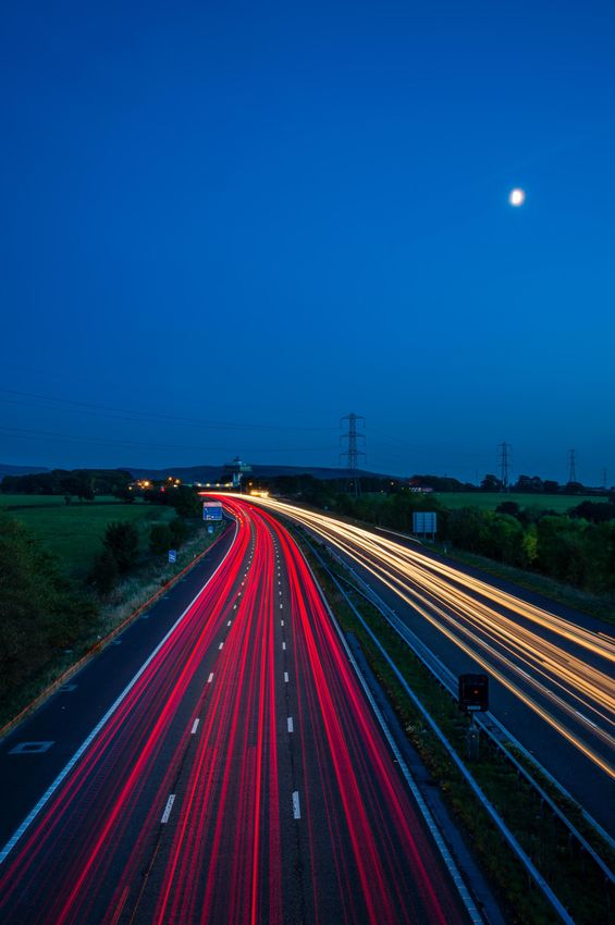
3.19 For High GDP, Low Fuel & Low GDP, High Fuel (scenario 2 and 3), we have applied
+/- 0.5 percentage points per annum to the growth rates in the reference scenario
from 2017 onwards. This is fed into the NTM, affecting the values of time. The GDP
inputs for High GDP, Low Fuel & Low GDP, High Fuel (scenario 2 and 3) are
displayed in Figure 10. The range for real GDP by 2050 is £3.2tn in Scenario 3 (Low
GDP, High Fuel) to £4.4tn in Scenario 2 (High GDP, Low Fuel) – a range of 38%.
22
https://assets.publishing.service.gov.uk/government/uploads/system/uploads/attachment_data/file/633077/national-travel-survey-
2016.pdf
32Costs of Driving
3.20 The cost of making a trip influences road traffic levels, informing an individual's
choice of whether to make a trip, how far they are willing to travel and what mode
they will use to make a trip. Within the NTM, costs primarily influence the trip
distribution and mode choice stages of the model. Costs can be broken down into
fuel and non-fuel costs. Non-fuel costs, which include oil, tyres, maintenance and
depreciation, are in line with WebTAG and are the same for all scenarios.
Post Tax Petrol Price
180
160
140
Fuel Cost per litre (pence) in 2015 prices
120
100
80
60
40
20
0
2000 2005 2010 2015 2020 2025 2030 2035 2040 2045 2050
Historic Scenario 1,4,5,6,7 S2 High GDP, Low Fuel S3 Low GDP, High Fuel
Figure 11: Post-Tax Petrol Price (Historic and Forecast)
3.21 There is uncertainty around future fuel prices (volatility in oil price), represented in the
Fossil Fuel Price Assumptions (FFPA) published by BEIS23. We have used the high
and low projections for road transport fuel prices in the FFPA to produce the post-tax
petrol price and diesel price. Post-tax petrol price can be seen in Figure 11 with
forecasts following a similar trend for diesel prices
3.22 Fuel costs combine the direct cost of fuel (per litre or per kilowatt hour (kWh) of
petrol, diesel or electricity) and the fuel efficiency of a vehicle. Fuel costs change
over time due to assumed improvements in fuel efficiency and forecast changes in
fuel prices.
3.23 High GDP, Low Fuel (scenario 2) takes the low fuel price projection. Low GDP, High
Fuel (scenario 3) takes the high fuel price projection. The range around the central
forecast in the FFPA for real petrol and diesel costs by 2050 will be approximately
29% and 32% respectively. The price of electricity does not vary in these scenarios.
23
https://www.gov.uk/government/publications/fossil-fuel-price-assumptions-2017
33Demand for Goods & Freight
3.24 The demand for goods is calculated using a forecast of the manufacturing index (see
Figure 12), a key input to the GBFM and the main driver of HGV traffic in the model.
In general the higher the demand for goods, the more goods need to be transported
and the higher HGV traffic on the roads. The manufacturing index is correlated with
GDP growth of the economy. Other key inputs include fuel prices and HGV fuel
efficiency forecasts.
3.25 The manufacturing index is produced by BEIS for energy demand and emissions
projections and forecasts manufacturing outputs based on lagged terms of the series,
GDP and terms of trade. Terms of trade are held flat at the last outturn and are an
ONS statistic. Therefore the main driver of the forecast series is GDP which varies in
these scenarios.
3.26 The forecasted manufacturing index has changed substantially since RTF15 and has
resulted in a lower forecast of HGV traffic growth. This has occurred for two reasons.
Firstly, BEIS, in conjunction with University College London have rebuilt their Industry
Growth Model (a regression model based entirely on historical correlation between
UK industrial growth, GDP and terms of trade). Secondly, RTF18 uses GDP
projections from the OBR which were updated in January 2018 following lower
productivity revisions.
Manufacturing Index
110
105
100
Index (2002=100)
95
90
85
0
80
2005 2010 2015 2020 2025 2030 2035 2040 2045 2050
Scenario 1,4,5,6,7 S2 High GDP, Low Fuel S3 Low GDP, High Fuel Historic
Figure 12 Manufacturing Index (Historic and Forecast)
34High Migration & Low Migration (Scenarios 4 & 5) – Context,
Assumptions & Inputs
3.27 These scenarios explore the uncertainty around population growth and distribution as
well as the relationship between car ownership and income for London.
Population Growth & Density
3.28 Population is another key driver of road traffic demand. As population continues to
increase there is a logical link to an increase in the aggregate level of road traffic.
Furthermore, the age and distribution of the population impacts on trip rates.
3.29 There has been a steady growth in population over the last 20 years which has
increased the overall demand for travel24. Population is fed into the model via NTEM.
The current version of NTEM uses ONS 2014 population projections.
3.30 Population growth is highly uncertain and difficult to predict. Figure 13 shows how
variable ONS population projections have been over the past 50 years and gives an
indication of the uncertainty surrounding population growth25.
Figure 13: Actual and projected UK population, 1951 to 2065, selected
projections by base year (ONS)
3.31 Although there has been a clear upward trend in the UK population and this is
expected to continue, the magnitude of this increase is uncertain and influenced by a
number of factors such as migration and number of births and deaths. Many of these
factors are difficult to predict themselves and can be altered dramatically by
unforeseen events. These often result in clear step changes in population growth.
24
https://assets.publishing.service.gov.uk/government/uploads/system/uploads/attachment_data/file/611304/annual-road-traffic-
estimates-2016.pdf
25
ONS National Population Projections Accuracy Report, 2016
353.32 Population projections become even more uncertain if broken down geographically
as other variables such as the number of houses available, availability of jobs and
migration between areas have a greater influence at this level. The spatial
distribution of population growth is a key factor in traffic growth particularly at regional
and local levels.
3.33 The 2015 National Travel Survey showed that those living in rural hamlets and
villages travel 90% further than those in urban conurbations26. In recent years, there
has been a trend towards more people living in urbanised areas where trips are often
shorter and public transport more likely to be used, but it is unclear as to whether this
trend will continue.
3.34 Modified ONS population projections are embedded within the NTEM dataset27.
While the spatial and demographic disaggregation of these is critical to producing
robust forecasts of traffic, understanding aggregate population changes is important
in understanding the overall trend in car use.
3.35 A key driver of road freight is consumer demand for goods28. Consumer demand is
related to the size of the population and so it is consistent to adjust freight traffic in-
line with any population changes.
3.36 Scenarios 4 and 5 use the 2014 ONS high/low migration population variants as a tool
for addressing both population growth and distribution uncertainty, allowing for a
practical way of manipulating the population between urban and rural areas given
migration tends to be focused in urban areas. This allows us to explore the possible
impacts of changes to trends regarding urbanisation.
3.37 High Migration (scenario 4) makes the following assumptions:
• An increase in net international migration, in line with the national high migration
variant produced by the ONS. This is distributed appropriately to the local
authorities with the highest migration to simulate urbanisation29.
• Decoupling of income to car ownership relationship in London
• HGV and LGV traffic increases in line with regional population assumptions, so
freight traffic increases more in urban areas and less in rural areas.
3.38 An increase in population in the model could lead to unrealistically high levels of car
ownership in London, where there is traditionally a higher proportion of public
transport usage. In order to mitigate this, we have assumed a decoupling of the
relationship between income and car ownership in London.
3.39 Decoupling refers to completely removing the link between income and a
household’s decision to purchase a car, meaning higher income people are no more
likely to own a car than people with lower incomes.
3.40 Historically, research has indicated that income levels positively influence road
demand but more recent studies are more mixed with some indicating the strength
and nature of this relationship may be changing30. Although higher income groups
still drive significantly more than those with lower incomes, the recent decline in car
26
Road Traffic Estimates 2016,
27
http://assets.dft.gov.uk.s3.amazonaws.com/tempro/version7/guidance/ntem-planning-data-guidance.pdf
28
Riet O, Jong G and Walker W (2007). ‘Drivers of Freight Demand and Their Policy Implication’.
29
ONS only produce high migration projections at the national level while they produce central migration projections at the local
authority level. To calculate the regional impact of high migration the national level increase has been distributed appropriately to the
local authorities which are projected to have the largest net migration under the ONS central migration projection.
30
Bastian, Anne, Maria Borjesson and Jonas Eliasson. 2016. "Explaining "peak car" with economic variables." Transportation Research
Part A: Policy and Practice 88pp 236-250.
36You can also read