Macroprudential Limits on Mortgage Products: The Australian Experience - Research Discussion Paper
←
→
Page content transcription
If your browser does not render page correctly, please read the page content below
Research Discussion Paper

                                  R D P 2021- 07

        Macroprudential Limits
         on Mortgage Products:
      The Australian Experience
Nicholas Garvin, Alex Kearney and Corrine Rosé
The Discussion Paper series is intended to make the results of the current economic research within the
Reserve Bank of Australia (RBA) available to other economists. Its aim is to present preliminary results of
research so as to encourage discussion and comment. Views expressed in this paper are those of the authors
and not necessarily those of the RBA. However, the RBA owns the copyright in this paper.
© Reserve Bank of Australia 2021
Apart from any use permitted under the Copyright Act 1968, and the permissions explictly granted below, all
other rights are reserved in all materials contained in this paper.
All materials contained in this paper, with the exception of any Excluded Material as defined on the RBA
website, are provided under a Creative Commons Attribution 4.0 International License. The materials covered
by this licence may be used, reproduced, published, communicated to the public and adapted provided that
there is attribution to the authors in a way that makes clear that the paper is the work of the authors and the
views in the paper are those of the authors and not the RBA.
For the full copyright and disclaimer provisions which apply to this paper, including those provisions which
relate to Excluded Material, see the RBA website.

Enquiries:
             Phone: +61 2 9551 9830
             Facsimile: +61 2 9551 8033
             Email: rbainfo@rba.gov.au
             Website: https://www.rba.gov.au

Figures in this publication were generated using Mathematica.

ISSN 1448-5109 (Online)
Macroprudential Limits on Mortgage Products:
                         The Australian Experience

                         Nicholas Garvin, Alex Kearney and Corrine Rosé

                                    Research Discussion Paper
                                            2021-07

                                             July 2021

                                  Financial Stability Department
                                    Reserve Bank of Australia

Thanks in particular to Bernadette Donovan, Aaron Mehrotra, Anthony Brassil, Carlos Cantu,
Sean Carmody, Jon Cheshire, Troy Gill, Jonathan Kearns, David Norman, David Rodgers and
Peter Tulip for feedback that improved this work in its various stages. The authors wrote this paper
while in the Financial Stability Department. The views expressed in this paper are those of the
authors and do not necessarily reflect the views of the Reserve Bank of Australia. The authors are
solely responsible for any errors. This paper builds on Corrine Rosé’s earlier work in her paper
Dobson (2020).

Authors: nick.j.garvin and alexander.g.kearney at domain gmail.com, roseco at domain rba.gov.au

                                 Media Office: rbainfo@rba.gov.au

                               https://doi.org/10.47688/rdp2021-07
Abstract

The Australian Prudential Regulation Authority implemented 2 credit limits between 2014 and 2018.
Unlike similar policies in other countries, these imposed limits on particular mortgage products – first
investor mortgages, then interest-only (IO) mortgages. With prudential bank-level panel data, we
empirically identify banks’ credit supply and interest rate responses and test for other effects of
these policies. The policies quickly reduced growth in the targeted type of credit while total mortgage
growth remained steady. Banks met the limits by raising interest rates on targeted mortgage
products and this lifted their income temporarily. The largest banks substituted into non-targeted
mortgage products while smaller banks did not. Practical implementation difficulties slowed effects
of the (first) investor policy, and led to some disproportionate bank responses, but had largely been
overcome by the time the (second) IO policy was implemented.

                           JEL Classification Numbers: E43, E5, G21, G28
               Keywords: macroprudential policy, banks, mortgages, mortgage rates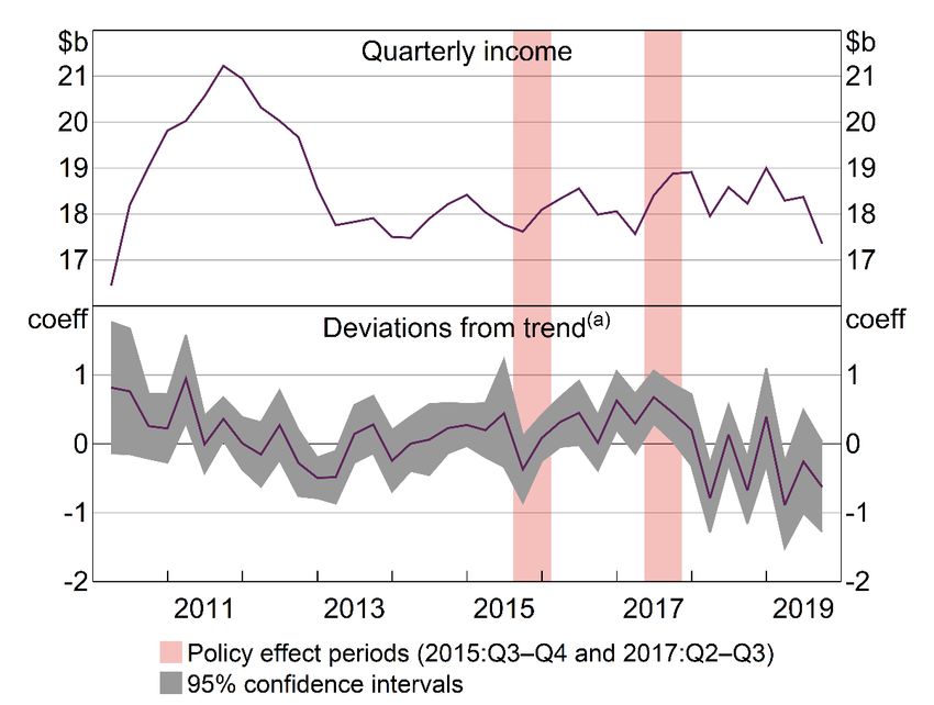
Table of Contents

1.   Introduction                                                               1

2.   The Credit Growth Limits                                                   3
     2.1     The investor mortgage limit                                        4
     2.2     The interest-only mortgage limit                                   5

3.   Data and Variables                                                         5
     3.1     Datasets and sample                                                5
     3.2     Regression variables                                               6

4.   Empirical Strategy                                                         9
     4.1     Average effect regressions                                         10
     4.2     Heterogeneous effect regressions                                   11

5.   Policy Effects of the Investor Limit                                       11
     5.1     Average effects on mortgage commitments                            12
     5.2     Average effects on advertised interest rates                       14
     5.3     Heterogeneous effects                                              17
     5.4     Assessing identification in the average effect analysis            19
             5.4.1    Placebo regressions                                       19
             5.4.2    The potential for coincidental credit trends              20

6.   Policy Effects of the Interest-only Limit                                  21
     6.1     Average effects on mortgage commitments                            22
     6.2     Average effects on advertised interest rates                       23
     6.3     Heterogeneous IO-policy effects                                    24
     6.4     Placebo regressions                                                26

7.   Other Mortgage Market Outcomes                                             26
     7.1     Policy effects by loan-to-valuation ratio                          27
     7.2     Policy effects on aggregate variables                              28
             7.2.1    Effects on aggregate housing and business credit growth   29
             7.2.2    Effects on market concentration                           30
             7.2.3    Effects on banks’ pricing power                           32
     7.3     Loan-type switching                                                33
     7.4     The cyclicality of mortgage products                               34

8.   Conclusions                                                                35

References                                                                      37

Copyright and Disclaimer Notice                                                 40
1. Introduction
Twice between 2014 and 2018, the Australian Prudential Regulation Authority (APRA) temporarily
restricted banks’ lending in mortgage types considered systemically risky. The first policy, announced
late 2014, required banks to limit their lending to housing investors, or in other words, ‘buy-to-let’
borrowers that will rent out the housing. The second policy, announced early 2017, imposed limits
on interest-only (IO) mortgages, in which the loan principal stays constant and only interest is repaid.
APRA (2019b) describes the policies as ‘tactical, temporary constraints’, because they were designed
to act fast and target the specific sources of systemic risk. Credit was expanding rapidly in residential
mortgage products considered procyclical, while housing prices and household debt were high and
rising (Debelle 2018; APRA 2019b). The limits were later removed, replaced by longer-term
solutions.1
Macroprudential credit growth limits are backed by a deep literature tying credit growth to financial
crises. Research shows that excessive credit growth is the most consistent antecedent of financial
crises (e.g. Borio and Lowe 2002; Reinhart and Rogoff 2011; Schularick and Taylor 2012).
Speculative mortgage debt and housing price cyclicality were fundamental ingredients in the 2008
financial crisis (Adelino, Schoar and Severino 2016; Foote, Loewenstein and Willen 2021), and
contributed to crises further back (Dell’Ariccia et al 2012; Richter, Schularick and Wachtel 2021).
The evidence has led to policy action. A variety of macroprudential tools have been implemented to
curb excessive or risky credit (e.g. Cerutti, Claessens and Laeven 2017), including many specifically
targeting mortgage lending (e.g. Kuttner and Shim 2016).
To our knowledge, none of these policies have targeted overall growth in particular mortgage
products, aside from APRA’s.2 APRA’s first policy required each bank to limit its year-ended growth
in investor housing credit to 10 per cent. The second policy required each bank to limit its quarterly
new IO mortgage lending to 30 per cent of total new housing lending. Most policies in other countries
have set quantitative requirements only on loans above specific loan-to-valuation ratios (LVRs) or
loan-to-income ratios (LTIs). APRA did present guidance that banks should manage new lending at
high LVRs and LTIs, but quantitative limits were only set for the specific mortgage products. This
was for a few reasons: high LVR lending was already in decline, limits on high LVR loans can
disproportionately affect first home buyers, and the main risks appeared concentrated in speculative
and IO borrowing (Ellis and Littrell 2017; APRA 2019b).
Our paper presents a bank-level panel data study of banks’ reactions to the policies. We present
causal statistical evidence, with falsification tests, that the policies reduced growth in the policy-
targeted mortgage products. Banks cut lending growth in targeted mortgages by around 20 to
40 percentage points within a year of the policy announcements. While conclusions about systemic
stability are outside this paper’s scope, the findings are consistent with the policies achieving their
objectives. We also present 3 conclusions, which build on existing qualitative analysis of the policies
by the Australian Competition and Consumer Commission (ACCC), APRA and the Australian
Government Productivity Commission (PC):
1 These include proposals to differentiate capital risk weightings by mortgage types (APRA 2020) and APRA’s July 2019
amendments to official guidance for banks on sound residential mortgage lending (APRA 2019a).
2 The closest to APRA’s appears to be Singapore’s 2009 ban on IO mortgages, described in Upper (2017).2
1. Banks cut back targeted mortgage types by raising interest rates on those
mortgages. This has been noted by, for example, ACCC (2018a, 2018b). We contribute by
presenting causal statistical evidence, which estimates policy-induced rises in advertised rates
of around 10 to 30 basis points, and by tying together banks’ quantity and price responses.
These rate rises partly reflected a desired repricing of risk, although ACCC (2018a, 2018b) also
argue that the policies presented a focal point for coordinated anti-competitive price changes.
We find that banks’ mortgage interest income rose after the IO policy, in line with the ACCC’s
conclusion, but that the effect was short-lived.
2. Banks’ policy reactions depended on their size. Large banks – that is, the 4 Australian
major banks – substituted into non-targeted mortgage types, and sustained their overall
mortgage growth. The 20 or so other (mid-sized) banks in our sample did not substitute and
their overall mortgage growth declined. These bank-level patterns are statistically significant
but, in aggregate, coincide with only a small temporary pick-up in large banks’ mortgage market
share relative to the other sample banks. To our knowledge we are the first to show that banks’
credit allocation reactions to macroprudential policies depend on their size.
3. Implementation difficulties significantly influenced how the policies played out.
Banks reacted to the investor policy with a 2-quarter delay, and their reaction sizes were
misaligned with the policy impositions. These results support conclusions in previous regulatory
reports that banks’ systems initially lacked the capacity to control growth in the targeted
mortgage types, and, for mid-sized banks, this imperfect control was compounded by heavy
customer flows from the large banks’ policy reactions. Contacts also tell us that some banks
were uncertain about the precise definition and time frame for the investor limit, which
contributed to the delayed reactions. Practical difficulties were less prevalent for the IO policy,
after banks had improved their systems, and with the policy worded more precisely.
Our work presents several other results. Analysis of aggregate credit indicates that the policies had
little effect on overall housing credit growth – with large banks substituting across housing credit
types – and, if anything, a positive effect on business credit. Analysis of granular mortgage
categories reveals that the accompanying guidance on high LVR lending, mentioned above,
interacted with the quantitative limits: the decline in targeted housing credit was concentrated in
high LVR loans, and substitution into non-targeted housing credit was concentrated in low LVR loans.
We also argue that the substitutability between targeted and non-targeted mortgages differed across
the 2 policies due to the types of products targeted. While a bank can steer any given customer
towards either an IO or a principal and interest (P&I) loan, by offering attractive interest rates
(e.g. Guiso et al forthcoming), customers typically cannot switch their status from investor to
occupier. Therefore, to substitute from investor to occupier credit, banks need to find other
customers, which Acharya et al (2020) call the ‘bank portfolio choice’ channel. This likely made
substitution easier under the IO policy relative to the investor policy. More generally, across the full
sample we find that IO and investor lending move with housing prices, while occupier P&I lending
does not. This is consistent with speculative demand being driven by recently observed price
behaviour.
This paper contributes to the growing literature studying the variety of macroprudential credit growth
policies implemented around the world. In line with the other policies implemented, most papers
focus on the impact of LTI and LVR limits. Results typically show a reduction in the targeted3 mortgages, particularly by banks exceeding specified limits. Some find that banks under the limits lift mortgage originations, in targeted mortgages (in the United Kingdom, Peydró et al (2020)), or in non-targeted mortgages (in Ireland, Acharya et al (2020)). We find that substitution into non- targeted mortgages is mostly by banks above the limits, which in our sample tend to be the largest banks, with potentially more capability to shift their portfolios. Many studies also find a significant negative effect on housing prices, including in the United Kingdom (Peydró et al 2020), in New Zealand (Armstrong, Skilling and Fao 2019) and in cross-country studies (Kuttner and Shim 2016; Alam et al 2019; Araujo et al 2020). We do not analyse housing price effects, but note that RBA (2018) finds that the investor policy caused housing price growth to slow more in investor- concentrated regions than in occupier-concentrated regions. More broadly, ours and these other papers on credit growth limits contribute to the wider literature on macroprudential policy effects (e.g. Aiyar, Calomiris and Wieladek 2014; Cerutti et al 2017; Jiménez et al 2017). Banks’ use of interest rates to target credit growth has been less studied. Basten (2020) shows that, following the introduction of the countercyclical capital buffer (CCyB) in Switzerland, capital- constrained banks raise their mortgage rates more than others. DeFusco, Johnson and Mondragon (2020) show that US lenders charge a premium of 10 to 15 basis points to originate loans above a regulatory debt-to-income ratio threshold (under the Dodd Frank Act), above which mortgages require extra ‘ability to repay’ documentation. We find interest rate policy effects of a similar magnitude. They also find that banks additionally contained quantities through credit rationing, which led to irregular demand elasticities, and we also find that banks limited credit supply through means other than rate rises. The rest of this paper is laid out as follows. We first describe the investor and IO policies (Section 2). As background for the analytical results, the next sections explain the dataset and the variables of interest (Section 3) and the econometric models we use (Section 4). Then we report results for policy effects on banks’ credit growth and interest rates, first for the investor policy (Section 5), and then for the IO policy (Section 6). Section 7 presents findings for other outcomes of interest: banks’ LVR distributions (7.1); aggregate credit trends (7.2.1); banks’ housing credit market shares (7.2.2); banks’ mortgage pricing power (7.2.3); borrowers’ reclassifications of mortgage types (7.3); and, more generally, the cyclicality of mortgage behaviour throughout the sample (7.4). Section 8 concludes. 2. The Credit Growth Limits APRA’s 2 macroprudential policies were announced in late 2014 and early 2017, respectively. The policy designs had 4 goals: efficient and well-targeted on the identified risks; competitively neutral across the industry, but with flexibility for smaller banks; able to be implemented quickly and simply; and able to be dialled up or down as required (APRA 2019b). The 2 quantitative limits were the most significant components of a package of measures that more broadly increased the intensity of housing lending oversight. The overarching objectives of this package were to strengthen the resilience of individual ADIs, and to promote the stability of the financial system overall.3 The policies were supported by the Council of Financial Regulators, which comprises APRA, the Australian Securities and Investments Commission, the Reserve Bank of Australia (RBA), and the Australian Treasury. The risk environment that led to the policies is described in most detail by 3 ADIs stands for authorised deposit-taking institutions. In most instances, this paper loosely refers to ADIs as banks.
4

RBA (2018). The main concern was that the targeted mortgage types were contributing to a housing
market upswing that raised the risk of a subsequent economic downturn. Alongside rapidly rising
investor housing credit, housing prices were rising and household debt was growing at its fastest
pace in around a decade. This presented the risk that if income or housing prices subsequently fell,
highly indebted households might react with a sharp reduction in consumption.

The rest of this section provides more details on the 2 quantitative limits.

2.1      The investor mortgage limit

APRA announced the investor limit on 9 December 2014 through a public letter to ADIs. Letters to
ADIs do not constitute binding prudential requirements, but can present information about how
APRA will exercise discretionary regulatory powers. The letter states that:

      ... annual investor [housing] credit growth materially above a benchmark of 10 per cent will be an
      important risk indicator that supervisors will take into account when reviewing ADIs’ residential
      mortgage risk profile and considering supervisory actions. (APRA 2014)

In the following months, the expectations that banks comply with the limit were ramped up.
APRA (2019b, p 13) writes that:

      … over the first half of 2015, APRA supervisors took coordinated action to reinforce the objectives of the
      benchmark with all ADIs and obtain action plans for meeting it … In a number of cases, supervisors agreed
      on an appropriate timeline for meeting the expectations with individual ADIs …

By August, the 4 largest banks had each indicated to the RBA that they were then treating the
benchmark as a hard limit.4 The policy remained less strict for small banks with mortgage portfolios
of less than $1 billion, which were given a longer horizon to comply.5

The letter to banks also stated that APRA would monitor other types of banks’ lending. The other
types included high LVR and high LTI mortgages, IO mortgages, mortgages with very long terms,
and mortgages that did not perform well on borrower affordability tests. However, no quantitative
requirements were stated for those mortgage types, then or later. We focus on the effects of the
quantitative limits, but also analyse policy effects by LVRs in Section 7.1.

APRA removed the investor limit in April 2018, conditional on banks’ boards providing assurance of
ongoing safe lending practices. The limit was removed due to the actions banks had taken to improve
the quality of their lending (APRA 2019b). It was replaced with longer-term tools for distinguishing
between mortgage products in their systemic risk contributions. In February 2018, APRA released
proposed changes to ADIs’ capital framework that would impose higher risk weights for investor
mortgages than occupier mortgages, and reaffirmed its proposal in December 2020. Additionally, in
July 2019, APRA released a revised Prudential Practice Guide that outlined APRA’s interpretation of
prudent practices in residential mortgage lending (APRA 2019a), to supplement APRA’s legally
enforceable Prudential Standards.

4   This was communicated in the RBA’s regular liaison with banks.
5   These banks are below the size threshold for inclusion in our sample (Section 3.1).
5
2.2 The interest-only mortgage limit
APRA announced the IO limit on 31 March 2017 in another letter to ADIs. The letter asked banks to
limit new IO lending to no more than 30 per cent of total new mortgage lending. From the start, the
expectations were stricter than for the investor policy. The letter states ‘APRA supervisors … will
likely impose additional requirements on an ADI if the proportion of new lending on interest-only
terms exceeds 30 per cent of total new mortgage lending, over the course of each quarterly period’,
and ‘APRA expects all ADIs to immediately take steps’ (APRA 2017). IO mortgages were a concern
in part because the lack of amortisation keeps the borrower’s leverage higher for longer, and in part
because IO mortgages automatically convert to P&I loans, usually after 5 to 10 years, which can, if
the mortgage is not refinanced to another IO loan, bump up the repayments and can cause distress
for the borrower (Kent 2018).
APRA also noted it would monitor other metrics of risk in banks’ new mortgage lending, in a similar
manner to the guidance accompanying the investor limit. Again, there were no quantitative
requirements on those metrics. In December 2018, APRA removed the limit, stating that the policy
had served its purpose.
3. Data and Variables
This section details the data, sample and variables used for the empirical analysis. Section 3.1
describes the data sources and the sample choices. Section 3.2 defines the regression variables and
provides summary statistics.
3.1 Datasets and sample
The two main data sources comprise banks’ confidential data reporting to APRA, and banks’
advertised mortgage rates from the subscription-based Canstar database. We supplement these with
housing price data from the subscription-based CoreLogic database and publicly available national
accounts data from the Australian Bureau of Statistics (ABS).
The sample is quarterly, from 2008:Q1 to 2019:Q3, and covers banks with at least $1 billion in total
loan assets. The regression samples each exclude banks that were not in the sample one year prior
to the policy announcement, leaving around 28 banks in most cases. Sample banks are classified as
either large or mid-sized. The large banks comprise the 4 major banks – ANZ, CBA, NAB and Westpac
– which are each similar sized, and together hold around 80 per cent of total mortgage credit in
Australia. The remaining banks are much smaller and classified as mid-sized. There were 3 mergers
between sample banks during the sample period, so for the quarters prior to the merger, we combine
the 2 pre-merged banks into 1 consolidated entity.
To analyse new housing lending, we use data on mortgage commitments. A mortgage commitment
takes place after the borrower receives an accepted and signed offer of credit from the lender,
typically after the borrower has signed the contract for purchase of the property.6 Commitments are
6 Technically, our data are on approvals rather than commitments, but the 2 concepts are very similar in definition and
empirically, and ‘commitments’ is now the more commonly used term. An approval occurs once the borrower receives
the signed and accepted offer of credit from the lender; a commitment occurs once the borrower signs that offer and
hands it back to the lender.6
categorised by either the borrower type (occupier or investor), or by the repayment structure (P&I
or IO), or by both. Commitments are a better measure of mortgage origination than changes in
credit outstanding, for 2 reasons. First, following the policy announcement in December 2014, banks
raised interest rates on investor mortgages (Section 5.2), and many customers updated their bank
about their classification as an investor or occupier. This heavily affected credit quantities
outstanding, despite not generating mortgage originations, but only rarely would have affected
commitments. These reclassifications are discussed further in Section 7.3. Second, credit
outstanding can move for reasons unrelated to new lending, such as refinancing, early repayments,
or drawing down on excess balances. Nonetheless, commitments do not perfectly map to new
mortgage lending (i.e. originations), which was the target of the limits. Commitments typically lead
originations by a few weeks, and in some cases result in no origination.
The Canstar data on advertised mortgage rates cover various mortgage subtypes and require some
discretionary alignment with the 4 categories of approvals (occupier P&I, occupier IO, investor P&I,
investor IO).7 It is important to note that the advertised rates do not cleanly represent rates charged.
Borrowers often receive a discount on the advertised rate, which is more common among large
banks than mid-sized banks. Our analysis of advertised rates could therefore miss policy effects on
discounts, which did occur to some extent (e.g. ACCC 2018b). However, when analysing targeted
mortgages, this would more likely understate than overstate the policy effect estimates. That is,
given that banks were using rates to reduce demand for targeted mortgages (Sections 5.2 and 6.2),
discounts were more likely to be lowered rather than raised, in which case the rises in advertised
rates would understate the rises in offered rates. For non-targeted mortgages, the opposite holds
true, so it is possible that those estimates of policy effects on interest rates are overstated,
particularly for large banks.
3.2 Regression variables
The 2 main dependent variables are commitments growth ( CommitGrthbm,t ) and mortgage
rates ( IntRatebm,t ). CommitGrthbm,t measures the percentage change in the total dollar value of
mortgage commitments from quarter t 1 to quarter t , for mortgage type
m investor , occupier , IO, P & I , Total and by bank b . It is expressed as a decimal, so, for
example, 10 per cent growth is 0.1. All infinite values are excluded (i.e. when a bank grows
commitments from zero) and remaining outliers above 300 per cent are truncated to 3.
The dependent variable IntRatebm,t measures bank b ’s advertised mortgage rate at the end of
quarter t , minus the cash rate, in percentage points. It is first differenced in most regressions. When
analysing the investor policy, ‘investor rates’ are from investor P&I mortgages, and ‘occupier rates’
are from occupier P&I mortgages. When analysing the IO policy, ‘IO rates’ are from investor IO
mortgages and ‘P&I rates’ are from investor P&I mortgages. This approach varies the mortgage-
7 Details of the alignment are as follows. Most banks offer multiple mortgage packages within some categories, such as
one ‘basic’ occupier P&I package and another high LVR occupier P&I package. In most cases, there is a single ‘standard
variable rate’ package for each of the occupier P&I, investor P&I and investor IO categories, and we use these
wherever possible. This helps for consistent alignment across banks. Where this alignment is not possible, we align
mortgage packages with the commitments categories based on what alignment gives the least series jumps from
discontinuance of particular packages. Prior to the policies, many banks did not operationally distinguish the targeted
loan type from the non-targeted type, including in the interest rate charged. In these cases, interest rates are reported
for only one category, which we apply to both mortgage types in our sample.7
type dimension affected by the policy while holding the other dimension constant. It also avoids
relying on rates for occupier IO mortgages, which are less common than other mortgage types.
The 2 key explanatory variables are a bank-invariant indicator variable for the quarter a policy is
announced ( policy t ) and a measure of how far bank b is from the policy limit ( Treatmentb ,t ).
policy t is one in the quarter t the policy is announced, and zero in other quarters. Most
regressions use its first to fourth lags, which capture policy effects in the 4 quarters after the
announcement. Treatmentb ,t takes 2 alternative forms: linear and binary. For the investor policy,
the linear measure is the bank’s year-ended growth in the total value of investor mortgages
outstanding, minus 10 per cent, measured in percentage points.8 For the IO policy, the linear
measure is the proportion of the bank’s quarterly housing commitments that are IO commitments,
minus 30 per cent, measured in percentage points. As noted in Section 3.1, the policy referred to
the proportion of new mortgage lending, but we do not have data on originations, so we use
commitments as a close proxy. The binary form of Treatmentb ,t is an indicator variable for whether
bank b is above the limit in quarter t , or in other words, for whether the linear form of Treatmentb ,t
is positive.
The regressions also include sets of macroeconomic and bank-level control variables. The (bank
invariant) macroeconomic controls include quarterly growth in national GDP (from the ABS),
quarterly growth in national housing prices (from CoreLogic), and the first difference in the quarter-
end ‘cash rate’, which is Australia’s key monetary policy rate (from the RBA).9 These are all expressed
in percentages. The macroeconomic controls also include a set of seasonal indicator variables that
control for the 4 quarters each year – for example, a ‘Q2’ indicator, which is 1 in Q2 each year and
0 in other quarters – because commitments tend to be highly seasonal (evident in Figure 1 below).
In the regression formulas, the vector of macroeconomic controls is represented by MacroControlst .
The bank-level controls are the tier 1 capital ratio and the ratio of deposit liabilities over total
liabilities, both expressed in percentage points, sourced from the confidential APRA data. These are
represented in the regression formulas by BankControlsb,t .
The regression variables are summarised in Table 1. Most of the regression samples separate large
from mid-sized banks. The size difference between large and mid-sized banks is clear from the
commitments values. Large banks’ mean value of quarterly total commitments is $14.8 billion, with
a $4.5 billion standard deviation, while mid-sized banks’ mean is $0.9 billion and standard deviation
is also $0.9 billion. Commitments growth rates are similar for large and mid-sized banks, but vary
more across mortgage types for mid-sized banks. Large banks tend to advertise higher spreads than
mid-sized banks, but this likely reflects that large banks more commonly offer discounts off the
advertised rate. (The regressions mostly analyse changes in spreads, so any time-invariant influence
of discounting would be removed.) Mid-sized banks rely on deposit funding more so than large
banks.
8 One of the large banks reported an infeasible jump in investor credit outstanding in 2014:Q4 ($24 billion or 45 per
cent), accompanied by a very large decline in occupier credit outstanding ($13 billion). This jump appears to be a
reclassification of pre-existing credit from occupier to investor, so we adjust the data by adding $13 billion to that
bank’s investor credit in all quarters before 2014:Q4.
9 We use non-farm, chain volume, seasonally adjusted GDP.8
Table 1: Regression Variable Summary Statistics
Large banks Mid-sized Full sample
banks
Mean SD Mean SD Min 25% Median 75% Max Number
Mortgage commitments quarterly value ($b)
Investor 5.2 2.2 0.3 0.3 0.0 0.1 0.2 0.8 11.3 946
Occupier 9.6 2.8 0.6 0.6 0.0 0.2 0.6 1.8 17.1 946
Interest only (IO) 5.0 2.7 0.2 0.3 0.0 0.0 0.2 0.8 12.7 946
Principal and interest 9.8 3.8 0.7 0.7 0.0 0.2 0.6 1.9 20.0 946
(P&I)
Total 14.8 4.5 0.9 0.9 0.0 0.3 0.8 2.6 26.3 946
Mortgage commitments quarterly growth (%)
Investor 8.4 46.8 11.0 49.5 –100.0 –13.5 2.6 22.5 300.0 918
Occupier 8.1 45.6 6.7 34.9 –94.6 –10.7 2.2 16.4 300.0 919
IO 7.5 48.6 10.9 55.7 –100.0 –16.8 0.7 24.2 300.0 916
P&I 8.6 45.5 7.4 37.1 –94.8 –10.5 2.2 17.0 300.0 919
Total 8.0 45.6 6.5 34.4 –95.5 –10.4 1.6 16.1 300.0 919
Change in mortgage rate spread to cash rate (to quarter-end, bps)
Investor P&I 4.4 10.2 2.1 20.5 –238.0 0.0 0.0 5.5 80.0 1,133
Occupier P&I 3.0 11.9 1.3 17.6 –162.0 0.0 0.0 2.0 75.0 1,183
P&I investor–occupier 1.5 12.9 0.7 14.0 –80.0 0.0 0.0 0.0 89.0 1,130
spread
Investor IO 5.3 12.5 2.5 22.5 –246.0 0.0 0.0 9.0 80.0 944
Investor IO–P&I 0.9 8.6 0.1 11.9 –136.0 0.0 0.0 0.0 157.0 929
spread
Bank-level control variables (%)
Tier 1 capital ratio 11.1 1.5 13.7 4.6 6.5 10.4 12.2 15.1 32.5 984
Deposit over liabilities 47.8 7.3 71.0 21.2 11.8 46.9 67.8 86.4 99.0 984
ratio
Sources: APRA; Authors’ calculations; Canstar; RBA
Figure 1 displays the aggregate behaviour of some key variables. Most commitments are for occupier
P&I mortgages, with the remaining commitments roughly equally split across the other 3 mortgage
types, until around 2013 when investor IO commitments pick up (top panel). Commitments have
clear seasonality in a 4-quarter cycle. Average mortgage rates across banks are initially very close
for different mortgage types, until after the first policy announcement in late 2014 (middle panel).
Comparing the middle and bottom panels makes clear that mortgage rates move fairly closely with
the cash rate. The most noteworthy behaviour in the macroeconomic variables is in 2015, when the
investor policy was being implemented (bottom panel). In the first half of 2015, the cash rate is cut
twice – by 25 basis points in both February and May – but it remained constant for the rest of 2015,
and throughout 2017 and 2018. Also in the second half of 2015, housing price growth declined from
around 5 per cent per quarter to around zero. This is discussed briefly in Section 5.4.2.9
Figure 1: Mortgage Aggregates and Macro Controls
Quarter-end
$b Total mortgage commitments $b
Quarterly flow
90 90
60 60
30 30
% Average advertised mortgage rates(a) %
7 7
6 6
5 5
Occupier P&I Occupier IO Investor P&I Investor IO
% Macroeconomic controls %
Cash rate
4 4
0 0
GDP growth
Housing price growth
-4 -4
2009 2011 2013 2015 2017 2019
Note: (a) Mortgage rates as used in regressions, after cleaning and alignment; unweighted average across banks
Sources: ABS; APRA; Canstar; CoreLogic; RBA
4. Empirical Strategy
We identify policy effects with 2 types of panel data regressions. The first detects the average policy
effect across all banks in the sample that is used. We supplement these estimates with falsification
(i.e. placebo) tests that gauge the likelihood of falsely identifying policy effects. The second type
detects policy effects that systematically differ across banks. The second type has a more robust
identification strategy, so it provides a more definitive test of whether the policies caused a change
in banks’ behaviour. However, aggregate policy effects are less clear with this specification, hence
the use of 2 separate strategies. Note that none of the specifications give more weight to banks with
larger portfolios, so the outcomes should not be interpreted as aggregated effects on the banking
system. (But that interpretation would be close for samples containing only the 4 large banks.) To
understand aggregated effects we report aggregate time series throughout various parts of the
paper.10
4.1 Average effect regressions
The average effect regressions estimate the policy effects using (bank invariant) indicator variables
for the 4 quarters after the policy announcement ( policy t 1, ,t 4 ). Control variables remove other
influences, leaving the indicator variables to capture any ‘abnormal behaviour’ in the policy period
that is common across all banks in the sample. The controls include lagged dependent variables,
other bank-level control variables, and system-level macroeconomic control variables.
The average effect regression equation is
4 K
CommitGrthbm,t j policy t j k CommitGrthbm,t k
j 1 k 1 (1)
BankControlsb,t MacroControlst b,t
In Equation (1), the lagged dependent variables are instrumented using the Arellano–Bond
procedure. This involves first differencing all variables (as per Equation (1)). Bank fixed effects are
therefore not included. The macro controls are GDP growth, housing price growth and the set of
seasonal controls.10 The bank controls are the capital ratio and the deposit funding ratio, both lagged
once to address reverse causality.
The average effect specification for mortgage interest rates is
4
IntRatebm,t b 1 j policy t j BankControlsb,t MacroControlst b,t (2)
j 1
where b is a set of bank-level fixed effects. The bank and macro controls are the same as in
Equation (1), except the first 2 lags of the quarter-end change in the cash rate are added as macro
controls, given that the cash rate is a very strong determinant of mortgage rates. Lagged dependent
variables are included in Equation (1) but not in Equation (2), because mortgage rate changes are
much less persistent than commitments growth.
The average effect regressions are repeated for mortgage types m not targeted by the policies.
These non-targeted mortgages serve as a quasi control group. For example, if a decline in credit
that is detected by policy is instead spuriously driven by macroeconomic influences, this should
be revealed by a negative policy effect in the non-targeted loan types. It is not appropriate to use
non-targeted mortgages as an explicit control group in a differences-in-differences specification. This
would lead to overstated policy effect estimates if banks substituted from targeted to non-targeted
mortgages. However, we are still interested in the effects of the policy on non-targeted mortgages.
So we examine them in separate estimations, but without including them as explicit controls in the
same equation.
10 Including the cash rate as a control has little effect on the policy effect estimates. We do not include it because its
true effect on commitments is likely to be slow and cumulative, and its coefficients indicate that it is picking up effects
not caused by the cash rate.11
The main threat to identification is the possibility of system-wide influences that coincidentally affect
(only) targeted mortgages when the policies are implemented, and that are not captured by the
control variables. We address this in 2 ways. First, we run placebo regressions akin to the falsification
tests suggested by Roberts and Whited (2013). In the placebo regressions, the 4 policy variables
are swapped for a ‘placebo’ indicator variable that instead indicates a single non-policy quarter, to
assess whether a false positive effect shows up in that quarter. This is repeated for all non-policy
quarters from 2010 onward. If few of these placebo indicators are significant, the likelihood of
coincidental factors causing a falsely detected policy effect is low. Due to the multiple testing problem
(e.g. Bender and Lange 2001), these placebo tests warrant conservative significance thresholds,
which we acknowledge informally. We also address the coincidental-influences identification threat
with a qualitative analysis of economic trends that could have potentially generated false policy
effects.
The average effect regressions are each run on multiple samples. One sample comprises only the
4 large banks, another sample comprises only mid-sized banks and a third sample comprises all
banks.
4.2 Heterogeneous effect regressions
The heterogeneous effect regressions identify policy effects that differ across banks, in line with how
close those banks are to satisfying the policy limits. Intuitively, banks above the limit should be more
intensely ‘treated’ by the policy than banks below. Focusing on these differences in reactions across
banks allows including fixed effects for each quarter, which in the average effect regressions would
be collinear with policy . Quarter fixed effects remove all system-wide influences on the
dependent variables, and give a stronger case for identification of the policy effects.
The heterogeneous policy effects regression equation is
4
Ybm,t b t 1 j policy t j Treatmentb,t 2 BankControlsb,t b,t (3)
j 1
Y is either CommitGrth or IntRate , and Treatment is a measure of how far bank b is above
the limit. Treatment is lagged twice to remove reverse causality from mechanical dependence on
commitments growth.11 That is, distance from the limit in a given period likely depends on
commitments in that period, and therefore on commitments growth in the next period (because
growth rates depend on the level in the last period). Bank and quarter fixed effects are represented
by b and t . The bank controls are the capital ratio and deposit funding ratio.
5. Policy Effects of the Investor Limit
The investor mortgage limit, announced in December 2014, limited banks’ growth in investor housing
credit to 10 per cent per annum. Other regulatory reports document that the limit took time to
implement (e.g. APRA 2019b), as APRA worked with banks to clarify their obligations (as noted in
Section 2.1) and banks worked on improving their systems for implementing the policy. Contacts tell
11 Treatment is chosen as a rolling measure, rather than fixed at the time of the policy announcement. This is because
if a bank moves to below the benchmark soon after the policy announcement (for example), then it is unlikely to still
behave as though it is above the benchmark.12
us that banks also initially faced some confusion over the definition of the limit, for example, about
how to treat pre-existing investor credit that was being reclassified as occupier credit (analysed in
Section 7.3), or whether the limit applied to raw or seasonally adjusted credit growth figures. A delay
between the policy announcement and its effect is indeed evident in the aggregate data (Figure 2).
Aggregate investor commitments growth remains flat in 2015:Q1 and Q2, then declines sharply in
2015:Q3 and Q4 alongside a pick-up in occupier commitments growth (top panel). The number of
banks above the limit picks up in 2015:Q1 and Q2, but, from 2015:Q3 onward, steadily declines
towards zero (bottom panel).
Figure 2: Investor Mortgages
% Aggregate quarterly commitments growth %
40 40
20 20
0 0
Occupier mortgages
-20 -20
Investor mortgages
no Banks exceeding 10% year-ended investor credit growth(a) no
12 12
8 8
4 4
Policy announcement
0 0
2012 2013 2014 2015 2016 2017
Notes: The number of banks in the sample varies slightly across periods but is constant from 2014:Q3 to 2017:Q4
(a) May not perfectly align with APRA’s assessment of banks meeting the limit
Sources: APRA; Authors’ calculations
5.1 Average effects on mortgage commitments
In the full sample of banks, the policy effect on targeted mortgages is negative, large and statistically
significant in 2015:Q3 and Q4 (Table 2, column (a)). The coefficients imply a decline in investor
commitments growth of 51 percentage points across these 2 quarters, for the average bank.12 There
are no significant policy effects in the first 2 quarters, in line with the aggregate data (Figure 2),
implying a 2-quarter delay from the policy announcement on average. Non-targeted mortgages
increase by a statistically insignificant and small amount (column (b)), which implies that the
estimated investor policy effects in column (a) are not mistakenly picking up trends in aggregate
housing credit. Total mortgage commitments for the average bank are not significantly affected
(column (c)). Therefore, the large reduction in investor commitments growth is mostly offset by the
small pick-up in occupier commitments growth.
12 The calculation for the cumulative effect on growth is 1 – (1 – 0.235) × (1 – 0.337).13
Table 2 Average Effects of Investor Limit on Mortgage Commitments
Regression coefficients, standard errors in parentheses
(a) (b) (c) (d) (e) (f) (g) (h) (i)
Sample All Large Mid-sized
banks:
Mortgage Investor Occupier Total Investor Occupier Total Investor Occupier Total
type:
Q1 15 –0.058 0.024 0.015 –0.025** –0.008 –0.008 –0.070 0.029 0.019
(0.052) (0.039) (0.039) (0.011) (0.011) (0.007) (0.062) (0.047) (0.047)
Q2 15 –0.051 0.005 –0.013 –0.059 0.020 0.003 –0.031 0.002 –0.010
(0.070) (0.056) (0.056) (0.072) (0.071) (0.072) (0.085) (0.067) (0.066)
Q3 15 –0.235*** 0.029 –0.061 –0.236*** 0.144* –0.025 –0.241*** –0.005 –0.072
(0.072) (0.054) (0.049) (0.032) (0.086) (0.051) (0.089) (0.060) (0.057)
Q4 15 –0.337*** 0.024 –0.080 –0.025 0.096** 0.055 –0.423*** 0.002 –0.116**
(0.094) (0.057) (0.049) (0.051) (0.044) (0.036) (0.108) (0.069) (0.057)
Lagged DVs 2 2 2 2 2 2 2 2 2
Controls yes yes yes yes yes yes yes yes yes
Sample size 686 686 686 168 168 168 518 518 518
Notes: Coefficients from panel regressions, across banks and quarters, of commitments growth on 4 lags of the bank-invariant policy
indicator variable. The full equation is in first differences, using Arellano–Bond, with 2 lagged dependent variables (DVs) to
eliminate second order autocorrelation. The control variables are GDP growth, housing price growth, lagged tier 1 capital
ratios, lagged deposit funding ratios and a set of seasonal dummy variables. ***, ** and * denote statistical significance at
the 1, 5 and 10 per cent levels, respectively.
The full sample estimates mask sizeable differences in reactions between large and mid-sized banks.
Most notably, large banks substitute into non-targeted mortgages while mid-sized banks do not.
Large banks’ substitution into occupier commitments (column (e)) offsets their investor
commitments growth decline, leaving no significant change in total mortgage commitments (column
(f)). Mid-sized banks do not increase occupier commitments growth (column (h)), leaving a
statistically significant net decline in total commitments growth of 12 percentage points (column (i)).
The reason for this difference in substitution behaviour is not entirely clear, but it is plausible that
large banks’ operational systems were more capable of implementing a portfolio shift. The full
sample estimates for occupier and total commitments show little policy effect (columns (b) and (c))
because large banks’ expansions and mid-sized banks’ contractions are netted against each other.
Large banks’ substitution from investor to occupier credit is consistent with the ‘portfolio choice
channel’ theory by Acharya et al (2020). The theory posits that, in general, banks leave some credit
demand unmet because they face balance sheet constraints on their credit supply, such as regulatory
capital and liquidity requirements. This leaves banks with capability to shift their credit portfolios
toward a different customer segment, because potential customers with unmet demand are always
available in that segment. Another possible explanation for the substitution is that the reduction in
investor credit ‘made room’ for a pick-up in occupier demand. This could occur if a decline in investor
activity caused lower housing price growth, which in turn expanded the number of occupiers that
could afford to buy. Indeed, housing price growth declined in 2015:Q3 and Q4 – see Figure 1 and
Section 5.4.2.14
To contextualise the estimated effects, we plot observed total commitments against counterfactual
estimates of what would have occurred without the policy (Figure 3), constructed using the
coefficients in Table 2.13 In the quarters before the policy, observed investor commitments steadily
rise, fluctuating with seasonal patterns. The policy effects are then visible in the observed series,
which drops lower than usual in 2015:Q3 and Q4. The counterfactuals suggest commitments would
have been relatively flat absent the policy. The plot also demonstrates the different Q4 outcomes
for large and mid-sized banks. For large banks, the total Q4 pick-up in occupier commitments roughly
offsets the decline in investor commitments (both around $4 billion), while for mid-sized banks, only
investor commitments are affected.
Figure 3: Counterfactual Aggregate Lending
Actuals solid, counterfactuals dashed
$b Investor commitments $b
45 45
Large banks
30 30
15 15
Mid-sized banks
$b Occupier commitments $b
45 45
30 30
15 15
0 0
Q1 Q2 Q3 Q4 Q1 Q2 Q3 Q4
2014 2015
Sources: APRA; Authors’ calculations
5.2 Average effects on advertised interest rates
Banks lifted interest rates on investor mortgages in 2015:Q3 (Table 3), the same quarter that
investor commitments declined (Section 5.1).14 In this quarter, large and mid-sized banks raised the
spread between investor and occupier mortgage rates by around 10 basis points, by increasing
investor rates.15 RBA (2018) notes that this was the first time that banks systematically price
13 Specifically, for an individual bank the counterfactual values are its observed values minus the estimated policy effect.
The estimated policy effect is calculated from the 4 policy effect coefficients and the 2 lagged dependent variables,
using the regressions that separate large and mid-sized banks. The aggregate counterfactuals sum these across all
banks within either the large or mid-sized category.
14 After demonstrating in Section 5.1 that the full sample results are not representative, we usually leave them out.
15 Table 3 also displays some significant changes that affect both targeted and non-targeted mortgages, but that do not
significantly affect the spread, and that we do not attribute to the policy. There is a significant decline in most rates
in 2015:Q1. This could be driven by banks passing on more of the 2015:Q1 cash rate decline than usual, and therefore
not being captured by the cash rate control variables. There is also a significant pick-up in occupier rates in 2015:Q4
alongside an investor rate rise. Banks attributed these to higher costs of capital due to the rising regulatory capital
requirements for mortgages for IRB banks.15
differentiated these products, which is consistent with the aggregate data in Figure 1. Other
regulatory reports explain that, after the policy was announced, banks first tried meeting the policy
limit by imposing internal limits on loan-application acceptances, and resorted to interest rate
increases when the internal limits did not suffice (ACCC 2018a; APRA 2019b).
Table 3: Average Effects of Investor Policy on Mortgage Interest Rates
Regression coefficients, standard errors in parentheses
(a) (b) (c) (d) (e) (f)
Sample banks: Large Mid-sized
Dependent variable: Investor Occupier Spread Investor Occupier Spread
Q1-15 –0.085** –0.044 –0.041 –0.095*** –0.088*** –0.008
(0.033) (0.031) (0.026) (0.023) (0.020) (0.026)
Q2-15 0.022 –0.030 0.052* –0.059* –0.017 –0.045*
(0.040) (0.045) (0.028) (0.034) (0.019) (0.026)
Q3-15 0.128*** 0.020 0.107*** 0.134*** 0.042 0.095***
(0.024) (0.025) (0.017) (0.024) (0.033) (0.020)
Q4-15 0.112*** 0.122*** –0.010 0.089*** 0.030* 0.057***
(0.024) (0.026) (0.017) (0.016) (0.017) (0.014)
Fixed effects Bank Bank Bank Bank Bank Bank
Other controls yes yes yes yes yes yes
R squared 0.241 0.295 0.098 0.157 0.280 0.108
Sample 164 164 164 648 666 647
Notes: Coefficients from panel regressions, across banks and quarters, of change in advertised mortgage rates on 4 lags of the bank-
invariant policy indicator variable. The control variables are GDP growth, housing price growth, lagged tier 1 capital ratios,
lagged deposit funding ratios and a set of seasonal dummy variables. The regressions include bank fixed effects. Standard
errors are clustered at the quarter level for the large bank regressions, and at the bank and quarter levels for the mid-sized
bank regressions. ***, ** and * denote statistical significance at the 1, 5 and 10 per cent levels, respectively.
The rate increases are not neatly aligned with the reactions in commitments reported in Section 5.1.
The policy-induced rate rises are supply-side driven, rather than caused by a change in credit
demand, so we would expect a negative relationship between changes in interest rates and
commitments growth. That is, the banks that raise rates most should experience the largest
proportional reduction in customers. This holds true in aggregate – investor rates rise and investor
commitments growth falls – but not across the cross-section. For example, in 2015:Q4, investor
commitments growth falls heavily for mid-sized banks but not for large banks, despite large banks
lifting investor rates by 2 basis points more.16
These irregular price–quantity relationships warrant further exploration. We hone in on 2015:Q3 and
Q4, and plot each bank’s investor commitments growth against its change in investor rates
(Figure 4). We also acknowledge that commitments may not co-move tightly with rate changes over
short periods, but that banks with consistently lower rates should experience more commitments
growth over time. To achieve this, the plots show commitments growth from the level in 2015:Q2
16 Also in 2015:Q4, large banks’ occupier commitments growth significantly picks up, while mid-sized banks’ growth
remains flat, despite large banks raising advertised occupier rates by more.16
to the average across the next 6 or 12 months (Figure 4, bottom panels). The rate changes are
averaged the same way.
Figure 4: Rate Changes and Commitments Growth
Top panels: quarterly (i.e. growth and changes)
Bottom panels: from 2015:Q2 to (subsequent averages)
100 2015:Q3 2015:Q4 100
50 50
Investor commitments growth – %
0 0
-50 -50
100 to 2015:Q3–Q4 average to 2015:Q3–2016:Q2 average 100
50 50
0 0
-50 50
-100 -100
-20 0 20 40 60 0 20 40 60 80
Investor rate change – bps
Large banks Mid-sized banks
Notes: Rates are advertised rates, as described in Section 3.2; fitted lines are from OLS on plotted observations
Sources: APRA; Authors’ calculations; Canstar
The plots indeed reveal counterintuitive price–quantity relationships across banks, but which become
more intuitive at longer time horizons. In 2015:Q3, some mid-sized banks experience investor
commitments growth of around –40 per cent without having lowered investor rates, and others
experience positive growth after raising rates by around 40 to 50 bps. This is more extreme in Q4:
some experience investor commitments growth of around –70 per cent without having lowered
investor rates, and overall, banks with larger rate rises experience more commitments growth
(i.e. the upward sloping fitted line in the top right panel). The erratic patterns in 2015:Q4 partly
wash out at lower frequencies – the bottom panels of Figure 4 show a negative relationship between
rates and commitments.
The counterintuitive relationships likely reflect a shake-up from the policy-induced credit reallocation.
For mid-sized banks, the customer spillover from large banks shifting their far larger portfolios likely
exceeded any typical fluctuations in demand. APRA (2019b, p 11) writes17
… APRA did observe this spillover effect to some degree when the benchmarks were initially introduced.
As it was, many smaller ADIs found themselves with an unanticipated surge in demand for credit that
in some cases was difficult to manage. APRA sought to address concerns about impacts on smaller ADIs'
ability to compete by adopting a more flexible approach to application of the benchmarks in the early
stages …
Indeed, some banks reportedly reacted by temporarily stopping investor lending completely
(PC 2018). We are told by contacts that these effects were also compounded by the role of mortgage
brokers. That is, brokers would sometimes direct all their customers to the single bank with lowest
rates, potentially a mid-sized bank that had been slower to raise its rates than other banks.
Our findings are consistent with these reports. For example, the reported spillover effects could
explain why, in 2015:Q3, some mid-sized banks have positive commitments growth while lifting
rates by around 30 to 50 basis points (Figure 4, top left panel). Further, the largest Q4 declines in
investor commitments growth (Figure 4, top right panel) – which are not accompanied by rate rises –
are consistent with some mid-sized banks temporarily stopping investor lending. Removing those
observations would indeed leave a more intuitive negative relationship between prices and
quantities. Furthermore, the role of mortgage brokers mentioned above would likely wash out at
longer time horizons, as banks that are slower to move rates then catch up, and demand reacts
accordingly. Consistent with this, the price–quantity relationships in Figure 4 are more negative for
the longer time horizons (i.e. the bottom panels).
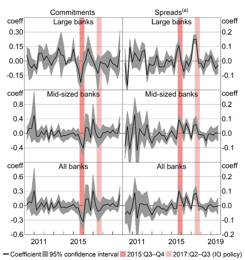
5.3 Heterogeneous effects
Specification (3) identifies the policy effect by estimating the difference in responses between banks
above and below the limit. The results do not show a clear effect with either measure of policy
treatment (Table 4). In the third and fourth quarters, investor commitments growth is indeed lower
for banks further above the limit (the column (a) coefficients are negative). However, the effect is
not statistically significant, and more broadly, the coefficient signs in columns (a) to (d) are not
consistent with the expected heterogeneous effect (negative for investor commitments, positive for
occupier commitments). Banks above the limit raise rates more than others in 2015:Q3 and Q4, but
roughly equally for targeted and non-targeted mortgages (columns (e) to (h)). The results provide
little indication that banks’ responses to the policy depend on their distance from the limit
(columns (a) to (c)) or whether they exceed the limit (columns (d) to (e)).
The lack of relationship between the policy treatment and changes in investor commitments growth
is visualised in Figure 5. In Q3 and Q4, most banks above the limit indeed reduce their investor
commitments growth, but this is also true for banks below the limit. This is consistent with the
unpredictability of conditions facing mid-sized banks that is discussed in Section 5.2. Mid-sized banks
below the limit, concerned about unpredictable flows pushing them above the limit, may have
reduced investor commitments as a precaution, including by raising investor rates.You can also read