Working Paper Series A dynamic model of bank behaviour under multiple regulatory constraints
←
→
Page content transcription
If your browser does not render page correctly, please read the page content below

Working Paper Series
              Markus Behn, Claudio Daminato,    A dynamic model of bank behaviour
                              Carmelo Salleo
                                                under multiple regulatory constraints

                                                   No 2233 / January 2019

Disclaimer: This paper should not be reported as representing the views of the European Central Bank
(ECB). The views expressed are those of the authors and do not necessarily reflect those of the ECB.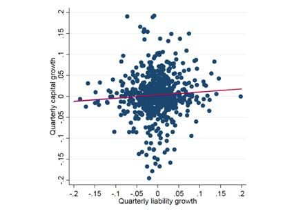
Abstract

      We develop a dynamic structural model of bank behaviour that provides a microeconomic
      foundation for bank capital and liquidity structures and analyses the effects of changes in
      regulatory capital and liquidity requirements as well as their interaction. Our findings suggest
      that adjustments in both types of requirements can have an impact on loan supply, with
      considerable heterogeneity across banks and over time. The model illustrates that banks’
      reactions depend on initial balance sheet conditions and reconciles evidence on short-term
      reductions in loan supply with findings suggesting that better capitalized banks are better
      able to lend in the medium- to long-term.
      Keywords: bank regulation, capital structure, liquidity structure, structural model
      JEL classification: G21, G28, G32

ECB Working Paper Series No 2233 / January 2019                                                          1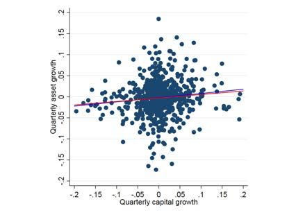
Non-technical summary

Following the global financial crisis of 2007-08, policy makers around the world have launched
a comprehensive reform programme aimed at increasing the banking sector’s resilience against
shocks. A key feature of this post-crisis regulatory framework is its multi-faceted nature, with
banks being subjected to multiple regulatory constraints aimed at capturing the various risk
dimensions on the solvency and liquidity side. Considering the variety of regulatory changes and
the relative novelty of many reform elements, assessing the joint impact of the adapted framework
on banks and the real economy is a challenging task for both regulators and academics.

    In this paper, we develop a dynamic partial equilibrium model of bank behavior that aims
at addressing these challenges by providing a microeconomic foundation for banks’ capital and
liquidity structures as well as their adjustments in response to regulatory changes and economic
shocks. The model takes a private perspective, which is justified by the observation that banks’
private adjustment decisions often transmit to the real economy via their impact on aggregate
loan supply. Moreover, the model features regulatory constraints on risk-weighted capital ratios
and liquidity ratios and is well suited for studying the interaction between these different types
of requirements.

    The stylized bank balance sheet in the model comprises loans and liquid assets on the as-
set side, and deposits, long- and short-term debt and equity on the liability side. Banks face
uncertainty with respect to assets returns, funding costs, and deposit volumes, and need to
consider various trade-offs simultaneously when taking decisions on how to adjust their balance
sheet structure. Generally, taking more risk allows them to generate higher expected returns,
while at the same time increasing the risk of breaching regulatory capital and/or liquidity re-
quirements or having to raise fresh equity in the market. The model accommodates potential
heterogeneity in banks’ response functions, reflecting the possibility that reactions may depend
on initial balance sheet conditions. This is important since different modes of adjustment may
have different social implications, for example with respect to the evolution of aggregate loan
supply and overall economic outcomes.

    We estimate the model on data for 116 institutions supervised by the European Single Su-
pervisory Mechanism (SSM), covering the quarters from 2014-Q1 to 2016-Q3 and containing
very granular balance sheet and income statement information. We estimate the structural
parameters of the model to match key balance sheet characteristics and dynamics observed in
the supervisory data. The estimated structural parameters provide an explanation for volun-
tary capital and liquidity buffers based on precautionary motives and confirm that regulatory
requirements are important determinants of actual capital and liquidity structures.

    The model suggests that changes in capital and liquidity requirements can have a material

ECB Working Paper Series No 2233 / January 2019                                                 2
impact on banks’ asset and liability structures and, consequently, aggregate lending in the
economy. In particular, the model predicts that most banks fully replenish their voluntary
buffers in response to increases in capital requirements, with considerable heterogeneity in the
mode of adjustment. This has important implications for the supply of loans. Generally, banks
that are initially more constrained (i.e., closer to the minimum capital requirement) choose
socially less desirable adjustment strategies, reducing loans considerably more than banks that
are initially less constrained. Moreover, our model suggests considerable differences between
transitory and medium- to long-term effects of higher capital requirements. While banks tend
to reduce loans in the short run, they also accumulate additional capital by retaining earnings,
which allows them to support lending at higher levels than before in the medium to long-run.

    We further show that also changes in liquidity requirements can have sizable real effects,
depending in particular on their interaction with capital requirements. Following an increase in
liquidity requirements banks react by holding a larger amount of liquid assets. Ceteris paribus,
increasing the amount of assets decreases capital ratios, so that further adjustments in the supply
of loans are necessary if banks wish to maintain constant voluntary capital buffers.

    This paper adds to the literature by proposing a novel methodology to study the dynamic
adjustment of bank capital and liquidity structures. Moreover, it contributes to the literature by
illustrating the trade-offs that banks need to consider in an environment with both capital and
liquidity requirements in a dynamic setting, and by offering insights on how capital and liquidity
requirements may interact to determine the response of banks to changes in either capital or
liquidity requirements.

    Our results reconcile empirical evidence on negative short-run effects of higher capital re-
quirements and positive long-run effects of higher bank capitalization. Moreover, they comple-
ment empirical evidence from the recent financial crisis showing that retaining earnings is the
preferred mode of adjusting to higher capital requirements. Overall, the results of the paper
highlight that the impact of changes in capital requirements, and in particular the short-term
lending reaction (which is often used as a proxy for the potential cost of policy measures), is
likely to depend on how binding the constraints are prior to the policy change.

ECB Working Paper Series No 2233 / January 2019                                                  3
1       Introduction

Following the global financial crisis of 2007-08, policy makers around the world have launched
a comprehensive reform programme aimed at increasing the banking sector’s resilience against
shocks. A key feature of this post-crisis regulatory framework is its multi-faceted nature, with
banks being subjected to multiple regulatory constraints aimed at capturing the various risk
dimensions on the solvency and liquidity side. Considering the variety of regulatory changes and
the relative novelty of many reform elements, assessing the joint impact of the adapted framework
on banks and the real economy is a challenging task for both regulators and academics (see, e.g.,
Financial Stability Board 2017). Existing models and empirical studies on regulatory impact
assessment often focus on the effects of higher capital requirements on lending, while there is little
evidence on the effects of liquidity regulation and the interaction of the various rules.1 Moreover,
empirical evidence on banks’ reactions is often limited to reduced form estimates that make it
difficult to foresee future adjustments (e.g., Aiyar et al. 2014, Behn et al. 2016b, Jiménez et al.
2017), and the theoretical banking literature has mainly been interested in normative, general
equilibrium considerations with respect to the optimal level of regulation (e.g., Diamond and
Rajan 2000, 2001, Admati and Hellwig 2013, DeAngelo and Stulz 2015).

    In this paper, we develop a dynamic partial equilibrium model of bank behavior that aims
at addressing these challenges by providing a microeconomic foundation for banks’ capital and
liquidity structures as well as their adjustments in response to regulatory changes and economic
shocks. The model takes a private perspective, which is justified by the observation that banks’
private adjustment decisions often transmit to the real economy via their impact on aggregate
loan supply. Moreover, the model features regulatory constraints on risk-weighted capital ratios
and liquidity ratios and is well suited for studying the interaction between these different types
of requirements.

    The stylized bank balance sheet in the model comprises loans and liquid assets on the asset
side, and deposits, long- and short-term debt and equity on the liability side. Banks face uncer-
tainty with respect to assets returns, funding costs, and deposit volumes, and need to consider
various trade-offs simultaneously when taking decisions on how to adjust their balance sheet
structure. Generally, taking more risk allows them to generate higher expected returns, while
at the same time increasing the risk of breaching regulatory capital and/or liquidity require-
ments or having to raise fresh equity in the market. To insure against profitability shocks on
the asset and/or funding side that can push capital ratios down, banks may hold additional
    1
     See, for instance, Berger et al. (2008), Flannery and Rangan (2008), Mehran and Thakor (2011), or Allen
et al. (2015). An early survey on the effects of capital requirements is provided by Thakor (1996). More recently,
some papers started to investigate how multiple constraints interact with each other (e.g., Cecchetti and Kashyap
2016, Chami et al. 2017, Goel et al. 2017, Mankart et al. 2018).

ECB Working Paper Series No 2233 / January 2019                                                                 4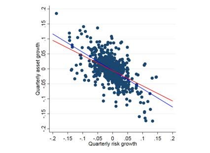
voluntary buffers on top of minimum capital requirements.2 A similar precautionary motive for
voluntary buffers arises on the liquidity side, where banks need to have a sufficient amount of
liquid assets to insure against possible outflows of deposits or fluctuations in liquid asset prices
or the cost of short-term debt. Our model provides an economic rationale for the magnitude
of these voluntary capital and liquidity buffers and thus provides insights on the importance of
precautionary motives in determining banks’ actual capital and liquidity structures.3 Moreover,
the rich characterisation of economic uncertainty, banks’ balance sheet structure and choices em-
bedded in the model allows analysing how capital and liquidity structures evolve over time, how
regulatory requirements interact with each other in shaping these dimensions, and how banks
adapt them in response to changes in capital or liquidity requirements. With respect to the
latter, the model accommodates potential heterogeneity in banks’ response functions, reflecting
the possibility that reactions may depend on initial balance sheet conditions. This is important
since different modes of adjustment may have different social implications, for example with
respect to the evolution of aggregate loan supply and overall economic outcomes.

    We estimate the model on data for 116 institutions supervised by the European Single
Supervisory Mechanism (SSM), covering the quarters from 2014-Q1 to 2016-Q3 and containing
very granular balance sheet and income statement information. Using a Simulated Method of
Moments approach, the model’s structural parameters are obtained by matching key balance
sheet characteristics and dynamics observed in the actual supervisory data. The estimated
structural parameters provide an explanation for voluntary capital and liquidity buffers based
on precautionary motives (see, e.g., Brunnermeier and Sannikov 2014 and Valencia 2014) and
confirm that regulatory requirements are important determinants of actual capital and liquidity
structures. Moreover, the estimates are consistent with frictions that prevent banks from freely
adjusting the amount of equity raised from external stakeholders. In line with the data, the
model suggests that asset expansion is mainly financed by debt issuance, while equity tends to
be relatively sticky, so that leverage is a major determinant of overall balance sheet size (see,
e.g., Adrian and Shin 2011). More specifically, increases in liquid assets tend to be financed
with short-term debt, while long-term debt and equity are more attractive when it comes to
financing loans. Moreover, asset expansions are associated with a decrease in average asset risk,
   2
     This precautionary motive for voluntary capital buffers is reminiscent of the models by Brunnermeier and
Sannikov (2014) and Valencia (2014). Valencia (2016) provides empirical evidence supporting such a motive.
   3
     A common view in the literature on bank capital structure is that holding capital imposes some kind of cost on
banks who consequently operate with capital ratios close to the regulatory minimum (e.g., Mishkin 2004, Van den
Heuvel 2008, Mehran and Thakor 2011, Allen et al. 2015, DeAngelo and Stulz 2015). In such a situation, even
small changes in requirements can have large implications for the structure of banks’ balance sheets and hence
the real economy. Contrasting with this view, recent empirical evidence shows that there is vast heterogeneity
in capital ratios, with many banks operating well-above the regulatory minimum (e.g., Flannery and Rangan
2008, Gropp and Heider 2010, Sorokina et al. 2017). This observation is consistent with papers arguing that the
Modigliani and Miller (1958) capital structure irrelevance theorem can be extended to banks (e.g., Miller 1995,
Admati et al. 2010, Kashyap et al. 2010, Admati and Hellwig 2013, Miles et al. 2013).

ECB Working Paper Series No 2233 / January 2019                                                                  5
which is consistent with banks targeting a risk-weighted capital ratio (see, e.g., Berger et al.
2008, Flannery and Rangan 2008) and the Value-at-Risk rule of equity management sketched
out in Adrian and Shin (2014). Finally, we observe a positive relation between changes in capital
and liquidity ratios, illustrating that specific adjustment actions such as reshuffling from loans
to liquid assets help to improve both ratios simultaneously.

    Using the estimated model, we simulate banks’ decisions under the actual economic and
institutional conditions during our sample period and then conduct a number of counterfactual
simulations to investigate how banks adjust asset and liability structures in response to policy
and economic shocks. The counterfactual simulations illustrate that changes in capital and
liquidity requirements can have a material impact on banks’ asset and liability structures and,
consequently, aggregate lending in the economy.

    The estimated model suggests that banks fully replenish their voluntary capital buffer in re-
sponse to changes in the minimum capital requirements (but go no further), in line with recent
empirical evidence provided by Bahaj and Malherbe (2017). At first glance, this seems to justify
the assumption of constant voluntary buffers that is often taken in models studying the relation
between bank capital and lending. However, our model illustrates that there is considerable
heterogeneity in the way in which banks move to higher capital ratios, with important impli-
cations for the supply of loans. Adjustments are achieved by a combination of accumulating
additional capital, reducing assets, and shifting from loans to liquid assets, where the overall
magnitude and the relative strength of these effects strongly depends on initial balance sheet
conditions of the bank as well as the time elapsed since the policy change. Generally, banks
that are initially more constrained (i.e., closer to the minimum capital requirement) choose so-
cially less desirable adjustment strategies, reducing loans considerably more than banks that
are initially less constrained. These results suggest that policy makers should account for initial
balance sheet conditions in the banking sector when implementing policy changes, instead of
assuming mechanical relations between capital regulation and lending. Moreover, our model
suggests considerable differences between transitory and medium- to long-term effects of higher
capital requirements. While banks tend to reduce loans in the short run, they also accumulate
additional capital by retaining earnings, which allows them to support lending at higher levels
than before in the medium to long-run. Thus, our paper dispels claims that higher capital re-
quirements will lead to permanent reductions in lending and reconciles empirical evidence on a
negative short-run impact of higher capital requirements and positive long-run effects of higher
capital ratios (e.g., Fraisse et al. 2015, Behn et al. 2016b, Jiménez et al. 2017 on the former, and
Gambacorta and Shin 2016 on the latter).

    We further show that also changes in liquidity requirements can have sizable real effects,
depending in particular on their interaction with capital requirements. Following an increase in
liquidity requirements banks react by holding a larger amount of liquid assets. Ceteris paribus,

ECB Working Paper Series No 2233 / January 2019                                                    6
increasing the amount of assets decreases capital ratios, so that further adjustments are nec-
essary if banks wish to maintain constant voluntary capital buffers.4 Our results show that
these adjustments can involve a reduction in loans, in particular for banks that are initially
more constrained by the liquidity requirement. Moreover, capital and liquidity ratios correlate
positively in general terms, and both capital and liquidity structures tend to become more stable
following changes in either requirement. However, banks generally compensate lower risk taking
on the asset side by taking more risk on the liability side, e.g. reducing the average maturity of
debt contracts. Consequently, under certain circumstances the decrease in solvency risk that is
usually associated with an increase in capital requirements may be accompanied by an increase
in liquidity risk, so that the aggregate impact on the riskiness of banks’ balance sheets depends
on the relative importance of solvency and liquidity risk. Overall, our results illustrate that
there are complex interactions between capital and liquidity regulations, and that a comprehen-
sive view on all dimensions is necessary in order to avoid potential unintended consequences of
regulatory policies.

    Our paper contributes to the literature by proposing a novel methodology to study the
dynamic adjustment of bank capital and liquidity structures. While the literature on liquidity
profiles is still scarce, previous papers studying the evolution of capital ratios have often used
partial adjustment models, assuming the existence of target capital structures towards which
banks adjust in case of deviations (see, e.g., Berger et al. 2008, Flannery and Rangan 2008, Gropp
and Heider 2010, Memmel and Raupach 2010, De Jonghe and Öztekin 2015). While the concept
is theoretically appealing, partial adjustment models are unable to distinguish between actual
targeting behaviour and mean reversion due to purely mechanical reasons (see Shyam-Sunder
and Myers 1999, Chen and Zhao 2007, Chang and Dasgupta 2009). The novel methodology
used in our paper avoids this pitfall and is able to identify actual targeting behaviour.

    In contrast to our model, theoretical papers on bank capital structure often focus on the
socially optimal level of bank capital, i.e. the capital structure of the bank that maximizes its
value for all stakeholders. Usually, the bank’s optimal capital structure trades off some kind of
bankruptcy cost against advantages of high leverage, due to agency problems (e.g., Diamond
and Rajan 2000, Acharya et al. 2016), compensation for liquidity production (e.g., DeAngelo
and Stulz 2015), tax benefits (e.g., Gornall and Strebulaev 2015, Sundaresan and Wang 2016),
the existence of deposit insurance (Allen et al. 2015), or simply the notion that equity is costly
for banks for various reasons (e.g., Mehran and Thakor 2011). A number of papers also consider
   4
     The result depends on the extent to which increasing the amount of liquid assets makes capital requirements
more binding. In reality, this is more likely to be the case for banks that are relatively more constrained by
the Leverage Ratio (i.e., an unweighted capital requirement). The reason for this is that liquid sovereign assets
carry a risk weight of zero percent in many jurisdiction and hence do not require any equity financing under the
risk-based framework, while they do enter the denominator and can thus increase the bindingness of the Leverage
Ratio.

ECB Working Paper Series No 2233 / January 2019                                                                7
the interaction between capital structure and asset risk (Shleifer and Vishny 1992, DeYoung
and Roland 2001, Greenlaw et al. 2008, Adrian and Shin 2010, 2014). In contrast to many of
these papers, we develop a positive dynamic model of bank adjustment behaviour, in which
banks determine their asset and liability structures based on private considerations (with social
implications).

    The paper also relates to studies on the relationship between bank capital or liquidity and
aggregate lending or real economic activity. One approach in this field is to use micro-level data
in order to identify how banks adjust lending behaviour in response to specific policy changes
or economic shocks (e.g., Peek and Rosengren 1997, Aiyar et al. 2014, Fraisse et al. 2015, Behn
et al. 2016b, Jiménez et al. 2017). Another approach is to investigate historical correlations
between fluctuations in bank capital and other variables of interest (e.g., Bernanke et al. 1991,
Hancock and Wilcox 1993, 1998, Berrospide and Edge 2010, Noss and Toffano 2016, Gross et al.
2016). Virtually all of these studies rely on reduced form estimates of past behaviour, which may
compromise their suitability for analysing the possible effects of future policy changes (see Lucas
1976). The structural nature of our model seeks to overcome this challenge, as it establishes
a microeconomic foundation for observed adjustments in capital and liquidity ratios and thus
allows deriving economically founded behavioural responses to changes in capital or liquidity
requirements.

    Finally, our paper adds to a small but growing literature studying the interaction of multiple
requirements in the post-crisis regulatory environment. Closely related is the paper by Mankart
et al. (2018), who develop a dynamic structural banking model to examine the interaction
between risk-weighted capital ratios and unweighted leverage requirements while abstracting
from the liquidity dimension. The same applies to Goel et al. (2017), who take a capital allocation
perspective and also study the interaction between risk-based capital requirements and a simple
leverage ratio. The interaction between Basel III type capital and liquidity requirements is
studied by Cecchetti and Kashyap (2016) and Chami et al. (2017). The former paper investigates
potential redundancy of different types of requirements, while the latter develops a dynamic
model for bank holding companies and studies how different types of investments on the asset
side interact with each other. Finally, a number of papers seek to assess the macroeconomic
effects of multiple constraints on bank capital and liquidity (e.g., Covas and Driscoll 2014,
Boissay and Collard 2016, Fender and Lewrick 2016). Our paper contributes to this literature
by illustrating the trade-offs that banks need to consider in an environment with both capital
and liquidity requirements in a dynamic setting, and by offering insights on how capital and
liquidity requirements may interact to determine the response of banks to changes in either
capital or liquidity requirements.

   The remainder of the paper is organized as follows: we develop our model in the next section
and describe the data set and estimation strategy in Section 3. Results of the estimation are

ECB Working Paper Series No 2233 / January 2019                                                  8
presented in Section 4, and results of the counterfactual simulation are shown in Section 5.
Finally, Section 6 concludes.

2     Model

We develop a dynamic stochastic model of bank behavior in the presence of economic uncertainty
and regulatory constraints on capital and liquidity ratios. The model allows to study how banks
take joint decisions with respect to asset growth, debt issuance, risk taking and payout policy,
this way providing a microeconomic foundation for the observed bank capital structures and
liquidity profiles and their dynamic adjustments. The following subsections include a description
of the model setup, the timing of events and decisions, the exogenous processes of the model,
the decision variables, the evolution of profits, the dynamics of capital and liquidity structures,
and banks’ dynamic optimization problem.

2.1    Model setup

The stylized bank balance sheet in our model is illustrated in Figure 1. It comprises two classes of
assets, loans and liquid assets, and four classes of liabilities, deposits, long- and short-term debt,
and equity. Decisions on how to adjust these asset and liability classes are taken by risk-neutral
managers in a discrete time, infinite horizon setting. These managers maximize shareholder
value in each period by jointly determining asset growth and structure, payout ratios (dividend
distribution and recapitalisation) and the financing mix between short-term and long-term debt,
while considering various trade-offs simultaneously. Taking more risks allows them to generate
higher expected returns, but comes at the risk of potentially larger shocks that may lead to a
deterioration in capital and liquidity ratios. Banks face regulatory requirements on both of these
ratios, and shareholders incur a cost in case the bank violates either type of requirement (or if the
bank decides to raise external equity in order to avoid breaching the capital requirement). Our
model features ex ante heterogeneity with respect to bank balance sheet size, asset composition
and liability structure. Heterogeneity in later periods also depends on the realization of shocks
on asset returns, cost of funding and volume of deposits.

2.2    The timing of events and decisions

The timing of events is illustrated in Figure 2. In each period, banks start with loans Lj,t ,
liquid assets Fj,t , equity Ej,t , deposits Dj,t , long-term debt LTj,t and short-term debt STj,t .
                                                                                           L and
Thereafter, banks take decisions on the payout policy divj,t , the issuance of new loans gj,t

ECB Working Paper Series No 2233 / January 2019                                                     9
LT , and the adjustment of liquid assets g F and short-term debt g ST . They
new long-term debt gj,t j,t j,t
take these decisions to maximize:
T
X
Et β s−t
divj,t+s − Ω × 1(CRj,t+s < θCR ) (1)
s=t
| {z } | {z }
future dividends cost of breaching capital requirements
− Ψ × 1(LRj,t+s < θLR ) − Φ1 (−divj,t+s ) × 1(divj,t+s < 0)
Φ2
| {z } | {z }
cost of breaching liquidity requirements cost of raising fresh equity
with β < 1 being the discount factor and Ts=t β s−t divj,t+s representing the stream of expected
P
future dividends. The remaining terms of the expression reflect the two types of frictions in
our model. First, the variables Ω and Ψ represent the costs of falling below regulatory capital
(θCR ) and liquidity requirements (θLR ). These costs are reminiscent of the bankruptcy cost in
classical trade-off theory models (see, for instance, Kraus and Litzenberger 1973 or Buser et al.
1981) and can be motivated by the risk for shareholders to be bailed in, possible restrictions on
dividend payments, or other supervisory measures that may be imposed in case of a breach of
requirements.5 Second, when raising fresh equity in the market (divj,t < 0) banks pay a cost
equal to φ1 (−divj,t+s )φ2 . These costs are meant to reflect the existence of direct transactional
costs and indirect costs of raising equity, e.g. related to debt overhang problems (Myers 1977,
Admati et al. 2012) or signaling costs (Myers and Majluf 1984). The assumption that raising
new external funds is costly is common in the banking literature (e.g., Greenwald et al. 1993,
Kashyap and Stein 1995, Froot and Stein 1998, Stein 1998, Valencia 2014) and consistent with
the observation that banks are often reluctant to tap the market for fresh equity. In line with
pecking order theory, the cost does not apply if banks decide to accumulate capital from retained
earnings. Importantly, both the costs of breaching minimum capital and liquidity requirements
and the cost of raising fresh equity are not imposed ex ante but estimated within our model
structure. Hence, our model allows to test both trade-off and pecking order theories, since a
zero value for either cost parameter would imply a rejection of the respective theory.
The structural parameters β, Ω, Ψ, Φ1 and Φ2 are crucial elements in determining banks’
adjustment functions and are estimated making use of the economic model (see Section 3.2).
Given the structural parameters, the evolution of balance sheets depends on banks’ decisions
L , g F , g LT , g ST ) and realized profits. Profits, in turn, depend on banks’ decisions
Γj,t = (divj,t , gj,t j,t j,t j,t
and the realization of shocks on asset returns, cost of funding, and the volume of deposits (see
next subsection).
5
Our model abstracts from potential agency problems between bank managers and shareholders. However,
breaching requirements may also have personal consequences for managers who could be removed in such case.
ECB Working Paper Series No 2233 / January 2019 102.3 Exogenous processes
A key determinant of banks’ choices with respect to asset and liability structure is the uncertainty
they face with respect to returns on loans and liquid assets, prices of liquid assets and interest
rates on long- and short-term debt. We assume that price processes on the asset and liability
side are exogenously determined, i.e. banks are price takers whose decisions do not have any
impact on asset returns. That is, rates on loans and liquid assets are determined in competitive
markets, and banks can (up to a certain limit) expand their lending at the prevailing market
rates. This assumption is justified by the short- to medium perspective taken by our partial
equilibrium model: while one would expect some interaction between loan volumes and interest
rates in a long-term general equilibrium framework, we think that it is unlikely that banks
account for such long-run effects in their short-term adjustment decisions.
Specifically, returns on loans and liquid assets for bank j at time t evolve according to the
following simple processes:
L
rj,t = rtCB + µ − ζ + ηj,t
rL rL
with ηj,t 2
∼ N (0, σrL ) (2)
F
rj,t = rtCB + rF
+ ηj,t rF
with ηj,t 2
∼ N (0, σrF ) (3)
where rtCB is the interest rate set by the central bank, µ the constant mark-up charged by
banks on loans in an oligopolistic market, ζ the expected impairment rate on loans, and ηj,t rL
a conditionally homoskedastic normally, independently and identically distributed (i.i.d.) error
with variance σrL2 that reflects the non-diversifiable component of risk in the loan portfolio.
Heterogeneity with respect to banks’ returns on loans then comes from the idiosyncrasy of
shocks in each period, which can be interpreted as exogenous economic shocks hitting local
rF is a
economies in different ways. For liquid assets, ψ reflects the average risk premium and ηi,t
2 . We expect that (µ − ζ) > ψ and σ 2 > σ 2 , since loans
normally i.i.d. error with variance σrF L rF
are typically more profitable but also more risky than liquid assets.
The prices of liquid assets are assumed to evolve following a unit root model:
F F pF pF 2
ln Pj,t+1 = ln Pj,t + ηj,t with ηj,t ∼ N (0, σpF ) (4)
The price process for liquid assets is bank-specific, to capture different compositions of the
pF
trading book across banks. The shock ηj,t is a conditionally homoskedastic normally i.i.d.
2
error with variance σpF which directly affects banks’ asset values, profits, and both capital and
liquidity ratios. For the covariance between shocks to asset prices and returns we assume that
σrF,pF = −1, reflecting the usual inverse relationship between asset prices and returns.
For interest rates on deposits, long-term debt, and short-term debt, we assume:
iD CB
t = rt +φ (5)
ECB Working Paper Series No 2233 / January 2019 11iLT CB
j,t = rt + ξ + κLT LEVj,t + ηj,t
iL iL
with ηj,t 2
∼ N (0, σiL ) (6)
iST CB
j,t = rt + γ + κST LEVj,t + ηj,t
iS iS
with ηj,t 2
∼ N (0, σiS ) (7)
In line with the sticky nature of deposits, the deposit rate iD t depends only on the interest
rate set by the central bank and a constant mark-up φ, determined in oligopolistic competition
among banks. In contrast, interest rates on long-term debt and short-term debt are subject to
uncertainty, i.e. conditionally homoskedastic normally i.i.d. shocks in each period. In addition
to the general mark-ups ξ and γ, we allow the cost of both long and short-term debt to depend
on the bank’s leverage, reflecting the idea that higher levels of equity financing should generally
lower the bank’s cost of funding (see, e.g., Admati et al. 2010).6 We expect short-term debt to
be generally cheaper than long-term debt (ξ + κLT LEVj,t > γ + κST LEVj,t ), while short-term
2 < σ 2 ). Moreover, the distribution for the interest
rates are subject to larger fluctuations (σiL iS
rate on short-term debt includes an event corresponding to a tenfold increase in interest rates,
occurring with a one percent probability, which reflects the idea of a possible run on short-term
debt.
The exogenous shocks are collected in the vector Hj,t = (ηj,t rL , η rF , η pF η iS , η iL , η D ). As
j,t j,t j,t j,t j,t
mentioned, we assume that the shock variances Σ = (σrL 2 , σ 2 , σ 2 , σ 2 , σ 2 , σ 2 ) as well as the
rF pF iL iS D
parameters µ, ψ, φ, ξ, κLT , γ, and κST are exogenous financial factors which we estimate directly
from the data. In contrast, we estimate banks’ expectations with respect to the future impair-
ment rate on loans, captured by ζ, by making use of the model as described in Section 3.2.
Deriving ζ endogenously within the model structure rather than using realized (ex-post) im-
pairment rates as a proxy is motivated by the idea that expectations with respect to future
impairment rates may differ from realized rates in the past, so that it is preferable to infer the
value of expected default rates implied by banks’ observed lending behavior.
2.4 Choices on the adjustment of assets and liabilities
Besides the evolution of the exogenous stochastic processes described in the previous section,
banks’ profits in each period depend on the choices they make with respect to the adjustment
of assets and liabilities. As mentioned before, banks’ choices are entirely based on private
considerations, reflecting the positive nature of our model. In particular, banks take decisions
in order to maximize the stream of expected future dividends, i.e. shareholder value. At the
same time, they want to avoid breaching regulatory requirements or having to raise fresh equity,
which gives rise to the model’s basic trade-off: while taking more risk allows generating higher
expected returns, it comes at the cost of higher uncertainty with respect to solvency or liquidity
6
Our model does not feature government bailouts, consistent with the intention of post-crisis resolution reforms
to address too-big-to-fail (TBTF) problems in the banking sector. Therefore, considerations related to potential
TBTF subsidies are not part of the trade-offs which banks face when maximizing profits.
ECB Working Paper Series No 2233 / January 2019 12positions and thus increases the risk of breaching regulatory requirements or having to raise
fresh equity. As a result of this trade-off banks may want to hold precautionary capital and
liquidity buffers on top of their minimum requirements, where the evolution and the adjustment
of these precautionary buffers in response to regulatory or economic shocks is at the core of our
interest.
Asset structure We assume that loans are sticky and illiquid assets that evolve according to
the following equation:
1 L L
Lj,t+1 = Lj,t (1 − + gj,t ) with gj,t ∈ [0, gtL ] (8)
mL
with mL being the average loan maturity and gj,t
L the fraction of new loans being issued in period
t. We assume that loans remain in the banks’ balance sheet until the original principal is repaid.
The amount being repaid in each period is equal to the inverse of the average maturity mL and
constitutes the maximum possible decrease in the stock of loans in period t (assuming gj,tL = 0).
On the other side, the maximum increase in the stock of loans is given by − m1L + gj,t
L.
Liquid assets evolve as follows:
F F
Fj,t+1 = Fj,t (1 + gj,t ) with gj,t ∈ [gtF , gtF ] (9)
F is the adjustment in liquid assets. By definition, liquid assets can always be sold at
where gj,t
prevailing market prices, which is why their adjustment does not depend on their maturity and
is hence more flexible than the adjustment of the stock of loans.
When deciding on the adjustment of loans and liquid assets, banks need to consider that
loans typically generate higher expected returns (since (µ − ζ) > ψ) that are, however, also
more volatile (since σL2 > σrF2 ). Thus, increasing the fraction of loans implies higher expected
profitability, but also increases the risk of breaching regulatory capital requirements. At the
same time, there is an interaction with the bank’s liability structure, at least partly due to
regulation. As we will discuss below, reshuffling from loans to liquid assets can help to improve
both capital and liquidity ratios, since liquid assets are treated more favourably in both types
of regulations. To the extent that constraints on these ratios are binding, liquid assets will have
a funding advantage relative to loans, since they require less equity financing (due to the lower
risk weights) and can more easily be financed by using cheaper short-term debt (due to the
definition of the liquidity ratio). That is, while loans generate higher expected returns they are
usually financed with lower (and more expensive) leverage, which ensures that both loans and
liquid assets are attractive from an investment standpoint.
Debt structure Besides equity, banks finance their activities through deposits collected from
households and non-financial corporations, long-term debt with maturity mLT and short-term
ECB Working Paper Series No 2233 / January 2019 13debt that needs to be rolled over in each period. By distinguishing three forms of debt with
different characteristics we go beyond the traditional banking literature that often focuses on
the transformation of deposits into loans (e.g., Diamond and Dybvig 1983, Diamond and Rajan
2000, 2001, Kashyap et al. 2002). This extension enables us to study the interaction of banks’
overall financing choices with asset composition and profitability.
Long-term debt and short-term debt evolve according to the following equations:
1 LT LT
LTj,t+1 = LTj,t (1 − + gj,t ) with gj,t ∈ [0, gtLT ] (10)
mLT
ST ST
STj,t+1 = STj,t (1 + gj,t ) with gj,t ∈ [gtST , gtST ] (11)
with mLT and gj,t
LT being the average maturity and the new issuance of long-term debt, and
ST the adjustment in short-term debt. As for loans, using long-term debt introduces a rigidity
gj,t
in banks’ balance sheets, with the maximum reduction in long-term debt being limited by the
amount arriving at maturity ( m1LT ). In contrast, short-term debt needs to be rolled over each
period and can hence be adjusted more flexibly.
A higher share of long-term debt is associated with higher interest expenses (since ξ +
κLT LEVj,t > γ +κST LEVj,t )), but provides insurance against future shocks to funding costs and
the risk of a run on short-term debt (i.e., a sharp increase in short-term debt rates). Moreover,
loans can be financed with short-term debt only to a limited extent, since liquidity requirements
limit the amount of maturity transformation that banks can engage in. Hence, if banks want
to expand the relatively more profitable loans they need to rely on long-term debt or equity
financing.
We assume that deposits from households and non-financial corporations are determined
exogenously. That is, similarly to Kashyap and Stein (1995), we do not allow for interbank
competition for deposits from households and non-financial corporations, but assume that fluc-
tuations in such deposits are entirely exogenous. The reason for taking this assumption is that
price competition for deposits is a long-term process, so that it is not possible for banks to
simply adjust the amount of deposits in the short- to medium-term. Hence, if banks want to
leverage up or down by taking additional debt, they need to rely on short- or long-term whole-
sale funding, consistently with the results in Adrian and Shin (2010, 2014) and in line with the
sticky nature of deposits. Nevertheless, the volume of deposits is subject to exogenous shocks,
to capture the idea that a fraction of depositors may want to extract their money in each period.
This is an important source of liquidity risk in the model, and bank managers may decide to
insure against such risk by holding a sufficient amount of liquid assets. Deposits are assumed to
evolve according to the simple dynamic equation:
D D 2
Dj,t+1 = Dj,t + ηj,t with ηj,t ∼ N (0, σD ) (12)
D is an normally i.i.d. distributed idiosyncratic shock with variance σ 2 . The existence of
where ηj,t D
ECB Working Paper Series No 2233 / January 2019 14D reflects the risk of a run on deposits and forms part of the motivation for liquidity
the shocks ηj,t
regulation in our model (besides the possibility of rollover problems for short-term debt). As
such, our model relates to the classical banking literature cited above, in which fragile deposits
give rise to potential liquidity problems for the bank.
2.5 The profit function and budget constraint
Bank profits at time t + 1 depend on a set of exogenous parameters (rtCB , µ, ψ, φ, ξ, κLT , γ,
κST ), the expected impairment rate on loans (ζ), the realization of the shocks Hj,t , and banks’
choices Γj,t . End-of-period profits of bank j can be written as:
L F pF
Πj,t+1 = rj,t+1 Lj,t+1 + rj,t+1 Fj,t+1 + ηj,t Fj,t (13)
| {z } | {z }
return on loans return on liquid assets
CB 1
− (rt+1 + ξ)LTj,t (1 − LT ) − iLT LT
j,t+1 gt LTj,t
| {z m } | {z }
cost of existing long-term debt cost of new long-term debt
− iST
j,t+1 STj,t+1 − iD Dj,t+1 − exp(ι1 + ι2 × log(Aj,t ))
| {z } |t+1 {z } | {z }
cost of short-term debt cost of deposits operating cost
where the last term is an operating cost associated with banking activity (capturing administra-
tive expenses and amortization of physical capital, net of net fee and commission income) that
is defined in exponential terms to allow for possible economies of scale, and the other variables
are defined in the previous sections. Banks’ income arises from stochastic returns on loans and
liquid assets, while changes in liquid asset prices can exert either positive or negative effects
on profits. Banks have to pay interest rates on long-term debt, short-term debt and deposits,
where all of the short-term debt and the newly issued long-term debt are subject to an interest
rate shock.
The budget constraint is defined by banks’ balance sheet structure and can be described in
terms of the asset evolution equation:
Aj,t+1 = Aj,t + Πj,t+1 − divj,t + ∆Dj,t+1 + ∆LTj,t+1 + ∆STj,t+1 (14)
where ∆Xt+1 is the variation in variable X between beginning and end of period (∆Xj,t+1 =
Xj,t+1 − Xj,t ). The equation ensures that the balance sheet identity is met in each period,
since changes in assets are determined by the sum of retained earnings and changes in debt, i.e.
ECB Working Paper Series No 2233 / January 2019 15changes in assets are equal to changes in aggregate liabilities.7
2.6 Dynamics of capital and liquidity structures
Capital structure The focus of our analysis is on how banks’ decisions on asset growth, debt
issuance, risk taking and payout policy jointly determine the evolution of capital and liquidity
structures. Bank equity evolves according to the following equation:
Ej,t+1 = Ej,t + Πj,t+1 − divj,t (15)
The equation illustrates that capital can be accumulated by retaining earnings (divj,t < Πj,t+1 )
and by raising fresh equity (divj,t < 0). Banks’ decision to accumulate capital depends on
the discount factor β (capturing the impatience of stockholders), the expected return on capital
(depending on the choice of the balance sheet structure and the exogenous parameters controlling
the profit function), the level of uncertainty about future profits (reflected in the size of the shock
variances, and impacting the precautionary motive for capital accumulation), the regulatory
costs associated with capital falling below the minimum requirement, and the cost associated
with raising equity externally.
The minimum capital requirement is defined in terms of risk-weighted assets, in line with the
idea that riskier assets should be subject to higher capital requirements (see Basel Committee on
Banking Supervision 2010). In our simplified framework, the evolution of risk weights is defined
as follow:
Lj,t+1 Fj,t+1
RWj,t+1 = wL + wF + wO Aj,t+1 (16)
Aj,t+1 Aj,t+1
where wL and wF are the average risk weights associated with loans and liquid assets, and wO
is a risk weight for operational risk that is assumed to be proportional to total assets.8 As
mentioned, we expect loans to be riskier than liquid assets, and hence wL > wF .
Eqs. 13 to 16 contain the major factors affecting the evolution of the risk-weighted capital
ratio, which depends on the realization of the shocks collected in Hj,t and banks’ joint decisions
7
In practice, to ensure that the balance sheet identity holds at each point in time, one of the variables on
the asset or liability side needs to be treated as a residual, the evolution of which is implied by the evolution of
the other variables. For the solution of the model, we treat liquid assets as the residual variable. In particular,
the model specification allows to trivially recover the amount of next-period liquid assets Fj,t+1 as the difference
between end-of-period total assets and loans: Fj,t+1 = Aj,t+1 − Lj,t+1 , where end-of period total assets and loans
are determined as specified in Eqs. 14 and 8, respectively.
8
Risk weights for operational risk are included for the sake of completeness (see Basel Committee on Banking
Supervision 2010) and to ensure consistency between the aggregate risk exposure amount generated by our model
and that observed in the data.
ECB Working Paper Series No 2233 / January 2019 16with respect to the adjustment of assets and liabilities collected in Γj,t . Specifically, the risk-
weighted capital ratio evolves as follows:
Ej,t+1
CRj,t+1 = (17)
RWj,t+1 Aj,t+1
The equation illustrates that banks have at least four different modes of adjustment to increase
the risk-weighted capital ratio (compare with Adrian and Shin 2010, Admati et al. 2012): (i) by
using new equity (raised in the market or from retained earnings) to buy back debt, while keeping
assets constant (Et ↑, At →), (ii) by using new equity to fund asset growth, while keeping debt
constant (Et = At > 0), (iii) by selling assets and using the proceeds to buy back debt, while
keeping equity constant (At ↓, Et →), and (iv) by reshuffling assets towards less risky activities
(thus decreasing average risk weights in the portfolios), while keeping assets and equity constant
(RWt ↓, Et →, At →). Hence, banks have several levers to manage their capital structure, and
decisions on these levers are likely to interact with each other. Furthermore, the different modes
of adjustment are likely to have different macroeconomic implications. For example, effects on
lending and the real economy could be particularly pronounced under modes (iii) and (iv), where
banks reduce the amount of loans in order to reduce debt or to invest more funds into less risky
assets. A main contribution of our paper is hence to illustrate the importance of the different
modes of adjustment under different initial conditions, which should help gauging the possible
impact of proposed policy measures.
Liquidity structure The end-of-period liquidity ratio is given by:
Fj,t+1
LRj,t+1 = (18)
wST × STj,t+1 + wD × Dj,t+1
Although simplified, the liquidity requirement in our model resembles the Basel III Liquidity
Coverage Ratio (LCR) that is meant to ensure that financial institutions have a sufficient amount
of liquid assets to be able to withstand short-term liquidity disruptions.9 The weights wST and
wD specify the fraction of the respective liability class that needs to be covered with liquid
assets. Deposits are generally more stable than other short-term debt, so that wST > wD
(since long-term debt has a pre-defined maturity it cannot be withdrawn under stress, so that
wLT = 0). Similar to the capital ratio, the evolution of the liquidity ratio depends on both
banks’ adjustment decisions and the realization of the shocks. The formula illustrates that
banks have two possibilities to improve their liquidity ratio: (i) by increasing the amount of
liquid assets (Ft ↑); and (ii) by decreasing the amount of short-term debt (STt ↓; recall that
deposits are exogenous and hence not a choice variable of the bank). Again, the different modes
of adjustment could have different implications from a social perspective, and we will investigate
this further in Section 5.
9
The Basel III Liquidity Coverage Ratio is defined as the ratio between the stock of High Quality Liquid Assets
and total net cash outflows under stressed conditions over a period of 30 days (see Basel Committee on Banking
Supervision 2013 for details).
ECB Working Paper Series No 2233 / January 2019 17Capital and liquidity regulation Finally, the institutional framework is characterised by
the presence of minimum risk-weighted capital requirements θCR and liquidity requirements θLR .
The regulatory requirements are such that CRj,t+1 > θCR and LRj,t+1 > θLR ∀j = 1, ...J and
t = 0, ...T −1. As specified in Eq. 1, banks face costs Ω and/or Ψ when breaching these regulatory
requirements. The introduction of costs associated with the violation of regulatory requirements,
in a context with uncertainty and credible liability and asset structures, allows to investigate the
role of regulation in the evolution of capital and liquidity profiles. In particular, we test whether
and how much regulatory requirements are indeed important determinants of banks’ capital
and liquidity profiles by estimating the values of Ω and Ψ: a rejection of the null hypothesis
of Ω (or Ψ) equal to zero would indicate that minimum requirements are indeed an important
factor for banks’ decisions on capital and liquidity profiles. In particular, the interplay between
profitability, the cost of equity, the level of uncertainty and the costs of breaching regulatory
requirements shapes banks’ decisions and induces optimal buffers held on top of either minimum
requirement in order to insure against possible shocks. Generally, these buffers can be expected
to be larger the larger costs of breaching capital and liquidity requirements. Moreover, positive
parameter values for Ω and Ψ would be consistent with classical trade-off theories of capital
structure, since the cost of breaching regulatory requirements are reminiscent of the bankruptcy
cost usually included in such models.
2.7 Banks dynamic programming problem and solution of the model
The evolution of the entire balance sheet structure can be pinned down by means of five state
variables, collected in the vector Θj,t = (CRj,t , CRj,t , Ej,t , LAj,t , DLj,t ). The state variables
are the capital and liquidity ratios, the level of equity capital, the share of loans in total assets
LAj,t = Lj,t /Aj,t , and the share of deposits in total debt DLj,t = Dj,t /(Dj,t + LTj,t + STj,t ).
The solution of our model derives banks’ optimal decisions Γj,t for each point of the state space,
so that we can disentangle the relevance of different modes of adjustment for different balance
sheet conditions.
Besides the state of the system, optimal decisions at each point in time depend on the
exogenous financial factors determining the data generating process for the stochastic variables
(rtCB , µ, ψ, φ, ξ, κLT , γ, κST and Σ) and the remaining structural parameters β, Ω, Ψ, Φ1 ,
Φ2 and ζ. In each period t, banks start with loans and liquid assets funded by equity, deposits,
long-term and short-term debt from time t − 1, and receive profits from banking activity as
described in Eq. 13.
In this set up, the dynamic optimization problem can be written as:
Vj,t (Θj,t ) = max divj,t −Ω × 1(CRj,t+s < θCR ) (19)
Γj,t
ECB Working Paper Series No 2233 / January 2019 18
          −Ψ × 1(LRj,t+s < θLR ) − Φ1 (−divj,t+s )    Φ2
                                                           × 1(divj,t+s   < 0) + β Et Vj,t+1 (Θj,t+1 )

subject to the constraints listed in Eqs. (2) to (18) and the definition of the state variables.

    The problem cannot be solved analytically. Instead, we derive optimal decisions at each point
of the state space via backward induction, using a standard value function iteration approach.
That is, we assume that banks will be liquidated in some future period T (we set T = 100),
paying out the entire equity in that period without taking any other decisions. Given the
value function obtained for period T , we can compute optimal decisions in previous periods. In
particular, optimal decisions for each point of the state space in period T − 1 are determined
such that they maximize the value function of the bank. Going back in time, this procedure is
repeated until the policy functions converge.10

     To solve the model we need to discretize the state variables Θj,t and and the choice variables
Γj,t , which we do by using an exponential grid for capital and equally spaced grids for the
remaining variables (see Appendix Table A.1 for the exact parametrization). To account for the
stochastic nature of the model, we take expectations with respect to the shocks on asset returns,
cost of funding, and deposit volumes when deriving optimal decisions at each point of the state
space. The density functions for the shocks are approximated, following Tauchen (1986), using
gaussian quadrature method when performing the numerical integrations. Finally, we use linear
interpolations to evaluate next-period’s value function for values of the state variables that do
not lie on the exogenous predefined grids.

3        Data and estimation strategy

We solve the the model numerically by making use of granular supervisory data on bank balance
sheets and income statements. This section describes our data set and estimation strategy and
reports results for some standard capital and liquidity structure regressions.

3.1      Data

The data we use to estimate the model includes information on 116 institutions supervised by the
European Single Supervisory Mechanism (SSM), covering the quarters from 2014-Q1 to 2016-
Q3 and containing very granular balance sheet and income statement information. Descriptive
statistics for the data are presented in Table 1, and a description of all variables is available in
    10
     That is, we solve the model backwards for 100 periods and check that the policy functions have converged,
i.e. ||Γt (Θ) − Γt−1 (Θ)|| = 0.

ECB Working Paper Series No 2233 / January 2019                                                            19
Appendix Table A.2. Banks in our sample are rather large, with average assets of more than
e200 billion, which is in line with their status as SSM significant institutions.11 As expected,
the risk-weighted capital ratio is on average considerably higher than the unweighted capital
ratio, reflecting the average ratio of risk-weighted assets to assets of 45 percent. We report two
different values for the liquidity ratio: the first one is the actual Basel III Liquidity Coverage
Ratio (LCR) as reported by the banks, while the second is a proxy variable that we calculate in
order to match the definition of the liquidity ratio in our model as specified in Eq. 18 (see below
for details on the calculation). The distributional characteristics of the two ratios are close to
each other, making us confident that we have obtained a good proxy. The table further shows
that profitability of European banks is rather low throughout the sample period, with the average
quarterly return on assets being only slightly above zero. Finally, it includes a breakdown of
assets and liabilities by counterparty: Exposures to corporates and households each account for
roughly a quarter of the average bank’s assets, with the government sector being the third most
important sector. On the liability side, households are by far the largest counterparty, although
the fraction of instruments with no specific counterparty (inter alia including debt securities
issued, capital and subordinated liabilities, and derivatives) is sizable.
3.2 Estimation strategy
This subsection presents the strategy we use to estimate the structural parameters of the model.
The parameters are estimated such that the model describes a number of key features of banks’
behavior with respect to the level and the adjustment of their (risk-weighted) capital and liquid-
ity structures. We use a two-step strategy similar to that employed, among others, in Gourinchas
and Parker (2002). In the first step, the parameters and functions characterising the exogenous
stochastic processes in the model (rtCB , µ, ψ, φ, ξ, κLT , γ, κST , and Σ) are estimated directly
from quarterly supervisory data. In the second step, we estimate the remaining structural pa-
rameters (β, Φ1 , Φ2 , Ω, Ψ, and ζ) by targeting empirical moments characterizing the dynamic
behavior of banks in our data, taking as given the values of the exogenous parameters estimated
in the first step.
Exogenous parameters The supervisory data contain detailed balance sheet information
that allow us to estimate the parameters characterising the profit function. These are key
ingredients to our analysis and reflect on the financial conditions which banks face over the
sample period. The data include detailed information on the items that compose the statement
11
According to the SSM Framework Regulation, all institutions with total assets larger than e30 billion are
considered significant. Moreover, institutions are considered significant if their assets exceed 20 percent of national
GDP, if they are one of the three largest credit institutions in a country, if they receive direct assistance from the
European Stability Mechanism, or if they have significant cross-border activities.
ECB Working Paper Series No 2233 / January 2019 20You can also read