IntelliO3-ts v1.0: a neural network approach to predict near-surface ozone concentrations in Germany - GMD
←
→
Page content transcription
If your browser does not render page correctly, please read the page content below
Geosci. Model Dev., 14, 1–25, 2021
https://doi.org/10.5194/gmd-14-1-2021
© Author(s) 2021. This work is distributed under
the Creative Commons Attribution 4.0 License.

IntelliO3-ts v1.0: a neural network approach to predict near-surface
ozone concentrations in Germany
Felix Kleinert1,2 , Lukas H. Leufen1,2 , and Martin G. Schultz1
1 Jülich   Supercomputing Centre, Forschungszentrum Jülich, Jülich, Germany
2 Institute  of Geosciences, Rheinische Friedrich-Wilhelms-Universität Bonn, Bonn, Germany

Correspondence: Felix Kleinert (f.kleinert@fz-juelich.de)

Received: 3 June 2020 – Discussion started: 17 August 2020
Revised: 6 November 2020 – Accepted: 7 November 2020 – Published: 4 January 2021

Abstract. The prediction of near-surface ozone concentra-         1   Introduction
tions is important for supporting regulatory procedures for
the protection of humans from high exposure to air pol-
lution. In this study, we introduce a data-driven forecast-       Exposure to ambient air pollutants such as ozone (O3 ) is
ing model named “IntelliO3-ts”, which consists of multi-          harmful for living beings (WHO, 2013; Bell et al., 2014;
ple convolutional neural network (CNN) layers, grouped to-        Lefohn et al., 2017; Fleming et al., 2018) and certain crops
gether as inception blocks. The model is trained with mea-        (Avnery et al., 2011; Mills et al., 2018). Therefore, the pre-
sured multi-year ozone and nitrogen oxide concentrations of       diction of ozone concentrations is of major importance for
more than 300 German measurement stations in rural envi-          issuing warnings for the public if high ozone concentrations
ronments and six meteorological variables from the meteo-         are foreseeable. As tropospheric ozone is a secondary air pol-
rological COSMO reanalysis. This is by far the most exten-        lutant, there is nearly no source of directly emitted ozone. In-
sive dataset used for time series predictions based on neural     stead, it is formed in chemical reactions of several precursors
networks so far. IntelliO3-ts allows the prediction of daily      like nitrogen oxides (NOx ) or volatile organic compounds
maximum 8 h average (dma8eu) ozone concentrations for             (VOCs). Weather conditions (temperature, irradiation, hu-
a lead time of up to 4 d, and we show that the model out-         midity, and winds) have a major influence on the rates of
performs standard reference models like persistence models.       ozone formation and destruction. Ozone has a “chemical life-
Moreover, we demonstrate that IntelliO3-ts outperforms cli-       time” in the lower atmosphere of several days and can there-
matological reference models for the first 2 d, while it does     fore be transported over distances of several hundred kilome-
not add any genuine value for longer lead times. We attribute     tres.
this to the limited deterministic information that is contained      Ozone concentrations can be forecasted by various nu-
in the single-station time series training data. We applied a     merical methods. Chemical transport models (CTMs) solve
bootstrapping technique to analyse the influence of different     chemical and physical equations explicitly (for example,
input variables and found that the previous-day ozone con-        Collins et al., 1997; Wang et al., 1998a, b; Horowitz et al.,
centrations are of major importance, followed by 2 m tem-         2003; von Kuhlmann et al., 2003; Grell et al., 2005; Don-
perature. As we did not use any geographic information to         ner et al., 2011). These numerical models predict concentra-
train IntelliO3-ts in its current version and included no re-     tions for grid cells, which are assumed to be representative
lation between stations, the influence of the horizontal wind     of a given area. Therefore, local fluctuations which are be-
components on the model performance is minimal. We ex-            low model resolution cannot be simulated. Moreover, CTMs
pect that the inclusion of advection–diffusion terms in the       often have a bias in concentrations, turnover rates, or meteo-
model could improve results in future versions of our model.      rological properties which have a direct influence on chemi-
                                                                  cal processes (Vautard, 2012; Brunner et al., 2015).
                                                                     This makes CTMs unsuited for regulatory purposes, which
                                                                  by law are bound to station measurements, except if so-called

Published by Copernicus Publications on behalf of the European Geosciences Union.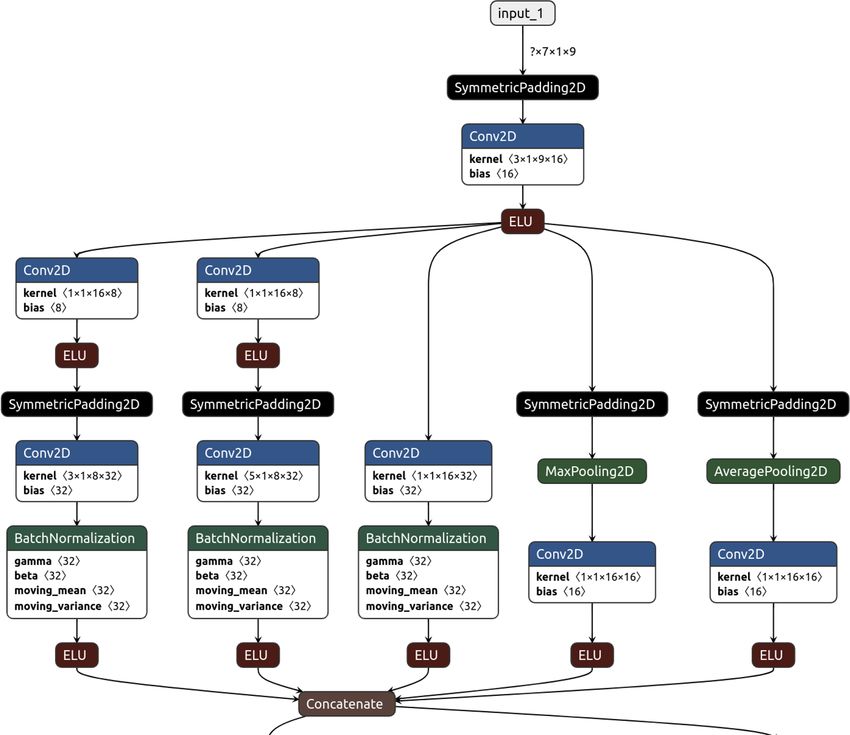
2                                                                                               F. Kleinert et al.: IntelliO3-ts v1.0

model output statistics are applied to the numerical mod-           stations (data range from 2008 to 2009). We evaluate the per-
elling results (Fuentes and Raftery, 2005). As an alterna-          formance at 203 stations, which have data during the 2010–
tive to CTMs, regression models are often used to generate          2015 period looking at skill scores, the joint distribution of
point forecasts (for example, Olszyna et al., 1997; Thomp-          forecasts and observations, as well as the influence of input
son et al., 2001; Abdul-Wahab et al., 2005). Regression mod-        variables.
els are pure statistical models, which are based on empirical          This article is structured as follows: in Sect. 2, we explain
relations among different variables. They usually describe a        our variable selection and present our prepossessing steps.
linear functional relationship between various factors (pre-        In Sect. 3, we introduce our forecasting model (IntelliO3-
cursor concentrations, meteorological, and site information)        ts, version 1.0). Section 4 introduces the statistical tools and
and the air pollutant in question.                                  reference models which were used for verification. In Sect. 5,
   Since the late 1990s, machine learning techniques in the         we present and discuss the results and analyse the influence
form of neural networks have also been applied as a regres-         of different input variables on the model performance. In
sion technique to forecast ozone concentrations or thresh-          Sect. 6, we discuss the limitations of IntelliO3-ts. Finally,
old value exceedances (see Table 1). As the computational           Sect. 7 provides conclusions.
power was limited in the early days of those approaches,
many of these early studies focused on a small number of
measurement stations and used a fully connected (FC) net-           2     Variable selection and data processing
work architecture. More recent studies explored the use of
                                                                    2.1    Variable selection
more advanced network architectures like convolutional neu-
ral networks (CNNs) or long short-term memory (LSTM)                Tropospheric ozone (O3 ) is a greenhouse gas formed in the
networks. These networks were also applied to a larger num-         atmosphere by chemical reactions of other directly emitted
ber of stations compared to the earlier studies and some stud-      pollutants (ozone precursors) and therefore referred to as a
ies have tried to generalise, i.e. to train one neural network      secondary air pollutant.
for all stations instead of training individual networks for          The continuity equation of near-surface ozone in a specific
individual stations (Table 1). Although the total number of         volume of air can be written as (Jacobson, 2005, p. 74ff)
studies focusing on air quality or explicit near-surface ozone
is already quite substantial, there are only few studies which      ∂Nq
                                                                        + ∇ · vNq = (∇ · Kh ∇) Nq + Rdepg + Rchemg ,             (1)
applied advanced deep learning approaches on a larger num-           ∂t
ber of stations or on longer time series. Eslami et al. (2020)               ∂N
                                                                    where ∂tq is the partial derivative of the ozone number con-
applied a CNN on time series of 25 measurement stations
                                                                    centration with respect to time, v is the vector wind velocity,
in Seoul, South Korea, to predict hourly ozone concentra-
                                                                    Kh is the eddy diffusion tensor for energy, while Rdepg and
tions for the next 24 h. Ma et al. (2020) trained a bidirectional
                                                                    Rchemg are the rates of dry deposition to the ground, and pho-
LSTM on 19 measurement sites over a period of roughly 9
                                                                    tochemical production or loss, respectively.
months and afterwards used that model to re-train individu-
                                                                       Tropospheric ozone is formed under sunlit conditions in
ally for 48 previously unused measurement stations (transfer
                                                                    gas-phase chemical reactions of peroxy radicals and nitro-
learning).
                                                                    gen oxides (Seinfeld and Pandis, 2016). The peroxy radicals
   Sayeed et al. (2020) applied a deep CNN on data from 21
                                                                    are themselves oxidation products of volatile organic com-
different measurement stations over a period of 4 years. They
                                                                    pounds. The nitrogen oxides undergo a rapid catalytic cycle:
used 3 years (2014 to 2016) to train their model and evalu-
ated the generalisation capability on the fourth year (2017).       NO2 + hν + O2 + M → NO + O3 + M ∗                           (R1)
Zhang et al. (2020) developed a hybrid CNN–LSTM model               NO + O3 → NO2 + O2 ,                                        (R2)
to predict gridded air quality concentrations (O3 , NO2 , CO,
PM2.5 , PM10 ). Seltzer et al. (2020) used 3557 measurement         where NO and O3 are converted to NO2 and back within min-
sites across six measurement networks to analyse long-term          utes (M is an arbitrary molecule which is needed to take up
ozone exposure trends in North America by applying a fully          excess energy, denoted by the asterisk). As a consequence,
connected neural network. They mainly focused on metrics            ozone concentrations in urban areas with high levels of NOx
related to human health and crop loss.                              from combustive emissions are extremely variable. In this
   The current study extends these previous works and in-           study, we therefore focus on background stations, which are
troduces a new deep learning model for the prediction of            less affected by the rapid chemical interconversion.
daily maximum 8 h average O3 concentrations (dma8eu; see               From a chemical perspective, the prediction of ozone con-
Sect. 2.1) for a lead time of up to 4 d. The network architec-      centrations would require concentration data of NO, NO2 ,
ture is based on several stacks of convolutional neural net-        speciated VOC, and O3 itself. However, since speciated VOC
works. We trained our network with data from 312 back-              measurements are only available from very few measurement
ground measurement stations in Germany (date range from             sites, the chemical input variables of our model are limited to
1997 to 2007) and tuned hyperparameters on data from 211            NO, NO2 , and O3 .

Geosci. Model Dev., 14, 1–25, 2021                                                      https://doi.org/10.5194/gmd-14-1-2021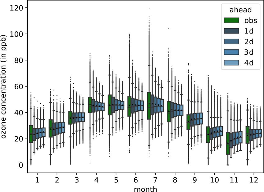
F. Kleinert et al.: IntelliO3-ts v1.0                                                                                                                               3

Table 1. Overview of the literature on ozone forecasts with neural networks. Machine learning (ML) types are abbreviated as FC for fully
connected, CNN for convolutional neural network, RNN for recurrent neural network, and LSTM for long short-term memory. We use the
following abbreviations for time periods: yr for years and m for month.

  Citation                        ML type            Total number of   Stations for      Time period                            Comments
                                                     stations          training
  Comrie (1997)                   FC                 8                 8                 5 yr                                   Random split for train, val
  Cobourn et al. (2000)           FC                 7                 7                 5 yr (train) + 1 yr (val) + 1 yr
                                                                                         (test)
  Prybutok et al. (2000)          FC                 1                                   4m + 1m
  Gardner and Dorling (2001)      FC                 6                 6                 12 yr
  Eslami et al. (2020)            CNN                25                25                3 yr train 1 yr test                   Random split
  Liu et al. (2019)               Attention RNN      2                 2                 10 m (train), 7 d (test)               Analysis for PM2.5
  Maleki et al. (2019)            FC                 4                 4                 1 yr                                   Random split for train, val, test
  Silva et al. (2019)             FC                 2                 1                 13 yr (train, val test); 14 yr (test   Dry deposition of O3 ; random
                                                                                         on second station)                     split on first station
  Abdul Aziz et al. (2019)        FC                 1                 1                 7d                                     Individual measurements for
                                                                                                                                study
  Pawlak and Jarosławski (2019)   FC                 2                 2                 6 m (train) + 6 m (test)               Individual network per station
  Seltzer et al. (2020)           FC                 3557              3557              15 yr                                  focus on trends
  Ma et al. (2020)                Bidir. LSTM        19 (standard) +   19 (standard) +   9m                                     Exploration of transfer learning
                                                     48 (transfer)     48 (transfer)
  Sayeed et al. (2020)            CNN                21                21                3 yr (train) + 1 yr (test/re-train)    Re-train model for each
                                                                                                                                prediction
  Zhang et al. (2020)             CNN LSTM           35                35                19 m                                   Gridded forecast
  This study                      Inception blocks   329               312               18 yr

   Besides the trace gas concentrations, ozone levels also                       Table 2. Input variables and applied daily statistics according to
depend on meteorological variables. Due to the scarcity                          Table 3.
of reported meteorological measurements at the air quality
monitoring sites, we extracted time series of meteorologi-                               Variable                                      Daily statistics
cal variables from the 6 km resolution COSMO reanalysis                                  NO                                            dma8eu
(Bollmeyer et al., 2015, COSMO-REA6) and treat those as                                  NO2                                           dma8eu
observations.                                                                            O3                                            dma8eu
   All data used in this study were retrieved from the                                   Cloud cover                                   average
Tropospheric Ozone Assessment Report (TOAR) database                                     Planetary boundary layer height               maximum
(Schultz et al., 2017) via the representational state transfer                           Relative humidity                             average
(REST) application programming interface (API) at https:                                 Temperature                                   maximum
                                                                                         Wind’s u component                            average
//join.fz-juelich.de (last access: 12 November 2020). The
                                                                                         Wind’s v component                            average
air quality measurements were provided by the German
Umweltbundesamt, while the meteorological data were ex-
tracted from the COSMO-REA6 reanalysis as described
above. These reanalysis data cover the period from 1995 to                       to sample all chemical quantities during the same time pe-
2015 with some gaps due to incompleteness in the TOAR                            riods and with similar averaging times. While the dma8eu
database. As discussed in the US EPA guidelines on air qual-                     metrics is calculated based on data starting at 17:00 LT on
ity forecasting (Dye, 2003), ozone concentrations typically                      the previous day, the daily mean/max values, for example,
depend on temperature, irradiation, humidity, wind speed,                        would be calculated based on data starting from the current
and wind direction. The vertical structure of the lowest por-                    day. To test the impact of using different metrics for ozone
tion of the atmosphere (i.e. the planetary boundary layer)                       precursors, we also trained the model from scratch with ei-
also plays an important role, because it determines the rate                     ther mean or maximum concentrations of NO and NO2 as
of mixing between fresh pollution and background air. Since                      inputs. The results of these runs were hardly distinguishable
irradiation data were not available from the REST interface,                     from the results presented below.
we used cloud cover together with temperature as proxy vari-                        As described above, ozone concentrations are less vari-
ables.                                                                           able at stations, which are further away from primary pol-
   Table 2 shows the list of input variables used in this study,                 lutant emission sources. We therefore selected those stations
and Table 3 describes the daily statistics that were applied                     from the German air quality monitoring network, which are
to the hourly data of each variable. The choice of using the                     labelled as “background” stations according to the European
dma8eu metrics for NO and NO2 was motivated by the idea                          Environmental Agency (EEA), Airbase classification.

https://doi.org/10.5194/gmd-14-1-2021                                                                            Geosci. Model Dev., 14, 1–25, 2021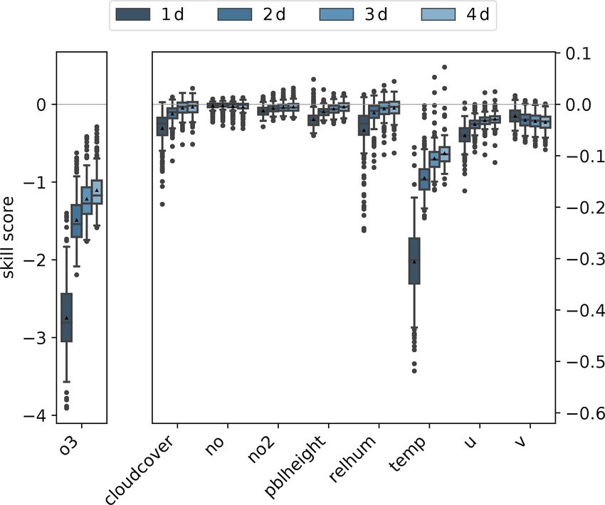
4 F. Kleinert et al.: IntelliO3-ts v1.0
Table 3. Definitions of statistical metrics in TOAR analysis relevant for this study. Adopted form Schultz et al. (2017, Supplement 1, Table 6,
therein).
Name Description
data_capture Fraction of valid (hourly) values available in the aggregation period.
average_values Daily [. . . ] average value. No data capture criterion is applied, i.e. a daily average is valid if at least one hourly
value of the day is present.
dma8eu As dma8epa but using the EU definition of the daily 8 h window starting from 17:00 LT of the previous day.
(dma8epa: daily maximum 8 h average statistics according to the US EPA definition. The 8 h averages are calculated
for 24 bins starting at 00:00 LT. The 8 h running mean for a particular hour is calculated on the concentration for
that hour plus the following 7 h. If less than 75 % of data are present (i.e. less than 6 h), the average is considered
missing. Note that in contrast to the official EPA definition, a daily value is considered valid if at least one 8 h
average is valid.)
maximum Daily maximum value. No data capture criterion is applied; i.e. a daily maximum is valid if at least one hourly value
of the day is present.
data comprise 312 stations, validation data 211 stations, and
testing 203 stations. This is by far the largest air quality time
series dataset that has been used in a machine learning study
so far (see Table 1).
Supervised learning techniques require input data (X) and
a corresponding label (y) which we create for each station of
the three sets as depicted in Algorithm 1.
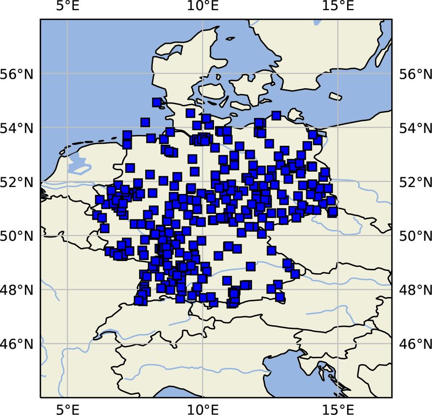
Figure 1. Map of central Europe showing the location of German
measurement sites used in this study. This figure was created with
Cartopy (Met Office, 2010–2015). Map data © OpenStreetMap con-
tributors.
2.2 Data processing Samples within the same dataset (train, validation, and
test) can overlap which means that one missing data point
We split the individual station time series into three non- would appear up to seven times in the inputs X and up to
overlapping time periods for training, validation, and testing four times in the labels y. Consequently, one missing value
which we will refer to as “set” from now on (see Fig. 2). We will cause the removal of 11 samples (algorithm 1, line 7).
only used stations which at least have 1 year of valid data in As we want to keep the number of samples as high as pos-
one set. Firstly, the time span of the training dataset is rang- sible, we decided to linearly interpolate (algorithm 1, line 2)
ing from 1 January 1997 to 31 December 2007. Secondly, the the time series if only one consecutive value is missing. Ta-
validation set is ranging from 1 January 2008 to 31 Decem- ble 4 shows the number of stations per dataset (train, val, test)
ber 2009. Thirdly, the test set ranges from 1 January 2010 to and the corresponding amount of samples (pairs of inputs X
31 December 2015. and labels y) per dataset. Moreover, Table A1 summarises all
Due to changes in the measurement network over time,
the number of stations in the three datasets differ: training
Geosci. Model Dev., 14, 1–25, 2021 https://doi.org/10.5194/gmd-14-1-2021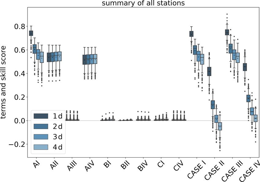
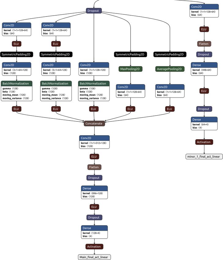
F. Kleinert et al.: IntelliO3-ts v1.0                                                                                                       5

Figure 2. Data availability diagram combined for all variables and all stations. The training set is coloured in orange, the validation set in
green, and the test set in blue. Gaps in 1999 and 2003 are caused by missing model data in the TOAR database.

samples per station individually. Figure 1 shows a map of all            sizes did not yield significantly different results. Before cre-
station locations.                                                       ating the different training batches, we permute the ordering
   We trained the neural network (details on the network                 of samples per station in the training set to ensure that the dis-
architecture are given in Sect. 3) with data of the train-               tribution of each batch is similar to those of the full training
ing set and tuned hyperparameters exclusively on the val-                dataset (algorithm 1, line 9). Otherwise, each batch would
idation dataset. For the final analysis and model evalua-                have an under-represented season and consequently would
tion, we use the independent test dataset, which was nei-                lead to undesired looping during training (e.g. no winter val-
ther used for training the models parameters, nor for tuning             ues in the first batch, no autumn values in the second batch).
the hyperparameters. Random sampling, as is often done in
other machine learning applications, and occasionally even
in other air quality or weather applications of machine learn-           3    Model setup
ing, would lead to overly optimistic results due to the multi-
day auto-correlation of air quality and meteorological time              Our machine learning model is based on a convolutional
series. Horowitz and Barakat (1979) already pointed to this              layer neural network (LeCun et al., 1998), which was initially
issue when dealing with statistical tests. Likewise, the alter-          designed for pattern recognition in computer vision applica-
native split of the dataset into spatially segregated data could         tions. It has been shown that such model architectures work
lead to the undesired effect that two or more neighbouring               equally well on time series data as other neural network ar-
stations with high correlation between several paired vari-              chitectures, which have been especially designed for this pur-
ables fall into different datasets. Again, this would result in          pose, such as recurrent neural networks or LSTMs (Dauphin
overly optimistic model results.                                         et al., 2017; Bai et al., 2018). Schmidhuber (2015) provides
   By applying a temporal split, we ensure that the training             a historical review on different deep learning methods, while
data do not directly influence the validation and test datasets.         Ismail Fawaz et al. (2019) focus especially on deep neural
Therefore, the final results reflect the true generalisation ca-         networks for time series.
pability of our forecasting model.                                          Our neural network named IntelliO3-ts, version 1.0, pri-
   In accordance with other studies, our initial deep learning           marily consists of two inception blocks (Szegedy et al.,
experiments with a subset of this data have shown that neural            2015), which combine multiple convolutions, execute them
networks, just as other classical regression techniques, have a          in parallel, and concatenate all outputs in the last layer of
tendency to focus on the mean of the distribution and perform            each block. Figure A2 depicts one inception block including
poorly on the extremes. However, especially the high concen-             the first input layer, while Figs. A2 and A3 together show the
tration events are crucial in the air quality context due to their       entire model architecture including the final flat and output
strong impact on human health and the adverse crop effects.              layers. We treat each input variable (see Table 2) as an indi-
Extreme values occur relatively seldomly in the dataset, and             vidual channel (like R, G, B in images) and use time as the
it is therefore difficult for the model to learn their associ-           first dimension (this would correspond to the width axis of an
ated patterns correctly. To increase the total number of val-            image). Inputs (X) consist of the variable values from 7 d (−6
ues on the tails of the distribution during training, we append          to 0 d). Outputs are ozone concentration forecasts (dma8eu)
all samples where the standardised label (i.e. the normalised            for lead times up to 4 d (1 to 4 d). Therefore, we change the
ozone concentration) is < −3 or > 3 for a second time on the             kernel sizes in the inception blocks from 1 × 1, 3 × 3, and
training dataset (algorithm 1, line 8).                                  5 × 5, as originally proposed by Szegedy et al. (2015), to
   We selected a batch size of 512 samples (algorithm 1,                 1 × 1, 3 × 1, and 5 × 1. This allows the network to focus on
line 10), because this size is a good compromise between                 different temporal relations. The 1 × 1 convolutions are also
minimising the loss function and optimising computing time               used for information compression (reduction of the number
per trained epoch. Experiments with larger and smaller batch             of filters) before larger convolutional kernels are applied (see

https://doi.org/10.5194/gmd-14-1-2021                                                               Geosci. Model Dev., 14, 1–25, 2021
6                                                                                                           F. Kleinert et al.: IntelliO3-ts v1.0

Table 4. Number of stations, total number of samples (pairs of X and y), and various statistics of number of samples per station in the
training, validation, and test datasets. The number of stations per set varies as not all stations have data through the full period (see Table A1
for details).

                 No. of stations   No. of samples     Mean      SD      Min       5%    10 %    25 %    50 %       75 %   90 %    95 %     Max
    Training                312           643 788      2063    802      369       668    939    1426    2191       2902   2989    3011    3045
    Validation              211           145 030       687     61      370       532    625     690     710        721    721     721     721
    Test                    203           212 093      1044     92      466       759    983    1056    1075       1086   1086    1086    1086

Szegedy et al., 2015). This decreases the computational costs                 system which is operated by the Jülich Supercomputing Cen-
for training and evaluating the network. In order to conserve                 tre (see also Sect. A4 for further details regarding the soft-
the initial input shape of the first dimension (time), we apply               ware and hardware configurations).
symmetric padding to minimise the introduction of artefacts
related to the borders.
   While the original proposed concept of inception blocks                    4     Evaluation metrics and reference models
has one max-pooling tower alongside the different convolu-
                                                                              In general, one can interpret a supervised machine learn-
tion stacks, we added a second pooling tower, which calcu-
                                                                              ing approach as an attempt to find an unknown function ϕ
lates the average on a kernel size of 3×1. Thus, one inception
                                                                              which maps an input pattern (X) to the corresponding labels
block consists of three convolutional towers and two pooling
                                                                              or the ground truth (y). The machine learning model is con-
(mean and max) towers. A tower is defined as a collection
                                                                              sequently an estimator (ϕ̂) which maps X to an estimate ŷ of
or stack of successive layers. The outputs of these towers
                                                                              the ground truth. The goodness of the estimate is quantified
are concatenated in the last layer of an inception block (see
                                                                              by an error function, which the network tries to minimise
Fig. A2). Between individual inception blocks, we added
                                                                              during training. As the network is only an estimator of the
dropout layers (Srivastava et al., 2014) with a dropout rate of
                                                                              true function, the mapping generally differs:
0.35 to improve the network’s generalisation capability and
prevent overfitting.                                                          ϕ (X) = y 6 = ŷ = ϕ̂ (X) .                                     (4)
   Moreover, we use batch normalisation layers (Ioffe and
Szegedy, 2015) between each main convolution and activa-                         To evaluate the genuine added value of any meteorological
tion layer to accelerate the training process (Fig. A2). Those                or air quality forecasting model, it is essential to apply proper
normalisations ensure that for each batch the mean activation                 statistical metrics. The following section describes the veri-
is zero with standard deviation of 1. As proposed in Szegedy                  fication tools, which are used in this study. We provide ad-
et al. (2015), the network has an additional minor tail which                 ditional information on joint distributions as introduced by
helps to eliminate the vanishing gradient problem. Addition-                  Murphy and Winkler (1987) in Sect. A2.
ally, the minor tail helps to spread the internal representation
of data as it strongly penalises large errors.                                4.1    Scores and skill scores
   The loss function for the main tail is the mean squared
                                                                              To quantify a model’s informational content, scores like the
error:
                                                                              mean squared error (Eq. 5) are defined to provide an absolute
          1X                      2
Lmain =          yi,true − yi,pred ,                         (2)              performance measure, while skill scores provide a relative
          n i                                                                 performance measure related to a reference forecast (Eq. 6).
while the loss function of the minor tail is                                                      N
                                                                                               1 X
          1X                         4                                       MSE (m, o) =           (mi − oi )2 ≥ 0                          (5)
Lminor =         |yi,true − yi,pred | .                           (3)                          N i=1
          n i
   All activation functions are exponential linear units                      Here, N is the number of forecast–observation pairs, m is a
(ELUs) (Clevert et al., 2016); only the final output activa-                  vector containing all model forecasts, and o is a vector con-
tions are linear (minor and main tail).                                       taining the observations (Murphy, 1988).
   The network is built with Keras 2.2.4 (Chollet, 2015) and                     A skill score S may be interpreted as the percentage of
uses TensorFlow 1.13.1 (Abadi et al., 2015) as the backend.                   improvement of A over the reference Aref . Its general form is
We use Adam (Kingma and Ba, 2014) as optimiser and apply                             A − Aref
an initial learning rate of 10−4 (see also Sect. A5).                         S=                 .                                            (6)
                                                                                    Aperf − Aref
   We train the model for 300 epochs on the Jülich Wizard for
European Leadership Science (JUWELS; Jülich Supercom-                         Here, A represents a general score, Aref is the reference
puting Centre, 2019) high-performance computing (HPC)                         score, and Aperf the perfect score.

Geosci. Model Dev., 14, 1–25, 2021                                                                   https://doi.org/10.5194/gmd-14-1-2021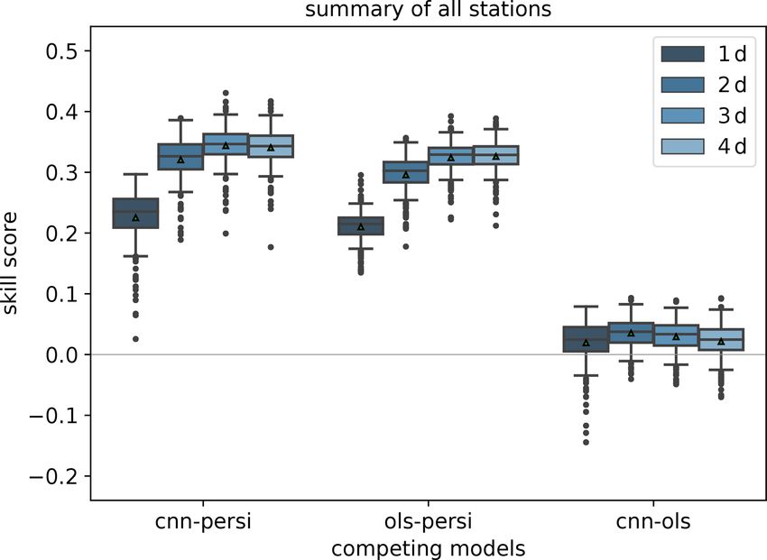
F. Kleinert et al.: IntelliO3-ts v1.0                                                                                             7

   For A = Aref , S becomes zero, indicating that the forecast      reference does not include any direct information on the test
of interest has no improvements over the reference forecast.        set. Therefore, one can access the information if the forecast
A value of S > 0 indicates an improvement over the refer-           of interest captures features which are not directly present in
ence, while S < 0 indicates a deterioration. The informative        the training and validation set.
value of a skill score strongly depends on the selected refer-         Finally, the fourth reference (Aref : r = µ∗ , Case IV) is
ence forecast. In the case of the mean squared error (Eq. 5),       an external multi-value climatology. A tabular summary ex-
the perfect score is equal to zero and Eq. (6) reduces to           plaining the individual formulae and terms following Mur-
                                                                    phy (1988) is given in Sect. A3. The last two references are
                    MSE (m, o)
S (m, r, o) = 1 −              ,                             (7)    calculated on a much longer time series than the first ones.
                    MSE (r, o)
where r is a vector containing the reference forecast.              4.2.3    OLS reference model

4.2     Reference models                                            The third reference model is an ordinary least-square (OLS)
                                                                    model. We train the OLS model by using the statsmod-
We used three different reference models: persistence, cli-         els package v0.10 (Seabold and Perktold, 2010). The OLS
matology, and an ordinary least-square model (linear regres-        model is trained on the same data as the neural network
sion). For the climatological reference, we create four sub-        (training set) and serves as a linear competitor.
reference models (see Sect. 4.2.2). In the following, we in-
troduce our basic reference models.
                                                                    5     Results
4.2.1    Persistence model
                                                                    As described in Sect. 3, we split our data into three subsets
One of the most straightforward models to build, which in           (training, validation, and test set). We only used the inde-
general has good forecast skills on short lead times, is a per-     pendent test dataset to evaluate the forecasting capabilities
sistence model. Today’s observation of ozone dma8eu con-            of the IntelliO3-ts network. During training and hyperpa-
centration is also the prediction for the next 4 d. Obviously,      rameter optimisation, only the training and validation sets
the skill of persistence decreases with increasing lead time.       were used, respectively. Therefore, the following results re-
The good performance on short lead times is mainly due to           flect the true generalisation capability of IntelliO3-ts. Before
the facts that weather conditions influencing ozone concen-         discussing the results in detail below, we would like to point
trations generally do not change rapidly, and that the chemi-       out again that this is the first time that one neural network
cal lifetime of ozone is long enough.                               has been trained to forecast data from an entire national air
                                                                    quality monitoring station network. Also, the network has
4.2.2    Climatological reference models                            been trained exclusively with time series data from air pollu-
                                                                    tant measurements and a meteorological reanalysis. No addi-
We create four different climatological reference models            tional information, such as geographic coordinates, or other
(Case I to Case IV), which are based on the climatology of          hints that could be used by the network to perform a station
observations by following Murphy (1988) (also with respect          classification task, has been used. The impact of such extra
to their terminology, which means that the reference score          information will be the subject of another study.
Aref is calculated by using the reference forecast r).
   The first reference forecast (Aref : r = o, Case I) is the in-   5.1     Forecasting results
ternal single value climatology which is the mean of all ob-
servations during the test period. This unique value is then        Figure 3 shows the observed monthly O3 –dma8eu distribu-
applied as reference for all forecasts. As this forecast has        tion (green) and the corresponding network predictions for a
only one constant value which is the expectation value, this        lead time of up to 4 d (dark to light blue) summarised for all
reference model is well calibrated but not refined at all.          203 stations in the test set. The network clearly captures the
   The second reference (Aref : r = o∗ , Case II) is an inter-      seasonal cycle. Nonetheless, the arithmetic mean (black tri-
nal multi-value climatology. Here, we calculate 12 arithmetic       angles) and the median tend to shift towards their respective
means, where each of the means is the monthly mean over             annual mean with increasing lead time (see also Fig. 6). In
all years in the test set (one mean for all Januaries from          spring and autumn, the observed and forecasted distributions
2012 to 2015, one for all Februaries, etc.). The corresponding      match well, while in summer and wintertime the network un-
monthly mean is applied as reference. Therefore, Case II al-        derestimates the interquartile range (IQR) and does not re-
lows testing if the model has skill in reproducing the seasonal     produce the extremes values (for example, the maxima in
cycle of the observations.                                          July/August or the minima in December/January/February).
   The third reference (Aref : r = µ, Case III) is an external
single value climatology which is the mean of all available
observations during the training and validation periods. This

https://doi.org/10.5194/gmd-14-1-2021                                                        Geosci. Model Dev., 14, 1–25, 2021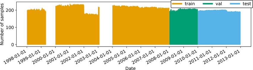
8                                                                                                 F. Kleinert et al.: IntelliO3-ts v1.0

Figure 3. Monthly dma8eu ozone concentrations for all test stations   Figure 4. Skill scores of the IntelliO3-ts (cnn) versus the two ref-
as boxplots. Measurements are denoted by “obs” (green), while the     erence models’ persistence (persi) and ordinary least square (ols)
forecasts are denoted by “1 d” (dark blue) to “4 d” (light blue).     based on the mean squared error; separated for all lead times (1 d
Whiskers have a maximal length of one interquartile range. The        (dark blue) to 4 d (light blue)). Positive values denote that the
black triangles denote the arithmetic means.                          first mentioned prediction model performs better than the reference
                                                                      model (mentioned as second). The triangles denote the arithmetic
                                                                      means.
5.2   Comparison with competitive models

The skill scores based on the mean squared error (MSE)
evaluated over all stations in the test set are summarised in
Fig. 4. In the left and centre groups of boxes and whiskers,
the IntelliO3-ts model (labelled “CNN”) and the OLS model
are compared against persistence as reference. The right
group of boxes and whiskers shows the comparison between
IntelliO3-ts and OLS. The mean skill score for IntelliO3-ts
against persistence is positive and increases with time. The
OLS forecast shows similar behaviour in terms of its tempo-
ral evolution but exhibits a slightly lower skill score through-
out the 4 d forecasting period. The increases in skill score in
both cases is mainly due to the decreasing performance of
the persistence model (see also Sect. 4.2.1). Consequently,
IntelliO3-ts shows a positive skill score when the OLS model
is used as a reference, indicating a small genuine added value
over the OLS model.                                                   Figure 5. Skill scores of IntelliO3-ts with respect to climatological
   In comparison with climatological reference forecasts as           reference forecasts: with internal single value reference (Case I),
introduced in Sect. 4.1 and summarised in Table A2, the skill         internal multi-value (monthly) reference (Case II), external single
scores are high for the first lead time (1 d) and decrease with       (Case III), and external multi-value (monthly) reference (Case IV)
                                                                      for all lead times from 1 d (dark blue) to 4 d (light blue). Triangles
increasing lead time (Fig. 5). Both cases with a single value
                                                                      denote the arithmetic means.
as reference (internal Case I, external Case III) maintain a
skill score above 0.4 over the 4 d. These high skill scores are a
direct result of the fact that IntelliO3-ts captures the seasonal
cycle as shown in Fig. 3, while the reference forecasts only          test set itself. These results show that, for the vast majority
report the overall mean as a single value prediction.                 of stations, our model performs much better than a seasonal
   If the reference includes the seasonal variation (Case II          climatology for a 1 d forecast, and it is still substantially bet-
and Case IV), the IntelliO3-ts skill score is still better than       ter than the climatology after 2 d. However, there are some
0.4 for the first day (1 d), but then it decreases rapidly and        stations which yield a negative skill score even on day 2
even becomes negative on day 4 for Case II. The skill scores          in the Case II comparison. Longer-term forecasts with this
for Case II are lower than for Case IV as the reference cli-          model setup do not add value compared to the computation-
matology (i.e. the monthly mean values) is calculated on the          ally much cheaper monthly mean climatological forecast.

Geosci. Model Dev., 14, 1–25, 2021                                                          https://doi.org/10.5194/gmd-14-1-2021
F. Kleinert et al.: IntelliO3-ts v1.0 9
5.3 Analysis of joint distributions right tail of SON is much more pronounced than for DJF,
with higher values occurring primarily in September. In the
The full joint distribution in terms of calibration refinement summer season (JJA, Fig. A6a–d), the most frequently pre-
factorisation (Sect. A2) is shown in Fig. 6a (first lead time; dicted values correspond to the location of the right mode
1 d) to d (last lead time; 4 d). The marginal distribution (re- of Fig. 6a–d. During DJF, MAM, and JJA, the model has a
finement) is shown as histogram (light grey; sample size), stronger tendency of under-forecasting with increasing lead
while the conditional distribution (calibration) is presented time (median line moves above the reference line).
by specific percentiles in different line styles. If the median
(0.5th quantile, solid line) is below the reference, the net- 5.4 Relevance of input variables
work exhibits a high bias with respect to the observations,
and vice versa. Obviously, quantiles in value regions with To analyse the impact of individual input variables on the
many data samples are more robust and therefore more credi- forecast results, we apply a bootstrapping technique as fol-
ble than quantiles in data-sparse concentration regimes (Mur- lows: we take the original input of one station, keep eight
phy et al., 1989). On the first lead time (d1; Fig. 6), the of the nine variables unaltered, and randomly draw (with re-
IntelliO3-ts network has a tendency to slightly overpredict placement) the missing variable (20 times per variable per
concentrations /30 ppb. On the other hand, the forecast un- station). This destroys the temporal structure of this specific
derestimates concentrations above '70 ppb. variable so that the network will no longer be able to use
Both very high and very low forecasts are rare (note the this information for forecasting. Compared to alternative ap-
logarithmic axis for the sample size). Therefore, the results proaches, such as re-training the model with fewer input vari-
in these regimes have to be treated with caution. Further de- ables, setting all variable values to zero, etc., this method has
tail is provided in Fig. A1, where the conditional biases are two main advantages: (i) the model does not need to be re-
shown (terms BI, BII, and BIV in Sect. A3) which decrease trained, and thus the evaluation occurs with the exact same
the maximal climatological potential skill score (term AI; see weights that were learned from the full dataset, and (ii) the
also Table A2). distribution of the input variable remains unchanged so that
With increasing lead time, the model looses its capability adverse effects, for example, due to correlated input vari-
to predict concentrations close to zero and high concentra- ables, are excluded. However, we note that this method may
tions above 80 ppb. The marginal distribution develops a pro- underestimate the impact of a specific variable in the case of
nounced bimodal shape which is directly linked to the con- correlated input data, because in such cases the network will
ditional biases. The number of high (extreme) ozone concen- focus on the dominant feature (here ozone). Also, this analy-
trations is relatively low, resulting in few training examples. ses only evaluates the behaviour of the deep learning model
The network tries to optimise the loss function with respect to and does not evaluate the impact of these variables on actual
the most common values. As a result, predictions of concen- ozone formation in the atmosphere.
trations near the mean value of the distribution are generally After the randomisation of one variable, we apply the
more correct than predictions of values from the fringes of trained model on this modified input data and compare the
the distribution. Moreover, this also explains why the model new prediction with the original one. For comparison, we ap-
does not perform substantially better than the monthly mean ply the skill score (Eq. 6) based on the MSE where we use
climatology forecasts (Case II, Case IV). This problem also the original forecast as a reference. Consequently, the skill
becomes apparent in other studies. For example, Sayeed et al. score will be negative if the bootstrapped variable has a sig-
(2020) focus their categorical analysis on a threshold value nificant impact on model performance. Figure 7 shows the
of 55 ppbv (maximum 8 h average) which corresponds to the skill scores for all variables (x axis) and lead times (dark (1 d)
air quality index value “moderate” (AQI 51 to 100), instead to light blue (4 d) boxplots). Ozone is the most crucial input
of the legal threshold value of 70 ppbv (U.S. Environmen- variable, as it has by far the lowest skill score for all lead
tal Protection Agency, 2016, Table 5, therein), as the model times. With increasing lead time, the skill score increases but
shows better skills in this regime. stays lower than for any other variable. In contrast, the model
To shed more light on the factors influencing the forecast does not derive much skill from the variables nitrogen oxide,
quality, we analyse the network performance individually nitrogen dioxide, and the planetary boundary layer height. In
for each season (DJF, MAM, JJA, and SON). Conditional other words, the network does not perform worse, when ran-
quantile plots for individual seasons can be found in the Ap- domly drawn values replace one of those original time series.
pendix (Sect. A6). As mentioned above, the bimodal shape of Relative humidity, temperature, and the wind’s u component
the marginal distribution is mainly caused by the network’s have an impact on the model performance. With increasing
weakness to predict very high and low ozone concentrations. lead time, these influences decrease.
Moreover, the seasonal decomposition shows that the left
mode is caused by the fall (SON) and winter (DJF) seasons
(Figs. A7a–d and A4a–d). In both seasons, the most com-
mon values fall into the same concentration range, while the
https://doi.org/10.5194/gmd-14-1-2021 Geosci. Model Dev., 14, 1–25, 202110 F. Kleinert et al.: IntelliO3-ts v1.0
Figure 6. Conditional quantile plot for all IntelliO3-ts predictions for a lead time of 1 d (a), 2 d (b),
3 d (c), and 4 d (d). Conditional percentiles
(0.10th and 0.90th, 0.25th and 0.75th and 0.50th) from the conditional distribution f oj |mi are shown as lines in different styles. The
reference line indicates a hypothetical perfect forecast. The marginal distribution of the forecast f (mi ) is shown as log histogram (right axis,
light grey). All calculations are done by using a bin size of 1 ppb. Quantiles are smoothed by using a rolling mean of a window size of 3.
(After Murphy et al., 1989.)
6 Limitations and additional remarks shall be transformed into an operational system, we suggest
applying online learning and use the latest available data for
Even though IntelliO3-ts v1.0 generalises well on an unseen subsequent training cycles (see, for example, Sayeed et al.,
testing set (see Sect. 5), it still has some limitations related to 2020).
the applied data split.
By splitting the data into three consecutive, non-
overlapping sets, we ensure that the datasets are as inde-
pendent as possible. On the other hand, this independence 7 Conclusions
comes at the cost that changes of trends in the input variables
may not be captured, especially as our input data are not de- In this study, we developed and evaluated IntelliO3-ts, a deep
trended. Indeed, at European non-urban measurement sites, learning forecasting model for daily near-surface ozone con-
several ozone metrics related to high concentrations (e.g. centrations (dma8eu) at arbitrary air quality monitoring sta-
fourth highest daily maximum 8 h (4MDA8) or the 95th per- tions in Germany. The model uses chemical (O3 , NO, NO2 )
centile of hourly concentrations) show a significant decrease and meteorological time series of the previous 6 d to create
during our study period (1997 to 2015) (Fleming et al., 2018; forecasts for up to 4 d into the future. IntelliO3-ts is based
Yan et al., 2018). Our data-splitting method for evaluating on convolutional inception blocks, which allow us to cal-
the generalisation capability is conservative in the sense that culate concurrent convolutions with different kernel sizes.
we evaluate the model on the test set, which has the largest The model has been trained on 10 years of data from 312
possible distance to the training set. If our research model background stations in Germany. Hyperparameter tuning and
Geosci. Model Dev., 14, 1–25, 2021 https://doi.org/10.5194/gmd-14-1-2021F. Kleinert et al.: IntelliO3-ts v1.0 11
only have a small effect on the model performance, while the
time series of NO, NO2 , and planetary boundary layer (PBL)
have no impact.
The IntelliO3-ts network extends previous work by using a
new network architecture, and training one model on a much
larger set of measurement station data and longer time peri-
ods. In light of Rasp and Lerch (2018), who used several neu-
ral networks to postprocess ensemble weather forecasts, we
applied meteorological evaluation metrics to perform a point-
by-point comparison, which is not common in the field of
deep learning. We hope that the forecast quality of IntelliO3-
ts can be further improved if we take spatial context informa-
tion into account so that the advection of background ozone
and ozone precursors can be learned by the model.
Figure 7. Skill scores of bootstrapped model predictions having the
original forecast as the reference model are shown as boxplots for
all lead times from 1 d (dark blue) to 4 d (light blue). The skill score
for ozone is shown on the left y axis, while the skill score of the
other variables is shown on the right y axis.
model evaluation were done with independent datasets of 2
and 6 years length, respectively.
The model generalises well and generates good quality
forecasts for lead times up to 2 d. These forecasts are su-
perior compared to the reference persistence, ordinary least
squares, annual, and seasonal climatology models. After 2 d,
the forecast quality degrades, and the forecast adds no value
compared to a monthly mean climatology of dma8eu ozone
levels. We could primarily attribute this to the network’s ten-
dency to converge to the mean monthly value. The model
does not have any spatial context information which could
counteract this tendency. Near-surface ozone concentrations
at background stations are highly influenced by air mass ad-
vection, but the IntelliO3-ts network has no way of taking up-
wind information into account yet. We will investigate spatial
context approaches in a forthcoming study.
We observed that the model loses refinement with increas-
ing lead time which results in unsatisfactory predictions on
the tails of the observed ozone concentration. We were able
to attribute this weakness to the under-representation of ex-
treme (either very small or high) levels in the training dataset.
This is a general problem for machine learning applications
and regression methods. The machine learning community is
investigating possible solutions to lessen the impact of such
data imbalances, but their adaptation is beyond the scope of
this paper as proposed techniques are not directly applicable
to those time series (auto-correlation time).
Bootstrapping individual time series of the input data to
analyse the importance of those variables on the predictive
skill showed that the model mainly focused on the previ-
ous ozone concentrations. Temperature and relative humidity
https://doi.org/10.5194/gmd-14-1-2021 Geosci. Model Dev., 14, 1–25, 202112 F. Kleinert et al.: IntelliO3-ts v1.0
Appendix A Table A1. Continued.
A1 Information on used stations Training Val Test
Stat. ID
Table A1 lists all measurement stations which we used in this
study. The table also shows the number of samples (X, y) for DEBW021 1579 – –
each of the three datasets (training, validation, and test). DEBW023 1430 721 1078
DEBW024 3011 713 1086
DEBW025 1530 – –
Table A1. Number of samples (input and output pairs) per station
DEBW026 3005 721 –
separated by training, validation (val), and test dataset. “–” denotes
DEBW027 3005 699 1075
no samples in a set.
DEBW028 1510 – –
DEBW029 3012 721 1086
Training Val Test DEBW030 2966 – –
Stat. ID DEBW031 2970 711 1069
DEBW032 2648 – –
DEBB001 1104 – – DEBW034 3045 707 –
DEBB006 1455 – – DEBW035 2281 – –
DEBB007 – 721 1086 DEBW036 1183 – –
DEBB009 1438 – – DEBW037 3023 721 –
DEBB021 2512 705 1052 DEBW039 2999 710 1086
DEBB024 2592 – – DEBW041 1581 – –
DEBB028 1353 – – DEBW042 2617 708 1067
DEBB031 2577 – – DEBW044 1571 – –
DEBB036 1008 – – DEBW045 656 – –
DEBB038 1245 – – DEBW046 2990 699 1086
DEBB040 760 – – DEBW047 1563 – –
DEBB042 2902 721 1086 DEBW049 646 – –
DEBB043 2194 – – DEBW050 1556 – –
DEBB048 2473 721 1075 DEBW052 2652 721 1078
DEBB050 2510 721 – DEBW053 1574 – –
DEBB051 1006 – – DEBW054 1566 – –
DEBB053 2115 706 1086 DEBW056 2938 721 1086
DEBB055 1887 721 1053 DEBW057 644 – –
DEBB063 1392 721 1086 DEBW059 2974 721 1086
DEBB064 1480 721 1086 DEBW060 1571 – –
DEBB065 1411 699 1086 DEBW065 1540 – –
DEBB066 1451 721 1086 DEBW072 480 – –
DEBB067 1073 721 1086 DEBW076 3035 721 708
DEBB075 – 721 1079 DEBW081 2654 721 1079
DEBB082 – 622 1086 DEBW084 1444 721 1042
DEBB083 – – 1086 DEBW087 3043 713 1086
DEBE010 1372 707 1035 DEBW094 2188 – –
DEBE032 2441 690 1060 DEBW102 1122 – –
DEBE034 2506 671 1031 DEBW103 2525 721 –
DEBE051 2433 694 1053 DEBW107 1801 714 1086
DEBE056 2481 678 1055 DEBW110 1107 721 –
DEBE062 1941 677 1069 DEBW111 1083 703 –
DEBW004 1440 721 1086 DEBW112 651 721 1079
DEBW006 1451 721 1086 DEBW113 678 – –
DEBW007 1440 699 – DEBY002 2924 721 747
DEBW008 656 – – DEBY004 2917 707 1028
DEBW010 3041 708 1086 DEBY005 2959 714 1086
DEBW013 1432 710 1079 DEBY013 1412 652 980
DEBW019 2962 710 1078 DEBY017 1250 – –
DEBW020 1520 – –
Geosci. Model Dev., 14, 1–25, 2021 https://doi.org/10.5194/gmd-14-1-2021F. Kleinert et al.: IntelliO3-ts v1.0 13
Table A1. Continued.
Training Val Test Table A1. Continued.
Stat. ID Training Val Test
DEBY020 2976 721 1013 Stat. ID
DEBY031 2927 678 1072
DEBY032 2975 721 711 DEHE048 1043 – –
DEBY034 1555 – – DEHE050 1014 – –
DEBY039 2554 721 1067 DEHE051 2331 721 1086
DEBY047 1895 721 754 DEHE052 2078 713 1086
DEBY049 2918 693 1066 DEHE058 789 721 1086
DEBY052 2929 708 1035 DEHE060 704 672 1086
DEBY062 1411 704 748 DEHH008 1439 721 1086
DEBY072 2907 690 1055 DEHH021 2624 710 1086
DEBY077 1409 721 724 DEHH033 2148 682 1067
DEBY079 2878 721 671 DEHH047 2175 696 1086
DEBY081 2932 523 713 DEHH049 2150 721 1075
DEBY082 1592 – – DEHH050 2131 721 1069
DEBY088 2986 713 1062 DEMV001 794 – –
DEBY089 2644 721 1086 DEMV004 2908 721 1058
DEBY092 616 – – DEMV007 2986 721 1053
DEBY099 1828 703 725 DEMV012 2885 710 1086
DEBY109 1310 713 1071 DEMV017 2507 708 1086
DEBY113 1347 706 1086 DEMV018 2113 710 –
DEBY118 937 705 727 DEMV019 1429 706 1086
DEBY122 – – 877 DEMV021 600 688 1072
DEHB001 2567 710 953 DEMV024 – – 908
DEHB002 2287 702 1053 DENI011 2611 452 1086
DEHB003 2546 695 – DENI016 3034 627 1051
DEHB004 1428 708 1037 DENI019 2919 – –
DEHB005 2518 683 1066 DENI020 2984 667 1086
DEHE001 1451 721 1086 DENI028 2927 516 1086
DEHE008 2447 707 1075 DENI029 2903 692 1086
DEHE010 1600 – – DENI031 1410 451 1079
DEHE013 – 721 1086 DENI038 2599 573 1083
DEHE017 1562 – – DENI041 2935 525 1086
DEHE018 3016 721 1086 DENI042 2939 553 1072
DEHE019 1958 – – DENI043 2941 606 1086
DEHE022 2643 721 1086 DENI051 2976 – 1072
DEHE023 2966 708 466 DENI052 2910 529 1086
DEHE024 2935 710 1086 DENI054 2997 596 1086
DEHE025 1554 – – DENI058 2398 – 1086
DEHE026 2877 697 1086 DENI059 2408 451 1079
DEHE027 1536 – – DENI060 2386 677 1086
DEHE028 2946 710 1068 DENI062 2482 625 1080
DEHE030 3028 721 1086 DENI063 2385 460 1073
DEHE032 2926 714 1075 DENI077 – – 1079
DEHE033 1835 – – DENW004 1148 – –
DEHE034 1880 – – DENW006 1367 694 1026
DEHE039 – – 812 DENW008 2511 701 1064
DEHE042 2966 721 1079 DENW010 1397 – –
DEHE043 3004 721 1074 DENW013 1830 – –
DEHE044 2543 721 1086 DENW015 1451 – –
DEHE045 2535 699 1086 DENW018 1196 – –
DEHE046 2513 714 1086 DENW028 1655 – –
DENW029 2530 – –
DENW030 2785 630 998
https://doi.org/10.5194/gmd-14-1-2021 Geosci. Model Dev., 14, 1–25, 202114 F. Kleinert et al.: IntelliO3-ts v1.0
Table A1. Continued.
Table A1. Continued.
Training Val Test
Training Val Test
Stat. ID
Stat. ID
DESL017 2785 714 1086
DENW036 1314 – –
DESL018 1656 710 1086
DENW038 2598 652 1079
DESL019 1371 472 1057
DENW042 1185 – –
DESN001 2925 689 1072
DENW047 1350 – –
DESN004 3011 705 1086
DENW050 2488 – –
DESN005 1166 – –
DENW051 1206 – –
DESN011 2613 694 1073
DENW053 1795 678 1051
DESN012 2995 721 –
DENW059 1777 648 980
DESN014 2256 – –
DENW062 1078 – –
DESN017 3028 704 –
DENW063 2816 – –
DESN019 2934 721 –
DENW064 2887 589 1052
DESN024 3017 721 –
DENW065 2877 550 1045
DESN028 401 – –
DENW066 2865 – –
DESN036 810 – –
DENW067 2473 686 1079
DESN045 2913 721 1064
DENW068 2892 447 1009
DESN050 2939 710 –
DENW071 1827 713 1071
DESN051 1451 685 1075
DENW078 1382 681 1078
DESN057 1535 – –
DENW079 2040 706 1086
DESN059 2533 714 1078
DENW080 2147 689 1043
DESN074 2534 702 1062
DENW081 2422 646 1058
DESN076 2489 717 1075
DENW094 1980 627 1058
DESN079 – – 1071
DENW095 1981 681 1071
DESN085 713 – –
DENW096 700 – –
DESN092 – 536 1057
DENW179 766 699 1079
DEST002 3020 721 1075
DENW247 – 572 1066
DEST005 802 – –
DERP001 1421 721 1068
DEST011 2924 713 1075
DERP007 2652 721 1077
DEST014 996 – –
DERP013 2883 708 1067
DEST022 805 – –
DERP014 2967 703 1061
DEST025 480 – –
DERP015 2810 710 1047
DEST028 2694 – –
DERP016 2962 721 1086
DEST030 2282 – –
DERP017 2955 721 1055
DEST031 796 – –
DERP019 1413 708 1041
DEST032 447 – –
DERP021 2996 713 1025
DEST039 2971 676 1069
DERP022 2989 701 1059
DEST044 2923 709 1086
DERP025 2918 691 1086
DEST050 2672 706 1075
DERP028 2802 678 1026
DEST052 1484 – –
DESH005 962 – –
DEST061 814 – –
DESH006 614 – –
DEST063 1241 – –
DESH008 3031 721 1053
DEST066 2991 659 1086
DESH016 2635 698 –
DEST069 2589 707 –
DESH021 1107 – –
DEST070 1488 – –
DESH023 1700 721 1066
DEST071 462 – –
DESH033 – 721 1072
DEST072 2641 703 –
DESL003 1393 713 1086
DEST077 1611 663 1086
DESL008 1371 – –
DEST078 3042 709 –
DESL011 2776 710 1086
DEST089 2467 710 1048
DESL012 – – 1086
DEST098 1422 649 1086
Geosci. Model Dev., 14, 1–25, 2021 https://doi.org/10.5194/gmd-14-1-2021F. Kleinert et al.: IntelliO3-ts v1.0 15
A2 Joint distributions
Forecasts and observations are treated as random variables.
Let p(m, o) represent the joint distribution of a model’s fore-
cast m and an observation o, which contains information on
the forecast, the observation, and the relationship between
Table A1. Continued. both of them (Murphy and Winkler, 1987). To access specific
pieces of information, we factorise the joint distribution into
Training Val Test
a conditional and a marginal distribution in two ways. The
Stat. ID first factorisation is called calibration refinement and reads
DEST104 – – 1061
DETH005 3030 721 1075 p(m, o) = p (o|m) p(m), (A1)
DETH009 2995 721 1086
DETH013 2945 710 1086 where p (o|m) is the conditional distribution of observing
DETH016 1937 – – o given the forecast m, and p(m) is the marginal distribu-
DETH018 3027 721 1086 tion which indicates how often different forecast values are
DETH020 3002 721 1086 used (Murphy and Winkler, 1987; Wilks, 2006). A continu-
DETH024 1193 – – ous forecast is perfectly calibrated if
DETH025 2542 370 –
DETH026 1474 721 1072
E (o|m) = m (A2)
DETH027 1444 705 1086
DETH036 2996 721 1086
DETH040 2926 721 1078 holds, where E (o|m) is the expected value of o given the
DETH041 3003 710 1043 forecast m. The marginal distribution p(m) is a measure of
DETH042 2993 697 1086 how often different forecasts are made and is therefore also
DETH060 2519 721 1086 called refinement or sharpness. Both distributions are impor-
DETH061 2465 721 1063 tant to evaluate a model’s performance. Murphy and Win-
DETH095 – – 1059 kler (1987) pointed out that a perfectly calibrated forecast is
DETH096 – – 898 worth nothing if it lacks refinement.
DEUB001 1202 721 1075 The second factorisation is called the likelihood-base rate
DEUB003 1436 – –
and consequently is given by
DEUB004 2746 721 932
DEUB005 1422 721 974
DEUB013 414 – – p(m, o) = p (m|o) p(o), (A3)
DEUB021 369 – –
DEUB026 1768 – – where p (m|o) is the conditional distribution of forecast m
DEUB028 2602 603 1086 given that o was observed. p(o) is the marginal distribution
DEUB029 2834 721 1062 which only contains information about the underlying rate of
DEUB030 2893 710 947 occurrence of observed values and is therefore also called the
DEUB031 1845 – – sample climatological distribution (Wilks, 2006).
DEUB032 1629 – –
DEUB033 2034 – –
A3 Mean squared error decomposition (Murphy, 1988)
DEUB034 1434 – –
DEUB035 1977 – –
This section provides additional information about the MSE
DEUB036 411 – –
DEUB038 1628 – – decomposition introduced by Murphy (1988). The MSE de-
DEUB039 1676 – – composition is performed as
DEUB040 1549 – –
n
DEUB041 781 – – 1X
MSE (m, o)= ((mi − m) − (oi − o) + (m − o))2 (A4)
DEUB042 687 – – n i=1
Total stations 312 211 203
Total samples 643 788 145 030 212 093 = (m − o)2 + σm2 + σo2 − 2σmo (A5)
2
= (m − o) + σm2 + σo2 − 2σm σo ρmo . (A6)
Here, σm (σo ) is the sample variance of the forecasts
(observations) and σmo is the sample covariance of the
forecasts and observations, which is given by σmo =
1 Pn
n i=1 (m i − m) (oi − o). ρmo is the sample coefficient of
https://doi.org/10.5194/gmd-14-1-2021 Geosci. Model Dev., 14, 1–25, 2021You can also read