Hydrological signals in tilt and gravity residuals at Conrad Observatory (Austria) - Copernicus.org
←
→
Page content transcription
If your browser does not render page correctly, please read the page content below
Hydrol. Earth Syst. Sci., 25, 217–236, 2021
https://doi.org/10.5194/hess-25-217-2021
© Author(s) 2021. This work is distributed under
the Creative Commons Attribution 4.0 License.

Hydrological signals in tilt and gravity residuals
at Conrad Observatory (Austria)
Bruno Meurers1 , Gábor Papp2 , Hannu Ruotsalainen3 , Judit Benedek2 , and Roman Leonhardt4
1 Department  of Meteorology and Geophysics, University of Vienna, 1090 Vienna, Austria
2 Geodetic and Geophysical Institute, Research Centre for Astronomy and Earth Sciences,
Loránd Eötvös Research Network, 9400 Sopron, Hungary
3 Finnish Geospatial Research Institute (FGI), National Land Survey of Finland, 02430 Masala, Finland
4 Zentralanstalt für Meteorologie und Geodynamik (ZAMG), 1190 Vienna, Austria

Correspondence: Bruno Meurers (bruno.meurers@univie.ac.at)

Received: 23 June 2020 – Discussion started: 7 July 2020
Revised: 5 November 2020 – Accepted: 23 November 2020 – Published: 14 January 2021

Abstract. The superconducting gravimeter (SG) GWR C025            1    Introduction
has monitored the time variation in gravity at the Conrad Ob-
servatory (Austria) since autumn 2007. Two tiltmeters have        The gravity field of the Earth changes temporally – mainly
operated continuously since spring 2016, namely a 5.5 m           because of external forcing but also due to the direct grav-
long interferometric water level tiltmeter and a Lippmann-        itational (Newtonian) and indirect effects of mass transport
type 2D pendulum tilt sensor. The co-located and co-oriented      in the entire Earth system. This happens at all spatial and
set up enables a wide range of investigations because the tilts   temporal scales, from local to global and from very short
are sensitive to both geometrical solid Earth deformations        term to secular. Mass transport not only changes the den-
and to gravity potential changes. The tide-free residuals of      sity distribution, which directly affects the gravity poten-
the SG and both tiltmeters clearly reflect the gravity and/or     tial, but mostly causes deformation processes due to load-
deformation effects associated with short- and long-term en-      ing (e.g. Farrell, 1972; Hinderer and Legros, 1989). Today,
vironmental processes and reveal a complex water transport        superconducting gravimeters (SGs) are the most sensitive in-
process at the observatory site. Water accumulation on the        struments for monitoring the temporal variation in the mag-
terrain surface causes short-term (a few hours) effects which     nitude of the gravity vector. The SG sensor axis is aligned
are clearly imaged by the SG gravity and N–S tilt residuals.      with a plumb line of the gravity field by a tilt compensation
Long-term (> a few days/weeks) tilt and gravity variations        system that keeps any misalignment to less than 1 µrad (Hin-
occur frequently after long-lasting rain, heavy rain or rapid     derer et al., 2007). SGs provide highly precise time series of
snowmelt. Gravity and tilt residuals are associated with the      gravity variations reflecting various geodynamical phenom-
same hydrological process but have different physical causes.     ena like Earth tides, Earth rotation, normal modes, volcanoes
SG gravity residuals reveal the gravitational effect of wa-       and environmental (including hydrological) gravity effects
ter mass transport, while modelling results exclude a purely      (e.g. Hinderer et al., 2007). Tilt sensors are sensitive to the
gravitational source of the observed tilts. Tilt residuals show   horizontal component of the gravity vector, and to rotation
the response on surface loading instead. Tilts can be strongly    of the tiltmeter base, and monitor the angle between the sen-
affected by strain–tilt coupling (cavity effect). N–S tilt sig-   sor axis and the plumb line. Both gravimeters and tiltmeters
nals are much stronger than those of the E–W component,           react on purely gravitational effects caused by the following:
which is most probably due to the cavity effect of the 144 m          – the Earth’s interaction with the Sun and planetary bodies
long tunnel being oriented in an E–W direction.                         (tides);
                                                                      – any kind of mass redistribution within the entire Earth
                                                                        system;

Published by Copernicus Publications on behalf of the European Geosciences Union.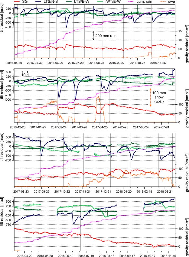
218                  B. Meurers et al.: Hydrological signals in tilt and gravity residuals at Conrad Observatory (Austria)

  – Earth rotation changes.                                         (e.g. Van Camp et al., 2017). Time-lapse microgravity sur-
                                                                    veys and SG time series provide useful estimates of wa-
Global geodynamic processes like Earth and ocean tides, nor-        ter storage changes (e.g. Van Camp et al., 2006; Davis et
mal modes and Earth rotation changes produce global defor-          al., 2008; Krause et al., 2009; Longuevergne et al., 2009;
mation of the Earth, while mass movement in the Earth sys-          Creutzfeldt et al., 2010; Lampitelli and Francis, 2010; Hec-
tem (atmosphere, hydrosphere, cryosphere and geosphere)             tor et al., 2015; Güntner et al., 2017). These techniques have
produces global to local deformation due to surface or inter-       also been successfully applied in karst environments (e.g. Ja-
nal mass loading (atmospheric pressure, hydrological water          cob et al., 2009; Fores et al., 2014; Champollion et al., 2018;
transport, magma intrusion, etc.). The sensitivity of gravime-      Mouyen et al., 2019; Watlet et al., 2020).
ters and tiltmeters, with respect to deformation effects, is           In contrast, tiltmeter signals predominantly reflect the re-
different. Radial displacement due to deformation results in        sponse on crustal deformation. Tiltmeter observations have
additional gravity changes because the sensor moves within          widely been used for hydrogeological studies. Herbst (1979)
the Earth’s gravity field. However, as displacement by local        reports tilt signals in the period range of several days ob-
load mass is very small, this effect is negligible at a local       tained from Askania borehole tiltmeter measurements in
scale (e.g. Llubes et al., 2004), except when inertial accel-       Zellerfeld–Mühlenhöhe (Germany) which occurred during
eration dominates – particularly at higher frequencies (Zürn,       precipitation events or during snowmelt periods. He ex-
2002). In contrast, tiltmeters are extremely sensitive to even      plained the tilt response by lateral fluctuations in the fracture
very small deformations. They are able to resolve tilts as          water level inducing pressure differences in adjacent fracture
small as 1 nrad, which corresponds to a vertical displace-          systems, which consequently cause the elastic bending of
ment of 1 mm over a 1000 km baseline. Figure 1 illustrates          rock structures. Jacob et al. (2010) studied water storage dy-
how tilts originate, depending on the material properties of        namics in the karst area of the Larzac plateau (France). Finite
the Earth. Gravitational (Newtonian) tilt is the change of the      element modelling suggests that deformation due to water
plumb line direction at the sensor location as it would happen      pressure changes in fractures is the most reasonable mecha-
on a non-deformable planet due to the spatial displacement          nism for explaining observed tilts after heavy precipitation.
of the equipotential surfaces. The latter is caused either by       Tenze et al. (2012) investigated the effect of underground
external forcing fields (tides) or by mass redistribution. De-      karstic water flow on tilt that was observed by two horizontal
formation produces tilt if the orientation of the surface the       pendulums in the Grotta Gigante (Italy) and revealed a linear
tilt sensor is mounted on changes with respect to the plumb         relation between the maximum tilt and the amount of wa-
line. On a non-rigid planet, both effects interfere. Deforma-       ter entering the karst system during flood events. Lesparre
tion is caused by a global stress field (as in case of the body     et al. (2017) interpreted tiltmeter observations inside the
tides) or by loading (atmosphere, water/snow accumulation           Fontaine de Vaucluse karst system as the infiltration effect of
on the surface or below, pore pressure changes, etc.). In ad-       water after rainfall, which changes the pressure in fractures
dition, as described by Harrison (1976) or Baker (1980), tilt-      and consequently induces deformation.
meter records can be strongly affected by strain–tilt coupling         Active pumping or injection experiments at different spa-
(also called strain-induced tilt) arising from deformation of       tial scales have proven the high sensitivity of tilt to pore pres-
the cavity in case of underground installations (cavity effect;     sure changes (Weise, 1992; Kümpel et al., 1996; Weise et
Baker and Lennon, 1973; King and Bilham, 1973; Agnew,               al., 1999; Fujimori et al., 2001; Jahr et al., 2008; Jahr, 2018).
1986), surface topography (topographic effect; e.g. Harrison,       Within the framework of the large-scale injection experiment
1978) and geological inhomogeneities in the close vicinity          at the German Continental Deep Drilling Program (KTB)
(geological effect; e.g. Kohl and Levine, 1995). These local        deep drilling site, Jahr et al. (2006a, b; 2008) studied the sur-
effects depend on geometry and size of the cavity in which          face deformation due to fluid-induced stress changes by bore-
the tiltmeters are installed and on the topography shape. In        hole tiltmeter array observations. They detected tilt signals
case of a horizontal tunnel, tilts perpendicular to the tunnel      with magnitudes between 450 and 700 nrad after 3 months
axis will be strongly affected, while tilts along the tunnel axis   of water injection and interpreted the observations as the de-
remain widely unaffected (King and Bilham, 1973; Harrison,          formation effect extending from the upper crust to the sur-
1976), provided the tiltmeter is located not too close to the       face being caused by induced pore pressure changes. Jahr et
end wall of the tunnel.                                             al. (2009) analysed high-resolution (1 nrad) tilt observations
    SGs show very low instrumental drift of a few nm s−2            at the Geodynamic Observatory Moxa (Germany), revealing
per year, which can be accurately modelled by linear or             a strong correlation of tilt signals with ground water level
exponential time functions (Van Camp and Francis, 2007).            changes. All these studies show that pore pressure changes
Particularly since the development of SGs, gravity monitor-         due to water content variations in the subsurface, e.g. as re-
ing has become a valuable tool for hydrogeology investiga-          sult of precipitation or ground water level variations, can in-
tions applied in very different hydrological settings, comple-      duce tilt.
menting the hydrological instrumentation. Gravimeters are              The Central Institute for Meteorology and Geodynamics
very sensitive to mass changes integrated at a local scale          (ZAMG, Austria) has operated the superconducting gravime-

Hydrol. Earth Syst. Sci., 25, 217–236, 2021                                            https://doi.org/10.5194/hess-25-217-2021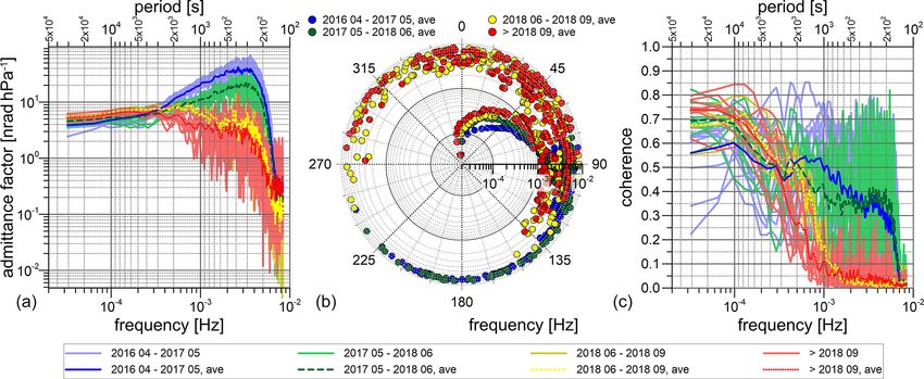
B. Meurers et al.: Hydrological signals in tilt and gravity residuals at Conrad Observatory (Austria)                                           219

Figure 1. Gravitational (Newtonian) tilt and deformation. The sphere represents an arbitrary surplus mass (interior or exterior); lines show
the equipotential surface (blue solid), the planet surface (solid black), the tilt sensor axis (dotted black) and the plumb line (blue dashed).
(a) Initial state, (b) no tilt on a liquid planet, (c, e) tilt due to deformation, (d) Newtonian tilt on a rigid planet, and (f) tilt on a deformable
planet, including both Newtonian tilt and tilt due to surface deformation.

ter (SG) GWR-C025 since 1995 within the framework of the                     hydrogeological contexts. Heavy rain and rapid snowmelt
Global Geodynamics Project (GGP; Crossley et al., 1999)                      cause long-term (a few weeks) residual features, the source
and later the International Geodynamics and Earth Tide Ser-                  of which could not be unambiguously identified so far. The
vice (IGETS; Voigt et al., 2016). After terminating a gravity                installation of two tiltmeters in 2014 provided new insight
time series at Vienna (Austria) extending over 12 years, the                 into possible scenarios of hydrological water transport at CO
SG was moved to the Conrad Observatory (CO, Austria) in                      by comparing tide-free SG and tilt time series, which is sub-
autumn 2007, starting a gravity time series over 11 years that               ject of the investigation subsequently reported.
lasted until November 2018. Looking at the non-tidal contri-
bution to gravity variations revealed a much larger hydrolog-
ical impact on the time series at CO than at Vienna. This is
                                                                             2   Observation site and instrumentation
obviously due to complex water infiltration processes taking
place after long-lasting rain or rapid snowmelt (Mikolaj and
                                                                             The Conrad Observatory is a geophysical–geodynamic re-
Meurers, 2013) because CO is located in a karst area, where
                                                                             search facility located 60 km SW of Vienna (Austria) in a
processes are probably even more complicated than in other
                                                                             carbonate region belonging to the eastern foothill of the East-

https://doi.org/10.5194/hess-25-217-2021                                                       Hydrol. Earth Syst. Sci., 25, 217–236, 2021
220 B. Meurers et al.: Hydrological signals in tilt and gravity residuals at Conrad Observatory (Austria)
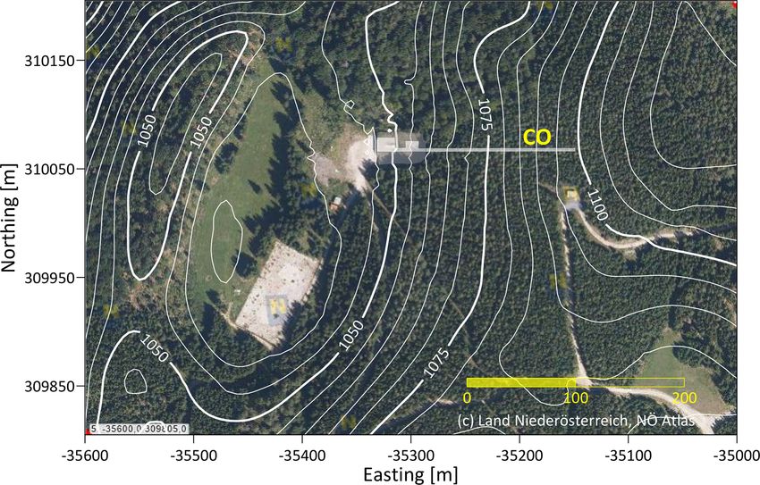
Figure 2. Map of the close surroundings of Conrad Observatory (© Land Niederösterreich, NÖ Atlas). Contour lines represent the topography
elevation (metres) of a high-resolution digital terrain model (DTM) used for modelling. The outline of the observatory, including the 150 m
long tunnel, is displayed as well. Details are presented in Fig. 3.
ern Alps, close to the top of the Trafelberg mountain at tunnel surroundings consist of solid rocks; the coverage in-
an elevation of 1050 m. The Trafelberg mountain itself is creases towards the east from 15 m at the tunnel entrance to
part of the Northern Calcareous Alps and shows a compli- about 55 m at the end, with approximately 33 m at the tilt-
cated nappe structure consisting of Main Dolomite and Wet- meter pier. Given the geometry and orientation of the tunnel,
terstein/Gutenstein limestone (Blaumoser, 2011; Bryda and cavity effects are expected to be the strongest in N–S tilts.
Posch-Trözmüller, 2016). Three karstic caves are known in Gravity data are sampled with 1 Hz by two redundant
the wider surroundings of the observatory (Hartmann and digital volt meters (DVMs) for detecting the possible long-
Hartmann, 2000). No natural springs exist on Trafelberg it- term scale factor changes in the DVMs. SG calibrations
self (Deisl et al., 2014). Therefore, karstic phenomena like by co-located absolute gravimeter (JILAg-6; FG5) observa-
complex underground drainage systems, karst aquifers, caves tions took place twice a year and were supported by numer-
and cavern systems, as well as sinkholes, are expected to ous SG/Scintrex CG-5 relative gravimeter intercomparisons
be present. Figure 2 shows the observatory surroundings. (Meurers, 2012, 2018a). Commonly, the SG scale factor (SF)
The broad local topography low centred 100–200 m west of is assumed constant as long as the hardware (e.g. coil ge-
the observatory probably reflects a sinkhole filled by sedi- ometry and transfer function) does not change (Goodkind,
ments today. Refraction seismic and geoelectric surveys es- 1999), which allows for an averaging of the calibration re-
timate the maximum depth to consolidated rocks to be 30 m sults (Van Camp et al., 2016; Crossley et al., 2018). System-
(Sirri Seren, personal communication, 2012). atic SF changes, if present and larger than 0.1–0.2 ‰, are
The observatory consists of a building (ceiling height of reliably detectable by studying the temporal M2 tidal param-
about 4 m) for offices/laboratories and a 144 m long and 3 m eter modulation of successive tidal analyses over 1 year inter-
wide tunnel drilled in an E–W direction (Fig. 3). In one of the vals. Combining calibration results and M2 parameter modu-
laboratories, a massive concrete pier is directly connected to lation studies (Meurers et al., 2016) proved the accuracy and
solid rock for gravimeter installations. Prior to the construc- time stability of the SG scale factor at CO to be far below
tion of the building, a huge amount of rock was blasted out 1 ‰ (Meurers, 2018a).
of the terrain. Before the concrete foundation plate was made In August 2014, the Geodetic and Geophysical Institute
for the building, the remaining cragged and rough rock sur- (GGI, Sopron, Hungary) installed a 5.5 m long Michelson–
face was levelled by a gravel sheet. After completion of the Gale-type interferometric water level tiltmeter (iWT),
building, the space next to and above the building was re- recording at only one end of the tube, designed by the Finnish
filled by the excavated material in order to restore the original Geodetic Institute (FGI; Ruotsalainen et al., 2016a, b; Ruot-
terrain shape. Above the SG, coverage amounts to approxi- salainen, 2018), on a 6 m long pier in the middle of the tun-
mately 7 m. The gravel sheet below the building is a potential nel, about 94 m away from the SG. Continuous tilt measure-
water storage reservoir influencing the observed gravity. The ments started at CO in order to monitor geodynamical phe-
Hydrol. Earth Syst. Sci., 25, 217–236, 2021 https://doi.org/10.5194/hess-25-217-2021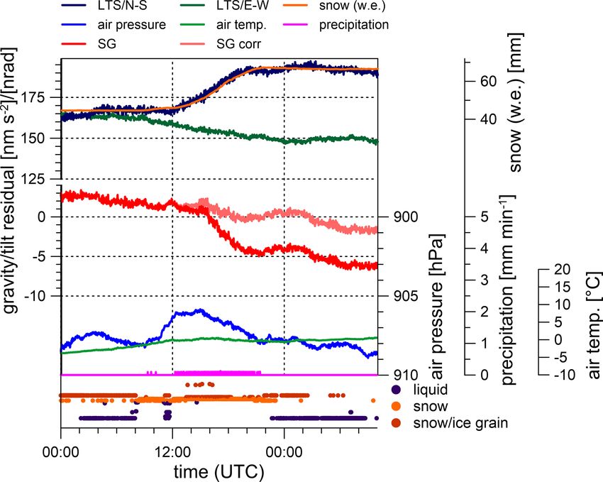
B. Meurers et al.: Hydrological signals in tilt and gravity residuals at Conrad Observatory (Austria)                             221

Figure 3. Vertical section and ground plan of the Conrad Observatory. Sensor positions are displayed by black dots. Small dots indicate
boreholes of different depth.

nomena like microseisms, free oscillations of the Earth, earth              pressure and temperature sensors in the observatory labs
tides, mass loading effects (ocean tidal and atmospheric load-              and the tunnel.
ing) and possible crustal deformations. In July 2015, a Lipp-
mann high-resolution tiltmeter (HRTM) 2D pendulum tilt                    – A tipping bucket rain gauge model AP-23 (Anton Paar
sensor (LTS) with < 1 nrad resolution (https://www.l-gm.de/                 GmbH, Austria) with 0.1 mm resolution.
en/en_tiltmeter.html, last access: 23 November 2020) was in-
stalled by GGI close to the iWT on the same pier (Papp et al.,            – A disdrometer (Adolf Thies GmbH & Co. KG, Ger-
2019). This set-up of instruments based on different physical               many) measuring the size and fall speed of precipita-
principles (relative height change of a level surface vs. in-               tion particles and classifying the precipitation type by
clination change of the plumb line) allows for a comparison                 the surface synoptic observations (SYNOP) code.
of the response of tiltmeters with long (several metres) and
                                                                          – A 3D ultrasonic anemometer                (Adolf     Thies
short (a few decimetres) base lengths. While iWT monitors
                                                                            GmbH & Co. KG, Germany).
E–W tilts, LTS provides both N–S and E–W tilt time series.
The tiltmeter sampling rate is 1 Hz (LTS) and 15 Hz (iWT)                 – A SSG-2 snow scale (Sommer Messtechnik, Austria)
respectively. The scale factor of the LTS tiltmeter is factory              monitoring the weight of the snow pack in front of the
based. The iWT scale factor is absolute and based on optical                observatory and providing snow water equivalent data.
interferometry in the CO station condition. The iWT tiltmeter               The snow scale was out of operation between 1 January
detects crustal tilt from water level variations at one end of              and 15 March 2018. Missing data has been replaced by
the tube by interference phase values, which are converted                  information from a nearby (150 m SW of the observa-
to tilt by a conversion factor based on laser wavelength, re-               tory) snow height sensor.
fraction coefficient of water and tube length of the tiltmeter
(Ruotsalainen, 2018).
   All instruments are underground installations in a ther-           3    Gravity and tilt preprocessing and determination of
mally stable environment. The tiltmeters are located approx-               residuals
imately 33 m below ground surface. Based on theoretical
calculations by Harrison and Herbst (1977), Bonaccorso et             To separate small amplitude gravity and tilt signals of dif-
al. (1999) estimate that the maximum amplitude of thermoe-            ferent physical origins, like, for example, hydrological re-
lastic tilt of the rocks beneath the surface decays towards zero      sponse or tectonic signals, we need to subtract the tidal ef-
at 10 m depth. Even if this approach might underestimate the          fects which dominate the gravity and tilt time series. The
real thermoelastic effect, as shown by experiments with shal-         atmospheric pressure and polar motion are also known to
low borehole tiltmeters at different depth (Bonaccorso et al.,        contribute remarkably to temporal gravity and tilt variations,
1999), the coverage of 33 m should reduce thermoelastic tilt          although much less so than the tides. Both the SG and the
deep in the tunnel.                                                   tiltmeters are relative instruments and, hence, may exhibit
   In order to investigate atmospheric and precipitation ef-          instrumental drift. Generally, the SG drift is expected to be
fects on gravity, a wide range of meteorological parameters           only a few nm s−2 per year. Absolute gravity observations
are monitored by mobile and permanent sensors as follows:             performed at CO did not reveal any significant instrumen-
                                                                      tal drift of the SG until now (Meurers, 2018b). However,
  – The air pressure, air temperature and humidity sensors            the tilt sensors show strong drift dominated by linear trends
    located outside, above the laboratory; an air pressure            up to −10 and +2.5 µrad yr−1 for the LTS and iWT sen-
    sensor included in the SG-acquisition system; the air             sors, respectively, and by possible thermal origin. There-
    pressure, temperature and humidity sensors integrated             fore, the gravity and tilt time series must be properly pro-
    within the LTS tiltmeter housing; and additional air              cessed to derive the residual time series. Preprocessing and

https://doi.org/10.5194/hess-25-217-2021                                              Hydrol. Earth Syst. Sci., 25, 217–236, 2021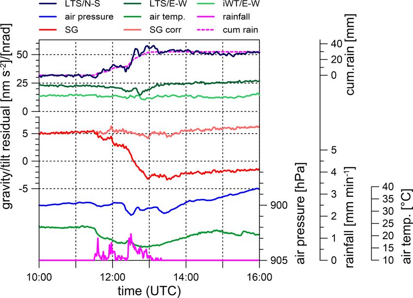
222                  B. Meurers et al.: Hydrological signals in tilt and gravity residuals at Conrad Observatory (Austria)

determination of gravity/tilt residuals followed the proce-        NAO99 in Matsumoto et al., 2000). This is due to the high
dure which is standard for SG time series (Hinderer et al.,        accuracy of both the SG scale factor determination (0.2 ‰)
2007). To decimate the 1 Hz samples to 1 min or 1 h sam-           at CO (Meurers, 2018a) and the tidal analysis, which is based
ples, we applied numerical filters g1s1m and g1m1h, re-            on time series longer than 10 year (Meurers, 2018b). The for-
spectively (http://www.eas.slu.edu/GGP/ggpfilters.html, last       mal errors of gravimetric factors are far below 0.1 ‰ for the
access: 23 November 2020). Local tide models in the diur-          main tidal constituents. The root mean square (RMS) error
nal and sub-diurnal frequency bands and air pressure admit-        of a single observation estimated from the tidal adjustment
tances were derived individually for each sensor from tidal        residuals, which was calculated by using the adjusted tidal
analyses by applying ETERNA v3.4 and ETERNA-x et34-x-              parameters, is 0.6 nm s−2 or 0.9 ‰ of the tidal peak-to-peak
v80 (Wenzel, 1996; Schüller, 2020). Tidal parameters of the-       M2 amplitude only.
oretical body tide models (e.g. Dehant et al., 1999) are used         Local tide models for the tilt sensors are much less accu-
for long-period tides. The following preprocessing steps had       rate. The RMS errors of a single observation derived from
to be applied additionally for the tilt sensors:                   the least squares adjustment (LSQ) of tidal parameters range
                                                                   from 1.6 to 2.9 nrad, which is of the order of about 2 %–
    – Interpolation of 15 Hz iWT data to 5 Hz samples and          4 % of the peak-to-peak M2 tidal signal. Also, much less
      decimation of 5 Hz data to 1 Hz samples by using a           data (LTS N–S – 21 700 hourly samples within 1064 d; SG
      Gaussian operator with 61 coefficients equivalent to         – 83 500 hourly data within 3512 d) could be used for tidal
      1 min time length.                                           analyses. Table 1 compares the tidal parameters of the main
    – Correction of transient signals due to thermal distur-       tidal groups for the LTS and iWT tilt sensors. The LTS N–
      bances in the tunnel, which are very small but hap-          S component turns out to be heavily disturbed by non-tidal
      pen occasionally during maintenance work. Until Au-          excitation, particularly in the diurnal band, while the E–W
      gust 2017, an episodic temperature increase of a few         components do not deviate considerably from the body tide
      0.01 ◦ C inside the LTS was observed by the built-in sen-    predictions. We also analysed the data a priori corrected for
      sor, generating tilt signals much larger than the tidal      atmospheric and induced non-tidal oceanic loading contri-
      signal. The temperature correction was based on linear       butions (Boy et al., 2009) provided by the School and Ob-
      or nonlinear models, depending on the thermal event.         servatory of Earth Sciences (EOST) Loading Service (http://
      Since August 2017 both tilt sensors have been isolated       loading.u-strasbg.fr/, last access: 23 November 2020). After
      from the temperature fluctuation in the tunnel by styro-     correction, the non-tidal tilt anomaly in the diurnal band still
      foam sheet insulation around the tiltmeters, which ef-       persists. However at CO, ocean loading corrections based on
      fectively suppresses the thermal disturbances.               the TPXO9 model (http://holt.oso.chalmers.se/loading/, last
                                                                   access: 23 November 2020) do not essentially reduce the de-
    – Correction of steps, in particular for iWT data, by ap-      viation of the observed tilt factors from the body tide predic-
      plying TSoft (Van Camp and Vauterin, 2005) and our           tions. Because the tunnel axis is oriented in an E–W direc-
      own codes. Due to its incremental measuring princi-          tion, the N–S component corresponds to the tilt perpendicu-
      ple, iWT sometimes suffers from interference phase cy-       lar to the tunnel axis and, therefore, is extremely sensitive to
      cle slips; the correct interpretation of the interferogram   cavity effects (King and Bilham, 1973; Harrison, 1976; Ag-
      phase fails if the phase change between two consecu-         new, 1986). This is the most likely reason for anomalous tidal
      tive interferograms is larger than one interference phase    parameters in the N–S tilt, particularly in the diurnal band
      value, typically of 203.6 nm. This happens during large      where tidal N–S tilt wave amplitudes are small (< 5 nrad).
      earthquakes when ground motion is so fast that the fluid     The high LTS/iWT ratio of the E–W tilt factors hints at cal-
      level of the instrument cannot follow the fast and large     ibration errors. LTS tilt factors are about 6 %–11 % higher
      seismic surface wave arrivals in the first minutes.          than those of the iWT, i.e. the tidal parameters are probably
                                                                   also affected by unknown transfer functions of the tilt sen-
    – Removal of the low-order polynomial trends.
                                                                   sors. However, we cannot exclude the idea that cavity effects
                                                                   play a role as well, as the respective tilt sensors are not at
4     Local tide models and air pressure admittance                exactly the same place and have different base lengths. In or-
                                                                   der to consider all these problems properly, sensor-dependent
The local tide model for gravity matches the theoretical           tidal models have been used for the tilt residual determina-
body tide models (e.g. Dehant et al., 1999; Mathews, 2001)         tion.
and the ocean tide loading predictions provided by Bos and            Air pressure also has a strong impact on observed tilts, pre-
Scherneck (2017) almost perfectly (e.g. CSR4.0 in Eanes,           dominantly due to surface loading (e.g. Rabbel and Zschau,
1994; GOT00.2 in Ray, 1999; TPXO7.2 and TPXO9 in Eg-               1995) and directly results in surface and subsurface de-
bert and Erofeeva, 2002; FES2004 in Lyard et al., 2006;            formation, depending on the spatial scale of load masses
EOT11a in Savcenko and Bosch, 2011; DTU10 in Cheng                 (e.g. Llubes et al., 2004). Air pressure changes are caused by
and Andersen, 2010; HAMTIDE in Taguchi et al., 2014; and           air packages with different densities and spatial extent pass-

Hydrol. Earth Syst. Sci., 25, 217–236, 2021                                          https://doi.org/10.5194/hess-25-217-2021
B. Meurers et al.: Hydrological signals in tilt and gravity residuals at Conrad Observatory (Austria) 223
Table 2. Air pressure admittances in the diurnal and semidiurnal
Table 1. Comparison of tidal parameters derived from tilt time series at CO. Theoretical body tide model as per Dehant et al. (1999). Note: LTS – Lippmann HRTM 2D pendulum tilt frequency band for the tilt sensors derived from tidal analysis.
1.0577
1.0680
1.0762
1.0806
1.1117
1.0775
γ (iWT)
γ (LTS)
Air pressure admittance (nrad hPa−1 )
N–S E–W
−11.349 ± 0.493
−11.244 ± 0.314
−4.449 ± 0.382
−5.525 ± 0.080
−5.015 ± 0.204
−4.875 ± 0.871
LTS LTS iWT
4.247 0.097 −0.475
φ (◦ )
σ (φ)
±0.034 ±0.019 ±0.034
iWT
ing the station. Therefore, air pressure signatures in tilt time
0.6746 ± 0.0058
0.7278 ± 0.0040
0.7130 ± 0.0048
0.6849 ± 0.0010
0.6203 ± 0.0023
0.6385 ± 0.0097
series are expected to be frequency dependent, as it is well
σ (γ )
known from gravity records. Loading by accumulated wa-
γ
ter or snow produces deformation in a similar way. Hence,
it is worth studying the air pressure admittance function for
the tilt. Air pressure tilt admittances for tidal frequencies
E–W
were calculated in a joint adjustment, together with the tidal
parameters by ETERNA-x et34-x-v80 software (Schüller,
−6.902 ± 0.272
−7.615 ± 0.187
−2.495 ± 0.288
−4.102 ± 0.060
−2.676 ± 0.146
−2.577 ± 0.608
2020). The results in Table 2 represent the diurnal and semid-
φ (◦ )
σ (φ)
iurnal frequency band only because long-period tides were
not included in the adjustment. To obtain higher frequency
information, we investigated the frequency dependence of
LTS
the air pressure admittance by applying a cross-spectral anal-
0.7135 ± 0.0034
0.7773 ± 0.0026
0.7673 ± 0.0039
0.7401 ± 0.0008
0.6896 ± 0.0018
0.6880 ± 0.0073
ysis (Bendat and Piersol, 2010) on several detided tilt time
series covering intervals between 2 and 21 d (10 d on aver-
σ (γ )
age) for both LTS N–S and LTS E–W. For LTS N–S, the air
γ
pressure admittances confirm the number resulting from the
tidal analysis (Table 2) obtained in the diurnal and semidiur-
nal frequency band. Clear time variability is seen at frequen-
(nrad)
23.4455
32.9605
9.8359
51.3708
23.8984
6.4926
amptheor
cies beyond 0.3 mHz (equivalent to a period of about 1 h),
which is of instrumental origin. Therefore, separating phys-
ically meaningful signals from instrumental artefacts is not
possible in the frequency range larger than 0.3 mHz. Details
are provided in Appendix A. However, at long periods, the air
φ (◦ )
σ (φ)
7.235 ± 1.867
−1.318 ± 1.152
−2.691 ± 0.579
−3.193 ± 0.115
−2.880 ± 0.264
−2.531 ± 1.116
pressure signal in the tiltmeter time series is due to geophysi-
cal/geodynamical reasons, which are probably dominated by
deformation due to air pressure loading. Here, the admittance
is again much higher for the N–S tilt than for E–W tilt (sim-
ilar to that shown in Table 2), which is as expected due to
sensor; iWT – interferometric water level tiltmeter.
1.0997 ± 0.0358
1.2920 ± 0.0259
0.6648 ± 0.0067
0.6628 ± 0.0013
0.6777 ± 0.0031
0.6612 ± 0.0129
the cavity effect. We will come back to this in Sect. 5.1 when
N–S
LTS
we discuss the tilt response to water mass load on the terrain
σ (γ )
surface.
γ
5 Gravity and tilt residuals at Conrad Observatory
(nrad)
3.1275
4.3962
7.3013
38.1330
17.7398
4.8195
amptheor
Figure 4 presents the final gravity and tilt residuals of
the common observation period extending from end of
April 2016 until mid-November 2018. Comparing the resid-
0.6976
0.7379
0.6945
0.6945
0.6945
0.6945
model
Tide
uals with cumulative rain and snow (water equivalent) shows
γ
an obvious link between both short- and long-term residual
anomalies related to different hydrological processes.
Darwin
symbol
group
Wave
M2
O1
K1
N2
K2
S2
https://doi.org/10.5194/hess-25-217-2021 Hydrol. Earth Syst. Sci., 25, 217–236, 2021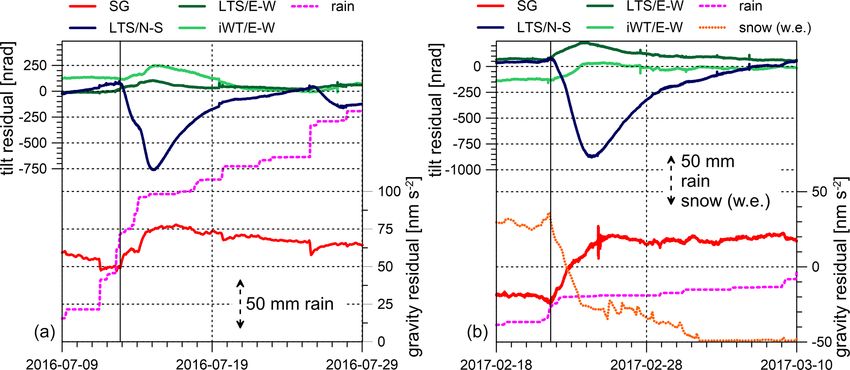
224                  B. Meurers et al.: Hydrological signals in tilt and gravity residuals at Conrad Observatory (Austria)

Figure 4. Comparison of gravity and tilt residuals, showing gravity (red), N–S tilt (LTS – dark blue), E–W tilt (LTS – dark green; iWT –
light green), cumulative rain (dashed magenta line); snow water equivalent (dotted orange line). Scales for rain and snow (water equivalent)
are indicated by arrows. Vertical dotted lines mark the onset of hydrologically induced long-term events.

5.1   Short-term signatures (water accumulation phase)                  mated by multiplying the cumulative rain with a rain admit-
                                                                        tance factor based on a digital terrain model in a high spatial
                                                                        resolution (Meurers et al., 2007). The rain admittance de-
Figure 5 presents a typical example of a heavy rain event on            pends on terrain geometry, SG sensor location and on the
11 July 2016. The SG residuals decrease sharply and exactly             area of rainwater accumulation. At CO, the rain admittance
at the time when rain starts. This is mainly due to the New-            varies between −0.26 and −0.29 nm s−2 per 1 mm rain for
tonian effect of rainwater distributed at the terrain surface,          accumulation areas between 104 and 102 km2 (Fig. 6a). Cor-
above the instrument. Actually, due to their high precision,            recting for the Newtonian effect of cumulative rain removes
SGs reveal these effects not only in the case of heavy rain             the gravity response to rain almost perfectly (Fig. 5; light red
events but also in the case of light rainfall even smaller than         line). Of course, the rain admittance concept works only dur-
1 mm h−1 . The gravity residual drop can be very well esti-

Hydrol. Earth Syst. Sci., 25, 217–236, 2021                                                 https://doi.org/10.5194/hess-25-217-2021
B. Meurers et al.: Hydrological signals in tilt and gravity residuals at Conrad Observatory (Austria)                                 225

                                                                          short-term signatures that could be related to rain. In only
                                                                          10 out of 48 rain events is a slight transient residual decrease
                                                                          visible, which, however, often starts much earlier than rain.
                                                                          Figure 7a shows the observed total N–S tilt offsets as a func-
                                                                          tion of cumulative rain or of the surface pressure load exerted
                                                                          by cumulative rain at the end of the respective rain event. The
                                                                          average rain admittance results in 0.73 nrad mm−1 , which is
                                                                          about 580 times larger than the value estimated for purely
                                                                          gravitational tilt (Fig. 6) or about 7.4 nrad hPa−1 after con-
                                                                          verting cumulative rain into surface load pressure. This cor-
                                                                          responds to the air pressure admittance for the N–S tilt at
                                                                          about 0.3 mHz. Also, we find a close relation between the re-
                                                                          sponse of N–S tilt and gravity to short-term water accumula-
                                                                          tion at topography (Fig. 7b). The air pressure admittances for
                                                                          the E–W sensors are much weaker than those for the N–S tilt
Figure 5. Effect of heavy rain on gravity and tilt at CO on               sensor at all frequencies, which may explain why we rarely
11 July 2016. Gravity and N–S tilt residuals show patterns clearly        see E–W tilt effects due to rain. Surface load (either due to air
related to cumulative rain, while E–W tilts do not, or only weakly,       pressure or rain/snow) rarely produces clear signatures in the
respond to rain. The legend indicates the following, from top to bot-     E–W tilts because the cavity effect is much smaller for E–W
tom: N–S tilt residuals (dark blue), E–W tilt residuals (LTS – dark       tilt than for N–S tilt. Tilt response to surface load by water
green; iWT – light green), cumulative rain (dashed magenta line)          accumulation evidently compares well with the tilt response
scaled to fit the N–S tilt optimally, SG gravity residuals (red), grav-   to atmospheric pressure changes for both the N–S and the
ity corrected for cumulative precipitation (light red), rainfall (ma-
                                                                          E–W components. The SG reflects mainly the gravitational
genta), air pressure (blue) and outdoor air temperature (green).
                                                                          effect of the rain/snow water, while the deformation effect
                                                                          on gravity (vertical displacement) at the given spatial scale
                                                                          is too small to be detected; in contrast, the tiltmeter responds
ing the accumulation phase, while it fails when the residuals             to deformation caused by the pressure the water exerts onto
recover their initial level after rainfall.                               the terrain surface, similarly to in case of air pressure vari-
   The same approach can be applied to estimate the Newto-                ations. It is probably the cavity effect, which amplifies the
nian tilt effect of rainwater in both the N–S and E–W di-                 observed tilt such that it emerges from the noise in case of
rection. Corresponding rain admittances turn out to be as                 the N–S component, which is oriented perpendicular to the
small as −1.3 × 10⁻³ nrad per 1 mm rain for the N–S tilt and              tunnel axis at CO.
−7.6×10⁻³ nrad per 1 mm rain for the E–W tilt, respectively,                  The findings above also hold in the case of solid precipita-
if the rainfall area extends to more than 2 km symmetrically              tion, as shown in Fig. 8, which presents an example of grav-
around the tilt sensor (Fig. 6b). In the case of a rain front, the        ity and N–S tilt response to pure snow accumulation. Dis-
Newtonian effect can be considerably larger and depends on                drometer data (Fig. 8; coloured dots) show that almost no
the direction from which the rain front approaches the sta-               liquid precipitation is involved. The disdrometer provides in-
tion. The effect of asymmetric rainfall areas extending to a              formation on the aggregate state of the precipitation particles
line just passing the tilt sensor location provides the maxi-             even for extremely little precipitation. However, as indicated
mum estimate, which does not exceed ±7.7 × 10⁻² nrad per                  by the rain data (Fig. 8; magenta), liquid rain does not es-
1 mm rain at CO. However, in realistic weather situations,                sentially contribute to water accumulation in the presented
the rain-to-tilt admittance is much smaller and depends on                case study. Consequently, no essential water infiltration can
the velocity at which the rain front moves over the sensor.               take place because most precipitation is solid and air temper-
Given these small numbers, the Newtonian tilt effect of rain-             ature remains slightly below the melting point (Fig. 8; green
water or snow turns out to be negligible at CO because it is              line). Note that heated rain gauges often report solid precipi-
far below the reliable resolution of tiltmeters.                          tation incorrectly and/or time delayed because the solid par-
   Nevertheless, there is a clear and instantaneous N–S tilt              ticles have to melt before they are counted by a bucket rain
response on rain (exemplarily shown by Fig. 5), which is                  gauge. The disdrometer detects precipitation starting as snow
visible in almost all (71 out of 74) heavy rain events. Tilt              grains and light drizzle during night and early morning with
response on air pressure changes can be ruled out as a rea-               an intensity which is too small to be observed by the rain
son because the temporal patterns of air pressure and tilt are            gauge. Precipitation continues as light to heavy snow from
totally different in most cases, while tilt and cumulative rain           08:00 universal coordinated time (UTC) onwards. The snow
match each other. Similar to the case of gravity, we do not               scale indicates the onset of snow cover increase at about
observe any time delay between cumulative rain and tilt re-               12:00 UTC. Gravity residuals start decreasing at the same
sponse. In contrast, tilts in the E–W direction rarely show               time and reach a local minimum at about 22:00 UTC when

https://doi.org/10.5194/hess-25-217-2021                                                  Hydrol. Earth Syst. Sci., 25, 217–236, 2021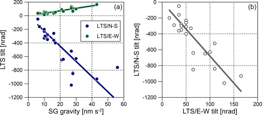
226                   B. Meurers et al.: Hydrological signals in tilt and gravity residuals at Conrad Observatory (Austria)

Figure 6. Modelled gravitational effect of 10 mm rain on gravity (a) and tilt (b) at CO.

Figure 7. Short-term N–S tilt and gravity residuals (water accu-
mulation phase). N–S tilt response to cumulative rain at CO (a).
Converting cumulative rain to surface pressure load reveals a tilt-
to-pressure admittance of 7.6 nrad hPa−1 (solid line). Relation be-
tween gravity and N–S tilt residuals (b).

                                                                         Figure 8. Effect of snow accumulation on gravity and tilt at CO
heavy snow fall terminates. The prediction of the cumula-                on 21 and 22 December 2017. The legend indicates the following,
                                                                         from top to bottom: N–S tilt residuals (dark blue), E–W tilt residu-
tive precipitation effect by applying the rain admittance re-
                                                                         als (dark green), snow (water equivalent – orange) scaled to fit the
moves the gravity residual drop almost perfectly (Fig. 8; light          N–S tilt optimally, SG gravity residuals (red), gravity corrected for
red line). A significant signal associated with the main snow            cumulative precipitation (light red), air pressure (blue) and outdoor
accumulation phase is also visible in the N–S tilt residuals,            air temperature (green).
which are comparable in magnitude to rainfall events (com-
pare to Fig. 5), i.e. snow affects tilts similarly as in the case
of rain, and the snow water equivalent matches the tilt time             5.2    Long-term signatures (water percolation phase)
pattern if properly scaled (Fig. 8; orange line). Again, gravity
and tilt react instantaneously, i.e. without time delay.                 It is common to most rain events that, after rainfall, a slow
   The short-term residual anomalies can therefore be well               discharge process brings the gravity residuals back to their
explained by the accumulation of precipitation on the ter-               initial level (Fig. 4). However, in some events, the residuals
rain surface and in the adjacent topsoil. While the gravity re-          exceed the initial level remarkably, in particular after long-
sponse reflects the gravitational acceleration of accumulated            lasting rain or rapid snowmelt. We interpret this as the re-
water/snow mass, the N–S tilt response is interpretable as               sponse to downward water flow (infiltration) from the terrain
the pure deformation effect caused by the pressure the water             surface into the ground until water is stored somewhere be-
mass exerts on the terrain surface. Similarly, as in the case            low the SG sensor. This process probably starts as soon as the
of atmospheric pressure changes, the cavity effect enhances              subsurface is sufficiently saturated by rain or snowmelt wa-
observed tilts in the N–S direction much more than those ori-            ter and, therefore, needs a certain threshold to be triggered.
ented E–W. If the accumulation phase is short, as in the case            Mangou (2019) estimated that about 20 mm water accumula-
studies discussed so far, we do not expect considerable water            tion within the past 3 d is required. However, this number is a
percolation into the subsurface to change the pore pressure              rough estimate. The degree of saturation and meteorological
there.                                                                   conditions (e.g. evaporation rate, etc.) plays a role as well.

Hydrol. Earth Syst. Sci., 25, 217–236, 2021                                                  https://doi.org/10.5194/hess-25-217-2021
B. Meurers et al.: Hydrological signals in tilt and gravity residuals at Conrad Observatory (Austria) 227
Figure 9. Long-term gravity and tilt residual signals caused by hydrological processes after heavy and long-lasting rain (a) and during
rapid snowmelt (b). N–S tilt residuals (dark blue) and E–W tilt residuals (LTS/dark green and iWT/light green). SG gravity residuals (red).
Cumulative rain (dashed magenta line), snow (water equivalent; dotted orange line). Scales for rain and snow water equivalent indicated by
arrows. The black vertical line shows the onset of the long-term residual anomaly.
Interestingly, all of these events are associated with si-
multaneous long-term tilt anomalies. Almost at the same
time that the SG gravity residual starts to increase, we see
strong signals in the tilt time series as well. The N–S tilt al-
ways shows a steep residual drop, and the E–W tilt residu-
als (in particular LTS) increase temporarily but with much
less amplitude. E–W tilt signals are often masked by noise.
All events in which we identified long-term signatures both
in gravity and tilt residuals are marked by dotted vertical
lines in Fig. 4. Figure 9 exemplarily enlarges into a long-
lasting rain event (Fig. 9a) and into a rapid snowmelt event Figure 10. Long-term tilt (LTS) and gravity residuals (water perco-
lation phase). Relation between the amplitudes of long-term tilt and
(Fig. 9b). Once N–S and E–W tilts have reached their ex-
gravity residual anomalies (a). Relation between the amplitudes of
tremes, they return to their former level; this is a process long-term N–S and E–W tilt residual anomalies (b). The average
which takes about 14 d or more. The short-term signals dis- ratio of N–S to E–W tilt is −0.15.
cussed in Sect. 5.1 are visible in Fig. 4 too, even though
they are very small compared to the long-term signal. The
long-term anomalies start when sufficient water has perco- 6 Discussion
lated downwards into the subsurface, either after heavy/long-
lasting rainfall or in case of rapid snowmelt. Quantifying the In the following, there are a few candidates for water storage
long-term anomalies is not easy because the tilt/gravity re- volumes at CO:
sponse to long-term water transport depends on the over- – the gravel layer below the concrete foundation plate of
all subsurface saturation for which we have no constraints the underground observatory building and the laborato-
based on observations. However, there is a significant rela- ries in front of the tunnel,
tion between the long-term residual anomalies observed in
the tilt and gravity residuals (Fig. 10a). Tilt residual anoma- – fissures and cracks in the solid rock, or
lies always have either negative (N–S tilt) or positive (E–
– perhaps a karstic volume filled by water after heavy
W tilt) signs. The absolute value of the anomaly ampli-
rain/snowmelt.
tudes increases with the amplitude of the gravity residual
anomaly, whereby the N–S residual anomaly amplitude is We first investigate whether a locally limited surface or
about 7 times larger on average than that of E–W residuals subsurface mass is able to produce the observed long-term
(Fig. 10b). tilt/gravity residuals. Comparing the E–W and N–S tilt data,
the amplitude ratio of the long-term residual anomalies turns
out to be about −0.15 on average (Fig. 10b). E–W tilt is al-
ways positive; N–S tilt is always negative (Fig. 10a). If the
observed tilt is solely due to gravitational attraction by a vol-
ume of stored water, then the source must be located on a line
https://doi.org/10.5194/hess-25-217-2021 Hydrol. Earth Syst. Sci., 25, 217–236, 2021228 B. Meurers et al.: Hydrological signals in tilt and gravity residuals at Conrad Observatory (Austria)
Figure 11. Estimation of the magnitude of water volume (black)
capable of producing 1 nrad tilt if it was purely Newtonian. The
dotted line shows the cross section of the topography in the specific Figure 12. Modelled gravity of a layer with constant thickness as
azimuth defined by the E–W and N–S tilts detected during rainfall function of the layer thickness and the degree of initial soil/rock
events. saturation (for an explanation, see the text).
with an azimuth of about 170◦ . Based on the high-resolution – model calculations show that, contrary to the short-term
digital terrain model (DTM) of the area (Meurers et al., anomalies, no reasonable solution exists to explain the
2007), the existence of any surface depression capable of cu- observed long-term tilt and gravity effects, and
mulating enough run-off water mass (Kalmár and Benedek,
2018) to generate the observed tilts can be checked. Fig- – the onsets of the long-term residual features in gravity
ure 11 shows that there are two local topographical lows (val- and tilt do not coincide exactly in time.
leys) along the profile. However, due to their distances from
Deformation by increasing pore pressure after water infil-
the observatory, an enormous amount of water (> 105 m3 )
tration into the subsurface is the most reasonable explana-
would have to be accumulated in a corresponding cell of the
tion for the observed tilts. Actually, the observed long-term
DTM (determined by the azimuth) to generate even a fraction
N–S tilt response (Figs. 4 and 9) is very similar in shape
(1 nrad) of the observed tilts (up to ∼ 1000 nrad). Regard-
to the observations reported by Herbst (1979) or by Jahr et
ing the horizontal extension of such a cell (50 m × 50 m), a
al. (2006a, b) in one of the tilt records of a borehole tiltmeter
40 m water height would be required to provide this volume.
array established at the KTB deep drilling site (Germany).
The same holds for a fictitious topographical reservoir lo-
Certainly, the hydrological water transport process is very
cated in the very close vicinity (< 50 m) since about 1000 m3
complex at CO. Due to the high sensitivity and extremely
of water is necessary for the same tiny (1 nrad) gravitational
low and almost linear instrumental drift of SG sensors, the
tilt. This volume of water is supplied by 1 mm of rainfall on
SG gravity residual very clearly reveals the Newtonian effect
1 km2 , but obviously even this amount cannot be caught and
(vertical component) of the water mass transport involved in
concentrated near to the observatory, as one can conclude
hydrological charge and discharge processes. We modelled
from Fig. 2 which shows the elevation contour lines. The es-
the gravity effect by a simple layer in order to estimate the
timations above are based on forward gravitational modelling
maximum observable gravity residual drop as a function of
of the horizontal attraction of mass columns (e.g. Papp and
the layer thickness and of the degree of initial soil/rock sat-
Benedek, 2000) representing the water mass placed on top of
uration. The upper layer boundary coincides with the terrain
the topographic mass columns. However, there is no evidence
surface; the lower boundary is defined by shifting the terrain
of such a large basin next to CO in the required azimuth.
surface vertically downwards. The topography is represented
Another point the source modelling shows is that along this
by the same DTM with a high spatial resolution, in particu-
azimuth no spherical volumes representing one single sub-
lar in the vicinity of the SG, as already has been used for the
surface cavity either partially or completely filled by water
rain admittance calculations. The effective layer density δρ
would simultaneously explain both the gravity and tilt resid-
results from Eq. (1) as follows:
uals of the events shown in Fig. 4.
Therefore, regarding the long-term residual variations, a δρ = φ (S − S0 ) ρw , (1)
pure Newtonian effect of one single source (e.g. one single
karstic cave filled by water) representing the water accumula- with ρw and φ denoting water density and rock porosity,
tion near the gravity and tilt sensors can be ruled out because respectively. S0 and S describe the saturation of the pore
of the following two reasons: volume before (initial saturation) and after downward water
mass transport. The model takes into account that water stor-
age is impossible within the volume occupied by the observa-
tory building/tunnel, the foundation plate of the building and
Hydrol. Earth Syst. Sci., 25, 217–236, 2021 https://doi.org/10.5194/hess-25-217-2021B. Meurers et al.: Hydrological signals in tilt and gravity residuals at Conrad Observatory (Austria) 229
Figure 13. Modelled gravity response for a real cumulative rain function (monitored between 11 and 14 July 2016) for different degrees of
initial saturation S0 . Model response (a) and model mismatch (b). Observed gravity (red), cumulative rain (magenta) and gravity effect of
cumulative rain (orange) are shown for comparison. Black vertical lines indicate the onset of the long-term anomaly. The right panel displays
results only for the best-fitting models (0.94 ≤ S0 ≤ 0.96) and for S0 = 0 and S0 = 0.99.
the gravimeter pier. Figure 12 shows the modelled gravity as density δρ, according to Eq. (1). That means that the
a function of layer thickness for S = 1 and different degrees water percolating downwards fills the pore volume com-
of initial saturation S0 , assuming a porosity of φ = 0.1. The pletely. The choice of the porosity seems to be reason-
effective layer density is 100 kg m−3 for initially completely able. Jacob et al. (2009) report values between 0.04
dry rock (S0 = 0). Alternatively, we can interpret Fig. 12 also and 0.12 in a karstic environment (Larzac plateau,
as the gravity effect of the same layers as a function of layer France).
thickness but for different porosity, assuming S = 1 and S0 =
0. Then, the layer density provided in the legend of Fig. 12 – Rainwater is assumed to percolate into the subsurface as
translates into porosity after division by 1000. The minimum a layer of spatially constant thickness H (t). The upper
gravity residual occurs at a layer thickness of about 9 m in layer boundary coincides with the terrain surface as be-
each case, whereby the drop in amplitude increases with fore, while the lower boundary results from shifting the
decreasing degree of initial saturation S0 . Given the terrain terrain surface vertically downwards.
model geometry at CO, the minimum residual drop in ampli-
– The subsurface is partially saturated with a degree of
tude never exceeds about 200 nm s−2 (S = 1 and S0 = 0) at
saturation S0 at the beginning, i.e. before the rain series
the SG site. However, observed numbers are much smaller.
starts.
For all events shown in Fig. 4, the residuals never drop by
more than about 10 nm s−2 , which indicates a high degree – Based on the mass conservation principle, the model
of initial subsurface saturation or porosity lower than as- keeps the balance between accumulated water hw (t) and
sumed in the model. We investigated the period from 11 and the water percolated into the subsurface. This defines
14 July 2016 (Fig. 9a), during which a series of consecutive the thickness of the water layer H as function of time t
heavy or long-lasting rainfall events occurred, in more de- as follows:
tail. Simultaneous to the first rainfall on 11 July 2016, the
gravity residuals decreased by about 8 nm s−2 and remained ρw hw (t)
H (t) = hw (t) = or
nearly at this level after rain has stopped. More heavy rain δρ φ (S − S0 )
events followed, separated by a couple of hours (Fig. 13a). hw (t)
H (t) = for S = 1, (2)
The residuals always drop instantaneously at the onset of φ (1 − S0 )
each event but start to increase a short time later. In total,
they increase to a much higher level than what they started where hw (t) denotes cumulative rain and t = 0 the be-
from at the beginning, although more and more rain is accu- ginning of the first rain event.
mulated. We developed a time-lapse model and compared the
– Water cannot be stored below a maximum layer thick-
time-dependant model response with observed gravity resid-
ness Hs but disappears from there due to any run-off
uals. Unfortunately, we cannot constrain our model by hydro-
process. This constrains the maximum level that the
logical observations. Therefore, the very simplistic model is
gravity residuals can ever reach.
based on the following assumptions:
– If the layer thickness is less than Hs by the end of
– A constant porosity of φ = 0.1 and a constant degree the rain event series, the lower boundary continues
of saturation S = 1, which translates into a subsurface propagating into depth until the layer thickness has
https://doi.org/10.5194/hess-25-217-2021 Hydrol. Earth Syst. Sci., 25, 217–236, 2021230 B. Meurers et al.: Hydrological signals in tilt and gravity residuals at Conrad Observatory (Austria)
reached Hs . However, now the layer thickness increases can distinguish between the following two hydrological pro-
at the expense of layer density (or of saturation S) in cesses:
order to conserve the total water mass. This assumption
considers the general characteristics of the relation be- – Charge process – deformation caused by the surface
tween long-lasting rainfall or heavy rain and residual load (rainwater and snow) produces short-term tilt
gravity: gravity residuals drop down at first, as expected anomalies associated with heavy precipitation.
for underground installations, but later start to increase – Discharge process – deformation probably caused by
and continue increasing even after the rain has stopped pressure changes in the adjacent fracture system induces
at the end of a rain event or rain event series. Figure 9a long-term tilt anomalies lasting over up to 3 weeks.
provides a typical example.
In both cases, tilts in the N–S direction are enhanced due to
Figure 13a shows the modelled gravity response to a real the cavity effect. These hydrological processes, either wa-
cumulative rain function, monitored between 11 July and 14 ter accumulation at the terrain surface (short term) or sub-
July 2016, for a different degree of initial saturation S0 . All surface infiltration (long term), link gravity and tilt resid-
models with S0 ≤ 0.9 clearly fail as they are not able to ex- ual anomalies. Gravity and tilt respond to these processes
plain the overall gravity residual increase during the rain- based on different physical phenomena, namely the gravi-
fall series. Best results are provided for 0.94 ≤ S0 ≤ 0.96, tational effects of moving water mass (gravity) vs. deforma-
with a model misfit (standard deviation) ranging between tion due to loading (tilt). The cavity effect enhances the tilt
3 nm s−2 (S0 = 0.95) and 5 nm s−2 (Fig. 13b). For models component perpendicular to the tunnel axis due to strain–
assuming S0 ≤ 0.9, the misfit standard deviation increases to tilt coupling. Presently, it is not yet clear if karstic phenom-
about 19 nm s−2 . If the subsurface is initially dry (S0 = 0), ena play an important role at CO as well. No large caves are
then the model response (Fig. 13; dark green line) is almost known in the rock massif on which the CO is located. How-
identical to the gravity effect of cumulative rain calculated ever, we cannot exclude that deformation by internal loading
by applying the admittance concept (Fig. 13; orange line), could take place, e.g. when an eventually existing cave or
i.e. all water remains concentrated close to the surface for drainage system is filled by water during hydrological dis-
long time. The key point is that the lower layer boundary has charge (e.g. Tenze et al., 2012).
to propagate downwards fast enough to store water below
the SG sensor. The model is sensitive to the choice of input
parameters like porosity φ or layer thickness Hs . We obtain 7 Conclusion
the same H (t) as long as the denominator is kept constant
Gravimeters provide the integral effect of water storage
in Eq. (2); that is, we can play S0 off against φ. For exam-
changes. The distinct gravity residual anomalies after heavy
ple, the choice of φ = 0.05, which is still reasonable for a
or long-lasting rain and snowmelt have been observed at CO
limestone environment, and S0 = 0.9 would not change the
for long time, and their reason was unclear. Very local water
model response. However, if S0 is 0.5, then porosity has to
storage just below the observatory building after rapid flow
be 0.01, which is very low. Of course, we have to empha-
of surface water through the backfill material on top and be-
sise the simplicity of the model, which, for example, does
side the observatory was the preferred explanation so far. The
not allow for horizontal water flow (e.g. Krause et al., 2009)
tiltmeter instrumentation, initially established for completely
or a direct transport downwards along specific flow paths as
different research goals, has brought new insight to the wa-
expected in karst. Nevertheless, these model results indicate
ter transport processes at CO. The close link between the
that the saturation seems to be high (> 0.9) or that the poros-
long-term gravity and tilt residual anomalies indicates that
ity is low at CO. Note that the model implicitly contains the
the discharge process takes place in a much larger spatial
sinkhole SW from the observatory, at least partly. Based on
context. Simplistic models of uniform water infiltration are
the results from refraction seismic and geoelectric measure-
able to explain the observed gravity residual increase follow-
ments, 3D modelling predicts an additional gravity increase
ing heavy or long-lasting rain. Stepping into even more com-
of only about 4 nm s−2 if porosity of 0.3 and full saturation
plex quantitative modelling certainly requires full hydrolog-
is assumed for the sinkhole filling. However, this small effect
ical equipment (soil moisture, ground water, etc.) in order to
does not change the conclusion drawn from Fig. 13.
constrain the models. Complementary geophysical investiga-
On the contrary, the tiltmeters are not able to capture the
tions like 4D geoelectric monitoring (e.g. Watlet et al., 2018)
gravitational tilt effect because it is too small and thus hid-
and cross-correlation of ambient seismic noise, both of which
den in the noise. However, the N–S tilt residuals in partic-
can provide further information on temporal water saturation
ular show significant, both short- and long-term, anomalies
changes (Fores et al., 2018), are promising techniques for fu-
which are associated with the same rain or snowmelt events
ture investigations.
and are clearly related to the residual patterns captured by
the SG gravity record. Therefore, we explain the tilt resid-
ual anomalies as surface or subsurface deformation. Here we
Hydrol. Earth Syst. Sci., 25, 217–236, 2021 https://doi.org/10.5194/hess-25-217-2021You can also read