Understanding balloon-borne frost point hygrometer measurements after contamination by mixed-phase clouds - AMT
←
→
Page content transcription
If your browser does not render page correctly, please read the page content below
Atmos. Meas. Tech., 14, 239–268, 2021
https://doi.org/10.5194/amt-14-239-2021
© Author(s) 2021. This work is distributed under
the Creative Commons Attribution 4.0 License.

Understanding balloon-borne frost point hygrometer measurements
after contamination by mixed-phase clouds
Teresa Jorge1 , Simone Brunamonti1 , Yann Poltera1 , Frank G. Wienhold1 , Bei P. Luo1 , Peter Oelsner2 ,
Sreeharsha Hanumanthu3 , Bhupendra B. Singh4,5 , Susanne Körner2 , Ruud Dirksen2 , Manish Naja6 ,
Suvarna Fadnavis4 , and Thomas Peter1
1 Instituteof Atmospheric and Climate Science, ETH Zürich, Zürich, Switzerland
2 Deutscher  Wetterdienst (DWD)/GCOS Reference Upper Air Network (GRUAN) Lead Center, Lindenberg, Germany
3 Forschungzentrum Jülich (FZJ), Institute of Energy and Climate Research, Stratosphere (IEK-7), Jülich, Germany
4 Centre for Climate Change Research, Indian Institute of Tropical Meteorology (IITM), Pune, MoES, India
5 Department of Geophysics, Banaras Hindu University, Varanasi, India
6 Atmospheric Science Division, Aryabhatta Research Institute of Observational Sciences (ARIES), Nainital, India

Correspondence: Teresa Jorge (teresa.jorge@env.ethz.ch)

Received: 4 May 2020 – Discussion started: 29 May 2020
Revised: 19 October 2020 – Accepted: 6 November 2020 – Published: 14 January 2021

Abstract. Balloon-borne water vapour measurements in the         outgassing from the balloon and payload, revealing that the
upper troposphere and lower stratosphere (UTLS) by means         latter starts playing a role only during ascent at high altitudes
of frost point hygrometers provide important information on      (p < 20 hPa).
air chemistry and climate. However, the risk of contamina-
tion from sublimating hydrometeors collected by the intake
tube may render these measurements unusable, particularly
after crossing low clouds containing supercooled droplets.       1   Introduction
A large set of (sub)tropical measurements during the 2016–
2017 StratoClim balloon campaigns at the southern slopes         Sources of contamination for cryogenic frost point
of the Himalayas allows us to perform an in-depth analy-         hygrometers are water vapour outgassing from the balloon
sis of this type of contamination. We investigate the effi-      envelope, the parachute, the nylon cord, or sublimation
ciency of wall contact and freezing of supercooled droplets in   of hydrometeors collected in the intake tube of the
the intake tube and the subsequent sublimation in the UTLS       instrument (Hall et al., 2016; Vömel et al., 2016). These are
using computational fluid dynamics (CFD). We find that the       contamination sources common to all balloon-borne water
airflow can enter the intake tube with impact angles up to       vapour measurement techniques (Goodman and Chleck,
60◦ , owing to the pendulum motion of the payload. Super-        1971; Vömel et al., 2007c; Khaykin et al., 2013). The
cooled droplets with radii > 70 µm, as they frequently occur     relative impact of contamination on the measurements in
in mid-tropospheric clouds, typically undergo contact freez-     the stratosphere is severe since the environmental water
ing when entering the intake tube, whereas only about 50 %       vapour mixing ratios are 2–3 orders of magnitude smaller
of droplets with 10 µm radius freeze, and droplets < 5 µm ra-    than in the troposphere. Over time, contamination by
dius mostly avoid contact. According to CFD, sublimation         the flight train (balloon, parachute, nylon cord) has been
of water from an icy intake can account for the occasion-        reduced by increasing the length of the cord by means
ally observed unrealistically high water vapour mixing ratios    of an unwinder and by giving preference to descent over
(χH2 O > 100 ppmv) in the stratosphere. Furthermore, we use      ascent data (Mastenbrook and Dinger, 1961; Mastenbrook,
CFD to differentiate between stratospheric water vapour con-     1965, 1968; Mastenbrook and Oltmans, 1983; Oltmans
tamination by an icy intake tube and contamination caused by     and Hofmann, 1995; Vömel et al., 1995; Oltmans et al.,
                                                                 2000; Khaykin et al., 2013; Hall et al., 2016). Standard

Published by Copernicus Publications on behalf of the European Geosciences Union.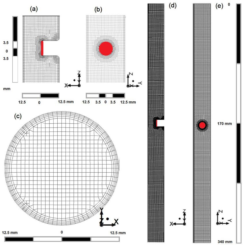
240                                    T. Jorge et al.: Understanding balloon-borne frost point hygrometer measurements

lengths presently used are of the order of 50 to 60 m             the centre of the tube, 17 cm from the opening of the intake
(Vömel et al., 2016; Brunamonti et al., 2018). The World          tube.
Meteorological Organization recommends thin hydrophobic              New designs of frost point hygrometers such as the
tethers longer than 40 m (WMO, 2018; Immler et al., 2010).        SnowWhite sonde from Meteolabor steered away from the
Nevertheless, it has been shown (Kräuchi et al., 2016) that       intake tube design (Fujiwara et al., 2003; Vömel et al.,
the balloon wake in combination with the swinging motion          2003). However, the SnowWhite design was shown to be
of the payload leaves a quasi-periodic signal even in the         susceptible to the ingress of hydrometeors in the intake
temperature measurements by radiosondes. Descent data are         (Cirisan et al., 2014). Under supersaturated conditions, the
not always an option because some instrument intakes and          intake duct was actively heated, with the intention to measure
control systems are optimized for ascent (Kämpfer, 2013).         the total water content (TWC), i.e. gaseous plus particulate
   The first water vapour measurements in the stratosphere        H2 O, instead of just gaseous H2 O mixing ratio, as claimed
were performed by means of a frost point hygrometer               by the manufacturer (Vaughan et al., 2005). The SnowWhite
onboard an aircraft. The reported frost point temperature         sonde was also reported to measure saturation over ice in the
was about −83 ◦ C at 12 km height (Brewer et al., 1948).          troposphere of 120 %–140 %, which could not be modelled
Frost point hygrometers were then developed for balloon-          irrespective of the assumed scenario, leading Cirisan et al.
borne platforms. The first water vapour measurement from          (2014) to conclude the measurement was erroneous and
balloon-borne frost point hygrometers reported a frost point      likely created by contamination.
temperature of about −70 ◦ C at 15 hPa (Barret et al.,               With the increasing miniaturization and ease of use,
1949, 1950; Suomi and Barrett, 1952), corresponding to            balloon-borne frost point hygrometers started to be employed
unrealistically high H2 O mixing ratios (> 100 ppmv). Later,      more systematically at an increasing number of locations
Mastenbrook and Dinger (1961) used a new lightweight              and under a wide range of meteorological conditions (Vömel
dew point instrument for frost point measurements in the          et al., 2002, 2007b; Bian et al., 2012; Hall et al., 2016;
stratosphere. For the first time, measures to minimize            Brunamonti et al., 2018), creating new challenges for the
contamination of the air sample with moisture carried aloft       instrument. When passing through mixed-phase clouds with
by the balloon were mentioned. The instrument was carried         supercooled liquid droplets, the balloon and payload surfaces
about 275 m below the balloon assembly and the ascent             can accumulate ice, which will sublimate in the subsaturated
data were accepted only if validated by the descent data.         environment of the stratosphere. Intake tubes might represent
The descent was achieved by two methods: the use of a             a susceptible surface for this type of contamination (Vömel
big parachute or the use of a tandem balloon assembly.            et al., 2016).
Nowadays, controlled descent profiles are obtained by using          Contaminated water vapour measurements in the strato-
a valve in the balloon neck (Hall et al., 2016; Kräuchi et al.,   sphere are a common feature when the troposphere is very
2016) that slowly releases gas from the balloon. Nearly           moist, such as during deep convection in mid latitudes
all balloon-borne frost point hygrometer (FPH) soundings          (the Asian and North American monsoons) and in the
performed by NOAA’s Global Monitoring Laboratory (Hall            tropics (Holger Vömel, personal communication, 2016).
et al., 2016) use this valve.                                     Contamination requires a careful quality check of the
   Mastenbrook (1965, 1968) identified contamination by           Cryogenic Frost point Hygrometer (CFH) data, representing
the instrument package as a source of the higher and more         a source of uncertainty, especially in the lower stratosphere.
variable concentrations of water vapour at stratospheric          This artifact can also lead to systematic biases, as it
levels. The surfaces of the sensing cavities and intake           makes the operator prefer dryer launching conditions, which
ducts were considered as a potential contamination source         can affect satellite validation procedures and climatological
and redesigned using larger diameter stainless steel intake       records (Vömel et al., 2007a).
tubes that allow higher flow rates. These improvements               During the 2016–2017 StratoClim balloon campaigns at
enabled the instrument to measure typical stratospheric H2 O      the southern slopes of the Himalayas, 43 out of a total of
mixing ratios of about 4 ppmv. Mastenbrook (1966) started         63 soundings carried water vapour measurements by means
building fully symmetric instruments for ascent and descent.      of the CFH (see Vömel et al., 2007b, 2016), and of these 9
Mastenbrook and Oltmans (1983) paid particular attention to       showed strongly contaminated water vapour measurements
the intake tubes of the frost point hygrometer. These tubes       in the stratosphere. These nine soundings are shown in
are currently 2.5 cm in diameter and are made of 25 µm thick      Fig. 1 (see also grey points in Fig. 2 of Brunamonti et al.,
stainless steel (Vömel et al., 2007b). The tubes need to be       2019). The contaminated profiles of the CFH soundings are
thoroughly cleaned before flight. They extend above and           displayed by black lines, while the season average profile,
below the instrument package by more than 15 cm, shielding        excluding the contaminated profiles, as shown in Brunamonti
the air flowing into the instrument from contamination by         et al. (2018) are shown by the grey line. Above 20 hPa
water outgassing from the instrument’s Styrofoam box. The         the season average profile is also considered contaminated,
frost point temperature is measured at the mirror surface         possibly due to water outgassing from the balloon envelope.
displaced 1.25 cm from the intake tube wall and placed at         The values are nonetheless shown in Fig. 1 and marked with

Atmos. Meas. Tech., 14, 239–268, 2021                                               https://doi.org/10.5194/amt-14-239-2021
T. Jorge et al.: Understanding balloon-borne frost point hygrometer measurements                                                        241

Figure 1. Nine water vapour mixing ratio profiles from the CFH showing contaminated values in the stratosphere (out of 43 profiles taken
during StratoClim 16/17). (a–e) Campaign in Naintal (NT), India, summer 2016. (f–i) Campaign in Dhulikhel (DK), Nepal, summer 2017.
Black lines: measured individual profiles. Grey lines: respective campaign season average (mean of 22 (NT) or 7 (DK) profiles), excluding
the individual profiles presented here as contaminated, as shown in Brunamonti et al. (2018). Grey shading highlights possible balloon
contamination above the 20 hPa level in the season average. Two spikes per profile: instrumental clearing and freezing cycles. Highlighted in
red: three night-time launches with the CFH and the COBALD, which are further investigated in this study.

grey shading. Three of the nine contaminated CFH soundings               and operation recommendations to decrease the effect of
also carried the COmpact Backscatter AerosoL Detector                    contamination.
(COBALD) (Wienhold, 2008), namely NT007, NT011 and
NT029.
   Here, we analyse these three soundings thoroughly for                 2     StratoClim balloon campaigns
contamination due to supercooled droplets impacting inside
                                                                         Brunamonti et al. (2018) offer an overview of the
the intake tube during mixed-phase clouds and subsequent
                                                                         instrumentation and dataset collected during the 2016–2017
sublimation of the formed ice layer in the upper troposphere
                                                                         StratoClim balloon campaigns at the southern slopes of
and lower stratosphere (UTLS). We also investigate the
                                                                         the Himalayas, deriving a comprehensive understanding of
balloon envelope and instrument box as possible sources
                                                                         the morphology and large-scale dynamics of the Asian
of contamination. In Sect. 2, we present the dataset
                                                                         Summer Monsoon Anticyclone (ASMA). Here, we focus
and instruments and analyse the mixed-phase clouds. In
                                                                         on humidity measurements in the upper troposphere and
Sect. 3, we describe balloon trajectories and estimate the
                                                                         lower stratosphere region, including the measurement of
impact angles of supercooled droplets onto the tops of
                                                                         mixed-phase and ice clouds, and provide brief instrument
the intake tubes. Section 4 introduces the computational
                                                                         descriptions.
fluid dynamic (CFD) tool FLUENT by ANSYS (2012). In
Sect. 5, we present the results of the different CFD studies,            2.1    CFH and RS41 water vapour measurements
namely Sect. 5.1 for the freezing efficiency of supercooled
droplets; Sect. 5.2 for the CFD-based description of the                 The two instruments measuring water vapour content in this
sublimation process and the evolution of the ice layer;                  study were the radiosonde RS41-SGP (hereinafter referred
Sect. 5.3 for the implications for the measurements in                   to as “RS41”) manufactured by Vaisala, Finland (Vaisala,
the upper troposphere; and Sect. 5.4 for the simulation                  2013), and the Cryogenic Frost point Hygrometer, CFH
of the contamination stemming from the balloon envelope                  (Vömel et al., 2007c, 2016), manufactured by ENSCI (USA).
and instrument packaging. Finally, Sect. 6 provides design               The RS41 measures relative humidity (RH) by means

https://doi.org/10.5194/amt-14-239-2021                                                        Atmos. Meas. Tech., 14, 239–268, 2021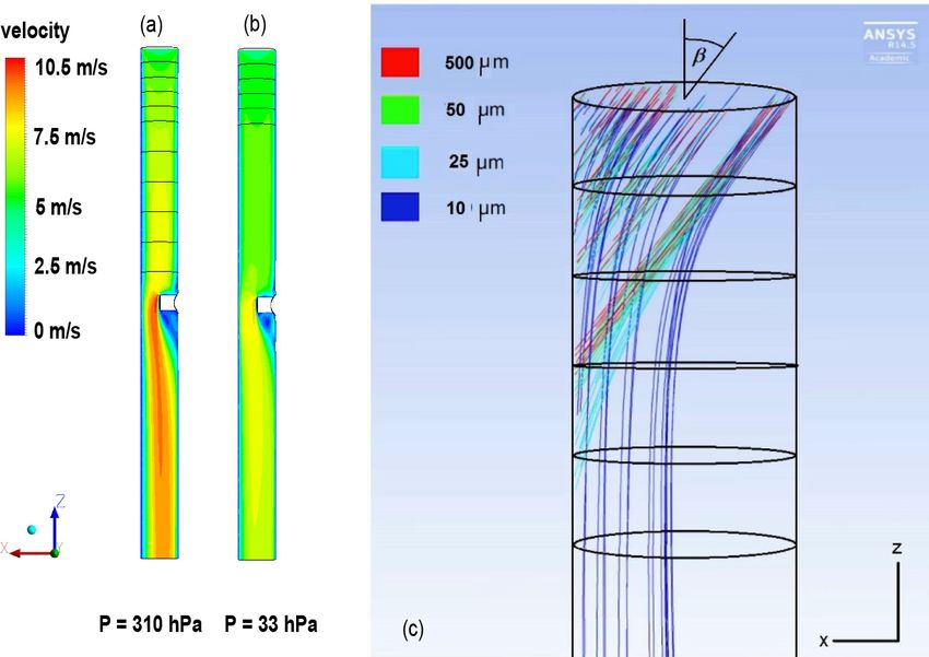
242                                      T. Jorge et al.: Understanding balloon-borne frost point hygrometer measurements

of a thin-film capacitive sensor (Jachowicz and Senturia,            more stable than cubic ice. The data collected during the
1981) with a nominal uncertainty in soundings of 4 % for             freezing and clearing cycles are not used for further analysis,
temperature T > −60 ◦ C (Vaisala, 2013). In this study, we           but we do not remove them from the water vapour profiles.
used corrected RH data provided by the Vaisala MW41                  This feature gives us confidence that after it the phase of the
software for the RS41 measurement, which implements an               deposit in the mirror was ice or hexagonal ice.
empirical time lag correction, accounting for the operation of          We compared the dew- and frost-related quantities (dew
the capacitive sensor under heated conditions by 1T = 5 K            and frost points, corresponding RHs, mixing ratios) of the
above ambient temperature and correcting for irregularities          CFH and RS41 as follows. The ice saturation ratio Sice , i.e.
determined by the zero humidity automated ground check               relative humidity with respect to ice, was calculated using
(Vaisala, 2013). In contrast to the RS41, the CFH measures           the frost point temperature measured by the CFH, the air
the frost point temperature (Tfrost ). It controls the reflectance   temperature measured by the RS41, and the parameterization
of a dew or frost layer on a mirror by heating against               for saturation vapour pressure over ice by Murphy and Koop
continuous cooling of the mirror by a cryogenic liquid. When         (2005), while relative humidity with respect to liquid water
the dew or frost layer is in equilibrium with the air flowing        (Sliq,RS41 , also sometimes simply termed “RH”) was directly
past the mirror, i.e. neither growing nor evaporating, it is by      measured by the RS41. We also present relative humidity
definition at the dew point or frost point temperature, which        (Sliq ) computed from the CFH frost point temperature, the
is a direct measure of the H2 O partial pressure in the gas          RS41 air temperature and the parameterization for saturation
phase. The uncertainty of the CFH has been estimated to              vapour pressure over water by Murphy and Koop (2005).
be smaller than 10 % in water vapour mixing ratio up to              Sliq,d considers the deposit on the CFH mirror to be dew, i.e.
approximately 28 km altitude (Vömel et al., 2007c, 2016).            liquid water, and Sliq,f considers the deposit to be frost, i.e.
   The performance of the two instruments during the 2016–           ice. Water vapour mixing ratio (χCFH ) in ppmv from the CFH
2017 StratoClim balloon campaigns has been thoroughly                was calculated from the frost (or dew) point temperature,
compared, and dry biases of 3 %–6 % (0.1–0.5 ppmv) for               the air pressure from the RS41 and the parameterization
80–120 hPa and 9 % (0.4 ppmv) for 60–80 hPa of the RS41              for saturation vapour pressure over ice (or liquid water) by
compared to the CFH were found. The study uses Vaisala-              Murphy and Koop (2005). The water vapour mixing ratio
corrected RS41 RH measurements (Brunamonti et al.,                   in ppmv derived from the RS41 (χRS41 ) uses the relative
2019). These were campaign mean results, whereas flight-             humidity, air temperature, and air pressure from the RS41
by-flight discrepancies as large as 50 % did occur. In               and the parameterization for saturation vapour pressure over
previous publications of this dataset (Brunamonti et al.,            water by Hardy (1998) as used by Vaisala (2013).
2018, 2019), contaminated measurements in the stratosphere              All data presented were taken during balloon ascent,
were discarded using an empirical threshold. In particular,          because this was the part of the flight affected by
all data above the cold-point tropopause (CPT) were flagged          contamination. We averaged all data in 1 hPa intervals (bins)
as contaminated if H2 O mixing ratios exceeded 10 ppmv               from the ground to the burst altitude. The downward-looking
at any altitude in the stratosphere. In addition, all data           intake did not get contaminated by hydrometeors during
at pressures below 20 hPa were also discarded, due to                mixed-phase cloud traverses. However, we preferred ascent
suspected contamination by the balloon or payload train.             over descent because the instrument’s descent velocity in
With decreasing pressures starting above about the 60 hPa            the stratosphere was very high, up to 50 m s−1 , which might
level, all the RS41 measurements showed an unrealistic               have caused controller oscillations and yields measurements
increase in H2 O mixing ratios up to several tens of ppmv            at much lower vertical resolution than during ascent. We
(Brunamonti et al., 2019). We did not consider this behaviour        show below that it is important to consider payload pendulum
to be due to contamination, as the capacitive sensor of the          oscillations to explain certain features in the humidity
RS41 is constantly heated to 5 ◦ C warmer than ambient air,          measurements. For their analysis we used 1 s GPS data
preventing icing of the sensor in supercooled clouds and             retrieved from the RS41. We also used GPS altitude as
supersaturation conditions. Rather, the capacitive sensor has        the main vertical coordinate for all instruments. The ascent
poor sensitivity at low RH values in a cold environment. In          velocity (w) in m s−1 and latitude and longitude are taken
contrast to Brunamonti et al. (2018, 2019), here we did not          directly from the RS41 GPS product.
remove the CFH clearing and freezing cycles (Vömel et al.,
2016), which occurred twice per flight. The clearing and             2.2   COBALD backscatter measurements
freezing cycle consists of a forced heating of the CFH mirror
to blow off any deposit, followed by a forced cooling of the         In StratoClim, we performed a total of 43 balloon soundings
mirror. During the cycle at approximately −15 ◦ C, the mirror        with the CFH and the RS41; 20 of these were performed
is forced cooled to temperatures below which ice certainly           at night also carrying the COBALD, so that liquid and
forms (< −40 ◦ C). During the second cycle at approximately          ice clouds in the lower and middle troposphere could be
−53 ◦ C, the mirror is forced cooled to temperatures below           detected. The COBALD can only be flown at night because
which hexagonal ice forms (< −82 ◦ C). Hexagonal ice is              daylight saturates the photodetector (Cirisan et al., 2014).

Atmos. Meas. Tech., 14, 239–268, 2021                                                  https://doi.org/10.5194/amt-14-239-2021
T. Jorge et al.: Understanding balloon-borne frost point hygrometer measurements                                                  243

   The COBALD data are expressed as backscatter ratio                  The lower stratospheric water vapour mixing ratios were
(BSR), i.e. the ratio of the total-to-molecular backscatter         unrealistically large, due to contamination, becoming visible
coefficients. This is calculated by dividing the total measured     right above the CPT but returning to values similar to those
signal by its molecular contribution, which is computed from        observed for the season average by the CFH excluding
the atmospheric extinction according to Bucholtz (1995)             contaminated profiles (black line – Fig. 2b) below the
and using air density derived from the measurements of              balloon burst at 27 km altitude. The COBALD identified
temperature and pressure. The COBALD BSR uncertainty                two clouds, one very thin cirrus cloud directly below the
as inferred by this technique is estimated to be around 5 %         CPT (Tair = −78 ◦ C) and another geometrically and optically
(Vernier et al., 2015). For the backscatter data analysis, we       thick cloud in the range 9 to 13 km altitude and Tair = −20 ◦ C
also present the colour index (CI). CI is defined as the 940-       to Tair = −50 ◦ C. The lower cloud has Sliq < 1 and is
to-455 nm ratio of the aerosol component of the BSR, i.e.           sufficiently cold that the presence of liquid water is unlikely
CI = (BSR940 − 1)/(BSR455 − 1). CI is independent of the            (Korolev et al., 2003). However, the CI observed between
number density; therefore, it is a useful indicator of particle     9 and 10 km altitude supports the existence of liquid in this
size as long as particles are sufficiently small, so that Mie       cloud at these altitudes, with air temperature between −20
scattering oscillations can be avoided, namely radii smaller        and −25 ◦ C. Ice clouds are characterized by a very regular
than 2–3 µm. From this, one obtains CI < 7 for aerosol and          CI of about 20 with large ice particles, as evidenced in this
CI > 7 for cloud particles (Cirisan et al., 2014; Brunamonti        cloud above 11 km altitude (see also Fig. 10f in Brunamonti
et al., 2018).                                                      et al., 2018). CI around 30 stems from the Mie oscillations
   The CFH–COBALD combination is a powerful tool to                 in the transition regime and thus from the presence of
investigate cirrus clouds. Although the estimation of ice           smaller and more monodispersed scatterers, most likely
water content (IWC) from the COBALD BSR measurements                supercooled cloud droplets. Additionally, the BSR ∼ 1000
with just two wavelengths – 455 and 940 nm – is quite               at 940 nm was about as high as can be observed with the
uncertain without additional information about the ice crystal      COBALD before the instrument would go into saturation. As
size or distribution, IWC can be constrained for thin cirrus        indicated in Fig. 2, only the lowermost 750 m of the cloud
clouds (Brabec et al., 2012). The retrieval of mean particle        provided evidence for the existence of supercooled droplets
size is a matter of size distribution complexity: if the            at temperatures between −20 and −25 ◦ C.
distribution is simple, as is the case for stratospheric aerosol,
the mode radius can be estimated from the colour index              2.4   Modelling of mixed-phase clouds
(Rosen and Kjome, 1991). In this work, however, we were
interested in relatively thick mixed-phase clouds as observed       The existence of liquid droplets in water-subsaturated clouds
in tropical convection (Wendisch et al., 2016; Cecchini             at these temperatures (Tair = −20 ◦ C) is unusual. However,
et al., 2017). The backscatter from dense mixed-phase clouds        the passage through an ice cloud would not cause the
may saturate the COBALD. In this context, it was hard               observed contamination. The ice crystals likely bounce off
to retrieve more information from the COBALD than the               the surfaces of the balloon, payload and intake tube. The
vertical thickness of these clouds and the indication whether       presence of supercooled liquid droplets is necessary to form
they were purely ice (CI ∼ 20) or not.                              the ice layer inside the intake tube. Only supercooled liquid
                                                                    droplets freeze upon contact with a surface and lead to an icy
                                                                    surface coating of the balloon, payload and intake tube.
2.3   Flight NT011
                                                                       Subsequently, we asked whether the balance between the
                                                                    different water phases described by the Wegener–Bergeron–
We discuss results of the analysis for sounding NT011 in            Findeisen process (Pruppacher and Klett, 1997; Korolev
the main body of this paper and the results for NT029 and           et al., 2017) would provide enough time for the flights to
NT007 in the Supplement. Figure 2 shows the vertical profile        encounter supercooled liquid droplets at these high altitudes
of NT011 measured on 15 August 2016 in Nainital. Figure 2a          and low temperatures. Could the observed water and ice
displays the air temperature from the RS41, Sliq,RS41 from          saturation conditions in NT011 from 9.25 to 10 km altitude
the RS41, calculated ice saturation ratio Sice from the CFH         and at air temperatures of about ∼ −20 ◦ C support liquid
and calculated water saturation ratio Sliq,d and Sliq,f from        droplets? What would their size distribution look like and
the CFH; note that the condensate on the CFH mirror was             how long would they survive?
forced to turn from dew to frost after the freezing cycle,             Figure 3 shows the air temperature, the balloon ascent
at Tfrost = −15 ◦ C. Figure 2b shows the H2 O mixing ratio,         velocity, the saturation ratios Sice and Sliq,f relative to ice and
χH2 O (χCFH ) and the Nainital campaign mean excluding the          supercooled water from the CFH, respectively, and the Sliq
contaminated CFH measurements (hχCFH i). Both panels (a)            from the RS41, as well as the 940 nm BSR and CI for the
and (b) show 1 s data to illustrate the signal-to-noise ratio       mixed-phase cloud region of flight NT011. Similar figures
(S/N) of the CFH water vapour measurements. Figure 2c               for flights NT029 and NT007 can be found in the Supplement
shows the COBALD BSR at 940 nm, BSR at 450 nm and CI.               (Figs. S2 and S10). The lower part of the cloud (9.25–

https://doi.org/10.5194/amt-14-239-2021                                                  Atmos. Meas. Tech., 14, 239–268, 2021
244                                       T. Jorge et al.: Understanding balloon-borne frost point hygrometer measurements

Figure 2. Flight NT011 in Nainital, India, on 15 August 2016. Lines: 1 hPa interval-averaged values. Dots: 1 s data. (a) Green: air temperature
from the Vaisala RS41; light blue: saturation over water (Sliq,RS41 ) measured by the RS41; blue: ice saturation (Sice ) from the CFH; purple:
saturation over water (Sliq,d ) from the CFH considering the deposit on the mirror to be dew; pink: saturation over water (Sliq,f ) from the
CFH considering the deposit on the mirror to be frost. Note that the condensate on the CFH mirror was forced to turn from dew to frost after
the freezing cycle, at Tfrost = −15 ◦ C. (b) Red: H2 O mixing ratio from the CFH in ppmv; black: season average H2 O mixing ratio excluding
contaminated CFH profiles for the Nainital 2016 summer campaign (Brunamonti et al., 2018). Highlighted values with grey shading above
the 20 hPa level are possibly contaminated by outgassing from the balloon envelope. “CPT” marks the cold point tropopause. (c) Red: 940 nm
backscatter ratio from the COBALD; blue: same for 455 nm; green: colour index (CI) from the COBALD.

10 km) showed 5 %–10 % ice supersaturation and 10 %–
15 % subsaturation over water. This represented an unstable
situation as the ice crystals grew at the expense of the liquid
droplets, eventually resulting in a fully glaciated cloud with
Sice = 1 (Korolev et al., 2017). At altitudes above 10 km,
the balloon encountered Sliq < 0.8; i.e. liquid droplets were
likely fully evaporated.
   In order to estimate the glaciation time (τg ), the time it
would take for the mixed-phase cloud to became an ice cloud,
we applied a simple evaporation model based on the solution
of the diffusion equation for diffusive particle growth or
evaporation:

dr 2
     = 2VH2 O Dg ng (S − 1) ,                                    (1)      Figure 3. Mixed-phase cloud detail of flight NT011. Lines: 1 hPa
 dt
                                                                          interval-averaged values. (a) Green: air temperature; black: ascent
where r is the droplet or ice particle radius, VH2 O is the               velocity measured by the RS41 in m s−1 . (b) Light blue: saturation
volume of a H2 O molecule in the condensed phase (liquid                  over water (Sliq,RS41 ) measured by the RS41; pink: saturation over
or ice), Dg is the diffusivity of H2 O molecules in air, ng is            water (Sliq,f ) from the CFH considering the deposit on the mirror to
the number density of H2 O molecules in the gas phase, and                be frost; blue: ice saturation (Sice ) from the CFH; dark grey: 940 nm
S is the saturation ratio of water vapour over liquid water or            backscatter ratio from the COBALD; light grey: colour index (CI)
ice. Equation (1) is a simplified form of Eqs. (13)–(21) of               from the COBALD. Horizontal dashed lines mark the supercooled
                                                                          droplet region and Tair = −38 ◦ C.
Pruppacher and Klett (1997). The results of the simulations
are presented in Fig. 4.

Atmos. Meas. Tech., 14, 239–268, 2021                                                         https://doi.org/10.5194/amt-14-239-2021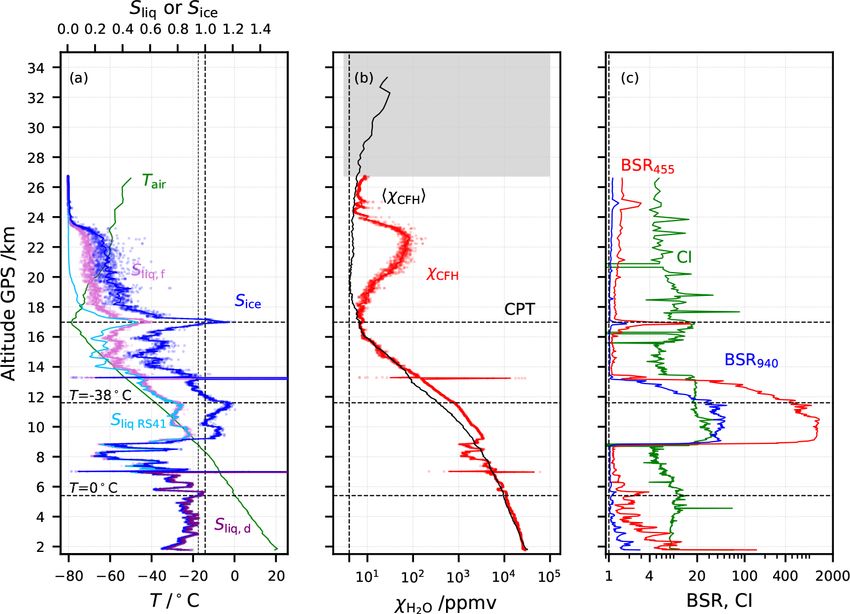
T. Jorge et al.: Understanding balloon-borne frost point hygrometer measurements                                                  245

                                                                        lower and an upper estimate of liquid water content (LWC);
                                                                        see Table 1. The lower estimate was constrained by the
                                                                        amount of ice required to sublimate in the stratosphere
                                                                        from the CFH intake tube in order to explain the observed
                                                                        contamination as determined by the computational fluid
                                                                        dynamics simulations discussed in the next sections. The
                                                                        upper estimate was determined such that it would provide
                                                                        the sum of the amount of ice sublimated in the stratosphere
                                                                        plus the amount sublimated in the upper troposphere, the
                                                                        latter computed from the difference between χRS41 and χCFH .
                                                                        These estimates are discussed more thoroughly in Sect. 5.2
                                                                        and 5.3.
                                                                           In Fig. 4, we see that both simulations for lower and upper
                                                                        estimates showed glaciation times of a smaller droplet mode
Figure 4. Modelling of the Wegener–Bergeron–Findeisen process           of τg ∼ 6 min and of the bigger droplet mode of τg ∼ 17 min.
in mixed-phase cloud demonstrating that flight NT011 likely             The overlap with the range of observed Sliq and Sice lasted
encountered supercooled liquid droplets. Solid lines: lower estimate
                                                                        for about 7 min, demonstrating that the cloud at 9.25–10 km
of liquid water content (LWC). Dashed lines: upper estimate
(see text). Initial size distributions for lower estimate simulation:
                                                                        in NT011 may have contained sufficient supercooled liquid
nice = 0.02 cm−3 , rice = 10 µm; nliq,1 = 10 cm−3 , rliq,1 = 10 µm;     to explain the contamination.
nliq,2 = 0.003 cm−3 , rliq,2 = 100 µm. Initial size distributions for
                                                                           Flights NT029 and NT007 showed very similar cold
upper estimate simulation are identical but with 50 % larger            mixed-phase clouds in terms of temperature, extent, and
nliq,1 and nliq,2 . (a) Blue lines: ice water content (IWC); purple     altitude to the mixed-phase cloud in NT011. These clouds
lines: LWC; (b) blue lines: ice saturation ratio (Sice ); purple        also fulfilled the water (Sliq > 0.85) and ice (Sice > 1.0)
lines: liquid water saturation ratio (Sliq ) for lower and upper        saturation and the COBALD CI (> 20) criteria of the
estimates. Glaciation times of small droplets τg,1 ∼ 6 min, of big      mixed-phase cloud of NT011. Flight NT007 also showed
droplets τg,2 ∼ 17 min. Shaded-saturated ratios: observed ranges        a warmer mixed-phase cloud at lower altitude. The results
from Fig. 3. Vertical arrows: time when smaller liquid droplets fully   of the simulation for flights NT029 and NT007 are shown
evaporated. The computed time interval with Sice and Sliq matching      in Figs. S3 and S11. Table 1 provides an overview of
flight observations is 1t ∼ 7 min.                                      supercooled or mixed-phase cloud appearances in the three
                                                                        analysed soundings.
                                                                           These simulations make a causal relationship between
   We modelled the Bergeron–Findeisen process in these                  the mixed-phase cloud and the CFH intake contamination
clouds by applying Eq. (1) to both the evaporating droplets             plausible. In addition, the updraft cores of cold clouds
(Sliq < 1) and the growing ice crystals (Sice > 1). We chose            observed by Lawson et al. (2017) over the Colorado
the size distribution of the liquid droplets to be bimodal in           and Wyoming high plains support these assumptions, as
order to approximate in situ observations of broad droplet              these clouds did not experience secondary ice formation
spectra in mixed-phase clouds (Korolev et al., 2017), with              and significant concentrations of supercooled liquid in the
small liquid droplets rliq,1 = 10 µm, nliq,1 = 10 cm−3 and              form of small drops have survived temperatures as low as
big liquid droplets rliq,2 = 100 µm, nliq,2 = 0.003 cm−3 . We           −37.5 ◦ C. Observed ice crystal number densities were lower
considered the number density of ice crystals to be consistent          than 4 cm−3 in clouds warmer than Tair = −23 ◦ C, increasing
with ice nucleation particles (INP) at about 0.02 cm−3                  to 77 cm−3 at Tair = −25 ◦ C and to several hundred per
(DeMott et al., 2010), neglecting secondary ice production              cm−3 at even lower temperatures. Thus, some of the clouds
processes, which might have enhanced ice number densities               described by Lawson et al. (2017) contained fewer ice
(Lawson et al., 2017) but would be highly uncertain. During             particles and more supercooled droplets than the example
the evolution of the mixed phase under the conditions                   treated here.
characteristic for the lower end of the cloud in NT011 (9.25–
10 km), the many small liquid droplets evaporated first,
providing favourable conditions for the fewer large droplets,           3   Balloon pendulum movement
which would have needed about 20 min to finally evaporate;
see Fig. 4.                                                             As we show below by means of computational fluid
   The low concentration of ice crystals and the bimodality             dynamics (CFD) simulations, the passage through clouds
of the liquid droplet distribution allowed the bigger                   containing supercooled water leads to hardly any collisions
droplets to exist for a relatively long period of time in a             of the droplets with the walls of the intake tube, if the
mildly subsaturated environment (Sliq ∼ 0.90–0.85). For the             airflow is parallel to the walls. Under those conditions,
simulation, we assumed two different initial distributions: a           only the mirror holder which is perpendicular to the airflow

https://doi.org/10.5194/amt-14-239-2021                                                     Atmos. Meas. Tech., 14, 239–268, 2021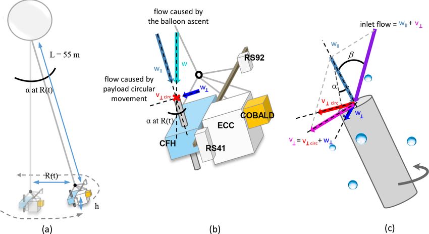
246 T. Jorge et al.: Understanding balloon-borne frost point hygrometer measurements
Table 1. Lower cloud edge, thickness of cloud fraction containing supercooled liquid droplets, and estimated liquid water content (LWC) in
mixed-phase clouds for flights NT007, NT011 and NT029.
Flights In cloud
Lower cloud edge (km) Thickness (m) LWC (g m−3 )
Lower estimate Upper estimate
NT007 6.25 and 9.2 750 + 600 0.080 + 0.020 0.137 + 0.034
NT011 9.25 750 0.011 0.016
NT029 8.1 1000 0.032 0.160
and extends into the intake tube causes collisions of larger in m s−1 . Figure 5c shows the residual payload motion
droplets. Below the mirror holder, a recirculation cell might relative to the balloon after “detrending”, i.e. subtracting the
also cause some of the smaller droplets to collide; however, average trajectory of the payload. We obtained the average
this would hardly affect the humidity measurement on the payload trajectory or balloon trajectory by smoothing the
mirror. The situation changes dramatically when the air payload trajectory with a moving average corresponding
enters the intake tube at a non-zero angle, as would happen to the pendulum oscillation period, which we evaluated
when pendulum oscillations and circular movement of the by two independent methods. First, we considered the
balloon payload induce a component of the payload motion ideal pendulum oscillation frequency, ω = (g/L)1/2 , where
perpendicular to the tube walls. Such pendulum oscillations L is the length of the pendulum, in our case 55 m and
and circular movement have been documented in the g = 9.81 m s−2 . This yielded the oscillation period τ =
literature (e.g. Kräuchi et al., 2016). Here, we approximated 2π/ω = 15 s. Second, we confirmed this result by means
the balloon plus payload by a two-body system connected of a fast Fourier transform (FFT) analysis on the latitude
by a weightless nylon cord and quantified the oscillations in and longitude detrended time series; see Appendix A. We
terms of the instantaneous displacement of the payload from concluded that, independently of the moving average used
the balloon path. We then used the displacement to calculate to detrend the longitude and latitude used in the FFT, the
the tilt of the payload relative to the flow and used the tilt oscillation period was τ ∼ 16.6 s. The same analysis was
angle and the associated horizontal velocity of the payload to done for the clouds in flights NT029 and NT007, and the
quantitatively estimate the internal icing of the intake tube. results are shown in Figs. S4 and S12.
Figure 5c also provides information on the degree to which
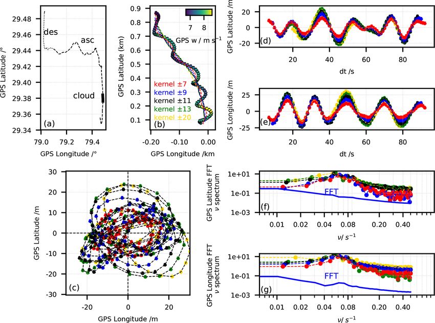
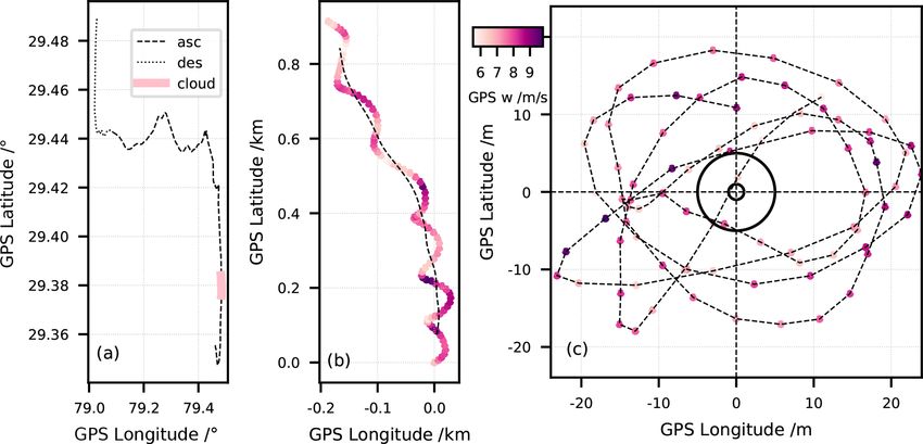
3.1 Pendulum oscillations derived from GPS data the balloon itself might contribute to the contamination.
The approximate balloon sizes at launch and burst are
We isolated the payload oscillations in relation to the balloon depicted as circles with 1 and 5 m radius, respectively. The
by removing the averaged trajectory of the payload. Figure 5a circular movement placed the payload typically far outside
shows the horizontally projected trajectory of NT011, the balloon wake, only sporadically penetrating the wake.
travelling first about 10 km northward in the troposphere The lack of periodic signs of contamination rendered it
and then about 40 km westward in the stratosphere before unlikely that H2 O collected by the balloon’s skin contributed
the balloon burst. The thick pink line shows the part of the to the observed contamination. However, this behaviour
trajectory, where the sonde flew through the cloud containing changed above ∼ 27 km altitude, where the H2 O partial
supercooled droplets, between 9.25 and 10 km altitude (see pressure became sufficiently low and the swing and circular
Fig. 3). The contamination happened most likely in this movement of the payload was also weaker, so that the
segment of the flight. balloon outgassing started to dominate over the natural
Figure 5b zooms in on this cloudy section1 , showing signal, leading to a systematic contamination in virtually
the 1 s GPS data colour-coded by the ascent velocity every sounding (see Sect. 5.4).
Figure 6a shows a schematic of the balloon and payload
1 The coordinates were transformed from degrees lat/long to
as a two-body system and illustrates the displacement of
distances in km using the geographical distance equation from the payload from under the balloon. From Fig. 5c we see
h i1/2
a spherical earth to a plane, d = Re (1φ)2 + (cos (φm ) 1λ)2 that the radial displacement R of the payload in relation to
(Wikipedia, 2018), where the bottom of the cloud (λ0 , φ0 ) was the balloon position for flight NT011 was typically larger
taken as the origin (0,0) of this new coordinate system. Differences than 5 m (only 4 % of the measurements have R < 5 m). The
in longitude and latitude were calculated in radians as 1λ(t) = corresponding tilt angle α is
λ(t) − λ0 and 1φ(t) = φ(t) − φ0 , respectively. Distances d were
given in km, Re is the Earth’s radius (6371 km), and the mean R(t)
latitude φm was taken as φ0 . α(t) = sin−1 > 5◦ . (2)
L
Atmos. Meas. Tech., 14, 239–268, 2021 https://doi.org/10.5194/amt-14-239-2021
T. Jorge et al.: Understanding balloon-borne frost point hygrometer measurements 247
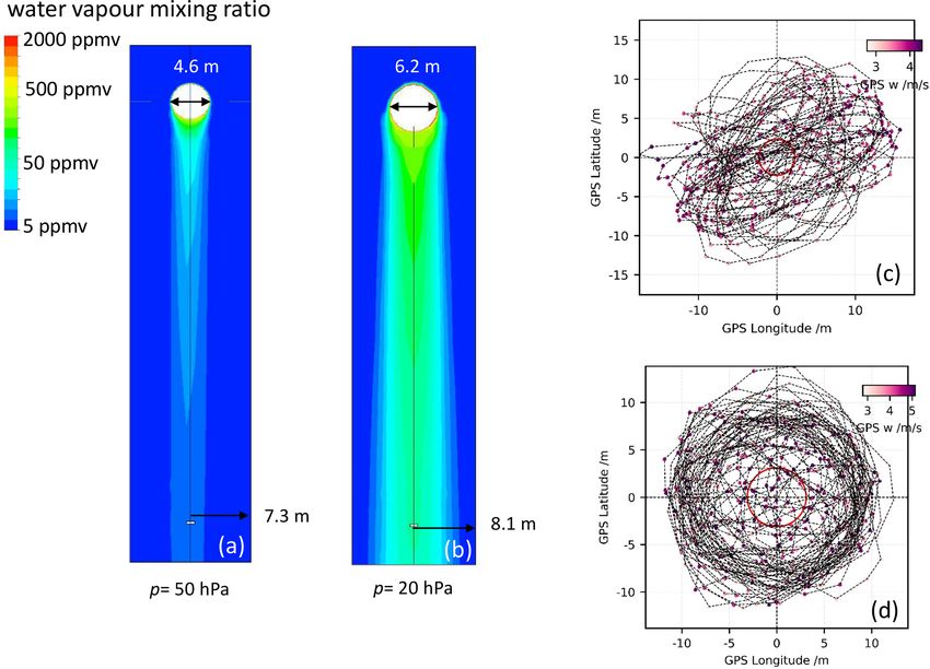
Figure 5. Pendulum analysis for the section of flight NT011 traversing the mixed-phase cloud. (a) Payload trajectory for the entire flight:
ascent (dashed), descent (dotted) and mixed-phase cloud between 9.25 and 10 km altitude (thick pink line). (b) Zoom-in on the mixed-
phase cloud with 1 s GPS data of payload trajectory (symbols) and derived balloon trajectory (dashed). (c) Detrended payload oscillations;
approximate balloon sizes on the ground (r = 1 m) and at burst (r = 5 m) are shown by two circles. Colour code in panels (b) and (c): balloon
ascent velocity.
Figure 6. (a) Schematic of balloon and payload (not to scale). Payload is connected to the balloon by a 55 m long lightweight nylon cord.
Payload oscillates with tilt angles α up to 25◦ during ascent. (b) Schematic of payload with the two radiosondes (RS41 and RS92) and the
three instruments (CFH, ECC Ozone and COBALD) and of intake flow geometry due to balloon ascent and payload circular movement. The
flow caused by the vertical balloon ascent (w) has a component parallel to the intake tube (w|| ) and a component perpendicular to the tube
walls (w⊥ ). Circular movement of the payload adds an additional component (v ⊥,circ ) in the plane perpendicular to the intake tube. (c) The
total velocity perpendicular to the tube becomes v ⊥ = v ⊥,circ + w⊥ . The total perpendicular velocity v ⊥ and the parallel component of the
ascent velocity to the intake tube w || determine the inlet flow and the impact angle β.
The maximum displacement was Rmax ∼ 23 m, corre- flight NT029 were of the same order of magnitude as the
sponding to a tilt angle αmax ∼ 25◦ . On average, hRi ∼ 15 m ones observed in the cloud of flight NT011, while for flight
and hαi ∼ 16◦ , which represented a significant deviation NT007 these were much smaller, almost half. We believe this
from a flow through the tube parallel to the tube walls. The difference stems from the different ascent velocities in the
tilt angles α of the payload in the mixed-phase cloud of three flights.
https://doi.org/10.5194/amt-14-239-2021 Atmos. Meas. Tech., 14, 239–268, 2021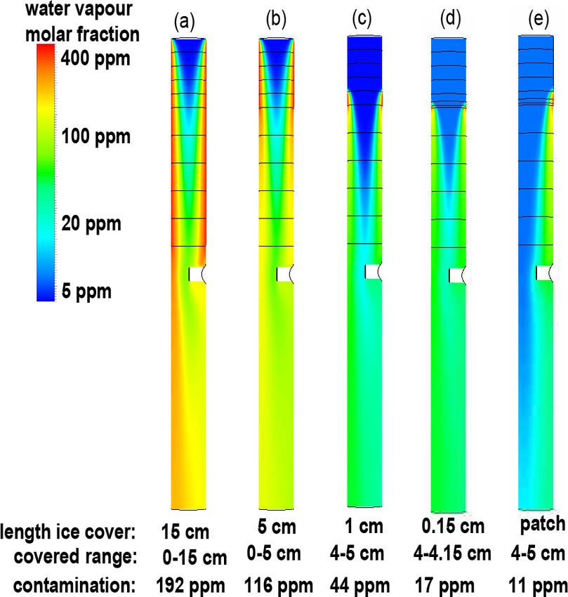
248                                      T. Jorge et al.: Understanding balloon-borne frost point hygrometer measurements

   Figure 6b shows how the flow through the CFH intake tube
can be separated into flow parallel to the tube (w || ) and flow
perpendicular to the tube (w⊥ ). Figure 6b also shows how
the different instruments are connected in the payload. The
impact angle (β) of droplets onto the CFH intake tube was
then partly determined by w ⊥ and w|| and consequently α.
Moreover, the associated horizontal circular movement led
to additional sideways impact, which we show to be even
more important.

3.2   Impact angles derived from payload motion

Impact of droplets on the walls of the intake tube was forced
by two effects that caused an airflow in the “horizontal
plane”, i.e. the plane whose normal was the tube axis:

  i. the tube was tilted relative to the ascent flow, leading to
     the velocity v ⊥,tilt = w ⊥ ;
                                                                      Figure 7. Probability density functions (pdfs) of impact parameters
 ii. the tube itself had a horizontal velocity v ⊥,circ caused        at the top end of the CFH intake tube during the passage through the
     by the swinging or circular movement of the payload.             mixed-phase cloud of flight NT011. (a) Velocity v⊥ perpendicular
                                                                      to the tube walls; (b) velocity w|| parallel to the axis of the tube;
   The vector sum of (i) and (ii) gave the total velocity             (c) impact angle (β).
perpendicular to the tube walls v ⊥ = v ⊥,tilt + v ⊥,circ ; refer
to Eq. (B4). Appendix B provides more details of the vector
relations. In addition, we took into account the possibility          calculated from the perpendicular velocities’ sum (v ⊥ ) and
of droplet impact on the mirror holder in the centre of the           the parallel component of the inlet flow (w|| ) as shown
tube, even when the flow was perfectly aligned to the tube,           in Fig. 6c. As the horizontal impact speed could be as
but compared to (i) and (ii) this was a smaller contribution          high as 10 m s−1 , this corresponded to a maximum impact
because larger droplets impacted already at the beginning             angle β = 53◦ . Such large impact angles are the reason why
of the tube and many of the smaller ones, which made it to            the CFH flying through mixed-phase clouds encounters a
the middle of the tube, were able to curve around the mirror          large risk of droplet collisions and freezing, accumulating
holder and avoid contact.                                             potentially thick ice layers inside the intake tube, which
   Figure 5c shows that the residual motion of the payload            renders further measurements in the stratosphere either
resembles a circular motion with radius R = 15 m. Here, we            impossible or possible only after a long recovery period of
only highlight the relevant magnitudes, but we provide a              the instrument (i.e. until the ice sublimates). As a result from
full treatment in Appendix B. The perpendicular velocity              the full numerical treatment of the impacts in Appendix B,
associated with the tube tilt (w⊥ = v⊥,tilt = w sin α) can be         Fig. 7 shows the probability density functions (pdfs) of
determined from the tilt angle α and the ascent velocity              the magnitude of the perpendicular velocity (v ⊥ ) to the
w ∼ 7.5 m s−1 (Fig. 3a). Equation (2) with R(t) = 15 m                intake tube walls and of the parallel component of the
and L = 55 m yields α = 16◦ and v⊥,tilt = 2.1 m s−1 . The             ascent velocity (w|| ) and the impact angle (β) as derived
perpendicular velocity associated with the payload circular           for the intake tube in the 9.25–10.0 km cloud section in
movement (v ⊥,circ ) can be calculated from the difference            flight NT011. Similar figures are shown for flights NT029
between consecutive measurements after detrending based               and NT007 in the Supplement. Perpendicular velocities were
on the GPS position received every second. Figure 5c shows            smaller for flight NT007 but, as the ascent velocity was also
that v⊥,circ can be as big as 10 m s−1 when the payload               smaller in this flight, the impact angles were equivalent to
traverses the equilibrium point, straight below the balloon,          those observed in flights NT011 and NT029.
or as small as 2 m s−1 far from the equilibrium point. The
circular movement of the payload leads to generally more
impacts than the tilt of the tube. Here, the radially directed tilt   4   Computational fluid dynamic simulations
contribution (2.1 m s−1 ) and the circular progression added
as the sum of orthogonal vectors increase the typical 5 m s−1         CFD tools have become commonly used in environmental
circular speed (see Fig. 5c) to only 5.4 m s−1 , i.e. less than       studies, e.g. for error estimation of lidar and sodar Doppler
10 %.                                                                 beam swinging measurements in wakes of wind turbines
   After accounting for the direction of movement when                (Lundquist et al., 2015), in new designs of photooxidation
combining tilt and circular movement, the impact angle was            flow tube reactors (Huang et al., 2017), or to improve

Atmos. Meas. Tech., 14, 239–268, 2021                                                     https://doi.org/10.5194/amt-14-239-2021
T. Jorge et al.: Understanding balloon-borne frost point hygrometer measurements 249
vehicle-based wind measurements (Hanlon and Risk, 2018). scheme changes from radial to Cartesian coordinates with a
Here, we used CFD to estimate collision efficiencies of liquid grid spacing of 1.5 mm.
droplets with different sizes encountering the CFH intake
tube under various impact angles in order to understand first 4.2 FLUENT computational fluid dynamics software
the ice build-up and second its sublimation from the icy
intake to the passing airflow. We used the academic version We used a 3D steady-state pressure-based solver. As
of FLUENT and ANSYS Workbench 14.5 Release (ANSYS, recommended for wall-affected flow with small Reynolds
2012). FLUENT is a fluid simulation software used to predict numbers, where turbulent resolution near the wall is
fluid flow, heat and mass transfer, chemical reactions and important, we used an SST (shear stress transport) k-ω model
other related phenomena. FLUENT has advanced physics (CFDWiki, 2011; ANSYS, 2012). The fluid material, air, was
modelling capabilities which include turbulence models, treated as a three-substance mixture of N2 , O2 and H2 O. We
multiphase flows, heat transfer, combustion, and others. specified how FLUENT computes the material properties,
Here, FLUENT is used for the first time to investigate the namely calculating density (ρ) using an incompressible ideal
operation of a balloon-borne instrument. For this study, the gas law:
only feature not available was the water vapour pressure pop
parameterization, which was added to the simulation through ρ= P mi , (4)
RT i Mi
a user-defined function. For our study, we make most use of
the ANSYS Workbench integrated approach from geometry where pop is the simulation-defined operating pressure in Pa,
to mesh to simulation to results visualization. R is the ideal gas constant, T is the absolute temperature, and
mi and Mi are the mass fraction and molar mass of species
4.1 Geometry and mesh i, respectively. Heat capacity (cp ) was calculated using a
FLUENT-defined mixing law:
By means of ANSYS Workbench, a mesh was developed X
mapping the intake tube geometry and providing the optimal cp = mi cp,i . (5)
geometric coverage. The CFH intake tube geometry was as i
described by Vömel et al. (2007c): a 2.5 cm diameter 34 cm
long cylinder. The walls of the intake tube have a thickness of In the dilute approximation scheme, the mass diffusion flux
25 µm but are approximated as infinitely thin. At the centre of of a chemical species in a mixture was calculated according
the tube, the mirror holder is mapped by a cylinder extending to Fick’s law:
1.25 cm from the wall, oriented perpendicular to the flow. ∂mi
The mirror holder is 7 mm in diameter. The mirror is the base Ji = ρDi , (6)
∂x
of the cylinder parallel to the flow at the centre of the tube.
The mesh is shown in Fig. 8. As a mesh assembly method where Di is the diffusion coefficient of species i in the
we used “cut cell”, which provides cuboid-shaped elements mixture. This relation is strictly valid when the mixture
aligned in the flow direction. Simulations had to cover composition stays approximately constant and the mass
conditions from the lower troposphere, where the liquid- fraction mi of a species is much smaller than 1. The
and mixed-phase clouds occurred, to the lower stratosphere amount of water expected in the simulations was less
where the sublimation of ice from the intake walls took place. than 1000 ppmv; therefore, the dilute approximation for the
This required coping with Reynolds numbers (Re) of the diffusion of water vapour in air, i = H2 O, was an accurate
order of 5000 in the cloud (i.e. turbulent flow inside the tube) description.
to 300 in the stratosphere (i.e. laminar flow) accompanied The temperature and pressure dependencies of the
by a transition around Re ∼ 2300 from turbulent to laminar diffusion coefficient of H2 O in air were given by Pruppacher
regimes: and Klett (1997)
cm2 T 1.96 p0
ρvL
Re = , (3) D = 0.211 , (7)
µ s T0 p
where ρ is the fluid’s density in kg m−3 (here of air), v is the where T0 = 273.15 K and p0 = 1013.25 hPa.
fluid’s velocity in m s−1 (relative to the intake tube), L is a For the viscosity and thermal conductivity, no mixture
characteristic linear dimension in m (here the tube diameter), laws were considered. The values of viscosity and thermal
and µ is the fluid’s dynamic viscosity in kg m−1 s−1 . We conductivity were derived from a linear fit to air viscosity and
were especially interested in the near-wall effects, since the thermal conductivity of dry air (EngineeringToolbox, 2005).
sublimation and the collision efficiency were evaluated near Air viscosity was µa (T ) = (0.0545 × (T /K) + 2.203) ×
the wall. To enhance the mesh description near the wall, the 10−6 in kg m−1 s−1 and air thermal conductivity was ka =
−5 −3
first layer thickness is 0.2 mm. The subsequent layers grow 8.06 × 10 × (T /K) + 2.02 × 10 in W m−1 K−1 , both for
in thickness at a rate of 1.2 for a total of five layers before the T ∈ (193, 300 K). According to kinetic gas theory, both
https://doi.org/10.5194/amt-14-239-2021 Atmos. Meas. Tech., 14, 239–268, 2021250 T. Jorge et al.: Understanding balloon-borne frost point hygrometer measurements
Figure 8. Cryogenic frost point hygrometer (CFH) intake tube mesh and geometry. The coordinate origin is located at the top centre of the
intake tube. (a, b) Detailed views of the mirror holder on the y = 0 and x = 0 planes. (c) Intake tube cross section. (d, e) Intake tube on the
y = 0 and x = 0 planes. Images used courtesy of ANSYS, Inc.
properties are only weakly pressure-dependent (neglected thus conserving mass flux. For our simulations, we took the
here). balloon ascent velocity as the velocity of the flow entering
Velocity-inlet and pressure-outlet boundary conditions the intake tube at the top plane.
were defined for the intake tube. For the velocity- The mirror holder slowed the flow upstream, created a
inlet boundary conditions, it was possible to define the recirculation region downstream, and accelerated the flow
velocity magnitude and direction, turbulence intensity, and in front of the mirror. The flow accelerated up to 150 % of
temperature. the fully developed flow velocity in the tube centre. In the
troposphere, the medium was denser and the flow was in the
4.2.1 Velocity and flow profiles turbulent regime. Turbulent flows develop faster into a fully
developed regime; see Fig. 9a–b.
Figure 9a–b show two examples of velocity profiles
computed by FLUENT for two pairs of pressures and 4.2.2 Discrete-phase model
temperatures as they occurred in NT011, p = 310 hPa and
T = −20 ◦ C and p = 33 hPa and T = −58.7 ◦ C. The two We used FLUENT’s discrete-phase module to compute the
examples were done for the same inlet velocity of 5 m s−1 . collision efficiency for water droplets entering the tube
In the lower-pressure case, the Reynolds number was low together with the air at some impact angle. The droplets were
and the flow was laminar. In the higher-pressure case the accelerated in the same direction as the airflow when they
Reynolds number was higher than 2300 and the flow was entered the tube and either managed to avoid a collision with
turbulent. As expected for the flow in a cylindrical tube, the the wall or hit it at some distance down the tube. We injected
flow velocity decreased towards the tube walls, became zero one particle through each of the cells at the top inlet plane
at the wall and in return accelerated at the centre of the tube, and repeated this procedure for droplets of different sizes.
Atmos. Meas. Tech., 14, 239–268, 2021 https://doi.org/10.5194/amt-14-239-2021T. Jorge et al.: Understanding balloon-borne frost point hygrometer measurements 251 Figure 9. (a, b) FLUENT simulation results for airflow velocity (centre cut through mirror holder). (a) p = 310 hPa and T = −20 ◦ C and (b) p = 33 hPa and T = −58.7 ◦ C simulations with inlet velocity 5 m s−1 normal to the inlet plane. (c) Collision efficiency analysis based on FLUENT simulation results for particle tracks of hydrometeors with radii between 10 and 500 µm (colour-coding). The figure shows the top 7 cm of the intake tube. Flow simulations are for the mixed-phase cloud of flight NT011, p = 310 hPa and T = −20 ◦ C. Inlet velocity is w || = 7.5 m s−1 parallel to the tube (largely due to the balloon’s ascent velocity) and v ⊥ = 6 m s−1 perpendicular to the tube wall (largely due to the swinging motion of the payload), which results in an impact angle β of about 39◦ . Images used courtesy of ANSYS, Inc. For each of the mixed-phase cloud simulations, we defined tube wall (see Fig. 8c). Therefore, we normalized all collision the droplet diameter, impact angle β and velocity magnitude. efficiency results to the top inlet plane cell surface density, At the top of the tube, the impact angles and velocities of the removing the effect of the mesh density from the results. The droplets were assumed to be identical to the airflow. collision efficiency results are provided in Figs. 11, S6, S14 The simulations in Fig. 9c were run with NT011 cloud and S15 for the different mixed-phase clouds considered. conditions, p = 310 hPa and T = −20 ◦ C. The velocity at the intake tube inlet surface was 7.5 m s−1 in the parallel 4.2.3 Species transport component (z direction) and 6 m s−1 in the perpendicular component (x direction), which corresponded to an impact The two key aspects controlling the level of contamination angle of about 39◦ . For clarity, Fig. 9c displays only one are the temperature of the ice layer and intake tube and the every sixth droplet trajectory. Only the first 7 cm of the length of the ice layer inside the intake tube. Warmer ice intake tube are shown. As expected, the airflow affected provides the incoming air with a higher content of water different size droplets differently. Smaller droplets had less vapour than colder ice. Simulations with longer ice layers inertia and hence tended to stay within the airflow, avoiding inside the intake tube present more severe contamination collisions with the tube’s wall, while bigger droplets (with than simulations with shorter ice layers at the same air higher inertia) could not follow the streamlines and collided temperature. with the walls. Most 10 µm radius droplets avoided collision, We simulated the sublimation of ice into the gas flow while only the droplets entering very close to the intake tube by assuming the cells adjacent to the icy wall to be wall collided. The bigger droplets to some extent also re- saturated with respect to ice (using the vapour pressure adjusted with the flow, but many of them collided within the parameterization of Murphy and Koop, 2005). The tube was first 5 cm of the intake tube. Above 70 µm droplet radius there assumed to have the same temperature as the airflow (Vömel was no dependence of the total collision efficiency on droplet et al., 2007b). In the UTLS, the intake tube might be slightly size due to their large inertia. warmer than ambient air due to radiative heating. However, In order to calculate the build-up of ice by impaction and we do not expect this difference to be bigger than a few considering how the injection of liquid droplets was set up in tenths of a Kelvin (Philipona et al., 2013). The tube wall was FLUENT, with one droplet per cell in the top inlet plane, we divided in ring sections and each was controlled separately had to account for the mesh cell surface density. As discussed to create the effect of a longer or shorter ice layer inside above, the cell surface density was higher closer to the intake the intake tube. FLUENT calculated the distribution of the https://doi.org/10.5194/amt-14-239-2021 Atmos. Meas. Tech., 14, 239–268, 2021
You can also read