Emission Monitoring Mobile Experiment (EMME): an overview and first results of the St. Petersburg megacity campaign 2019
←
→
Page content transcription
If your browser does not render page correctly, please read the page content below
Atmos. Meas. Tech., 14, 1047–1073, 2021
https://doi.org/10.5194/amt-14-1047-2021
© Author(s) 2021. This work is distributed under
the Creative Commons Attribution 4.0 License.

Emission Monitoring Mobile Experiment (EMME): an overview
and first results of the St. Petersburg megacity campaign 2019
Maria V. Makarova1 , Carlos Alberti2 , Dmitry V. Ionov1 , Frank Hase2 , Stefani C. Foka1 , Thomas Blumenstock2 ,
Thorsten Warneke3 , Yana A. Virolainen1 , Vladimir S. Kostsov1 , Matthias Frey4 , Anatoly V. Poberovskii1 ,
Yuri M. Timofeyev1 , Nina N. Paramonova6 , Kristina A. Volkova1 , Nikita A. Zaitsev1 , Egor Y. Biryukov1 ,
Sergey I. Osipov1 , Boris K. Makarov5 , Alexander V. Polyakov1 , Viktor M. Ivakhov6 , Hamud Kh. Imhasin1 , and
Eugene F. Mikhailov1
1 Department    of Atmospheric Physics, Faculty of Physics, St. Petersburg State University, St. Petersburg, Russia
2 Institute of Meteorology and Climate Research IMK-ASF, Karlsruhe Institute of Technology, Karlsruhe, Germany
3 Institute of Environmental Physics and Institute of Remote Sensing, University of Bremen, Bremen, Germany
4 National Institute for Environmental Studies, Tsukuba, Japan
5 Institute of Nuclear Power Engineering, Peter the Great St. Petersburg Polytechnic University, St. Petersburg, Russia
6 Voeikov Main Geophysical Observatory, St. Petersburg, Russia

Correspondence: Maria Makarova (m.makarova@spbu.ru), Frank Hase (frank.hase@kit.edu)
and Dmitry Ionov (d.ionov@spbu.ru)

Received: 13 March 2020 – Discussion started: 22 April 2020
Revised: 29 September 2020 – Accepted: 30 November 2020 – Published: 10 February 2021

Abstract. Global climate change is one of the most important      total column amount of CO2 , CH4 and CO at upwind and
scientific, societal and economic contemporary challenges.        downwind locations on opposite sides of the city. The NO2
Fundamental understanding of the major processes driving          tropospheric column amount was observed along a circu-
climate change is the key problem which is to be solved not       lar highway around the city by continuous mobile measure-
only on a global but also on a regional scale. The accuracy       ments of scattered solar visible radiation with an OceanOp-
of regional climate modelling depends on a number of fac-         tics HR4000 spectrometer using the differential optical ab-
tors. One of these factors is the adequate and comprehensive      sorption spectroscopy (DOAS) technique. Simultaneously,
information on the anthropogenic impact which is highest in       air samples were collected in air bags for subsequent labo-
industrial regions and areas with dense population – modern       ratory analysis. The air samples were taken at the locations
megacities. Megacities are not only “heat islands”, but also      of FTIR observations at the ground level and also at altitudes
significant sources of emissions of various substances into       of about 100 m when air bags were lifted by a kite (in case of
the atmosphere, including greenhouse and reactive gases. In       suitable landscape and favourable wind conditions). The en-
2019, the mobile experiment EMME (Emission Monitoring             tire campaign consisted of 11 mostly cloudless days of mea-
Mobile Experiment) was conducted within the St. Petersburg        surements in March–April 2019. Planning of measurements
agglomeration (Russia) aiming to estimate the emission in-        for each day included the determination of optimal location
tensity of greenhouse (CO2 , CH4 ) and reactive (CO, NOx )        for FTIR spectrometers based on weather forecasts, com-
gases for St. Petersburg, which is the largest northern megac-    bined with the numerical modelling of the pollution transport
ity. St. Petersburg State University (Russia), Karlsruhe In-      in the megacity area. The real-time corrections of the FTIR
stitute of Technology (Germany) and the University of Bre-        operation sites were performed depending on the actual evo-
men (Germany) jointly ran this experiment. The core instru-       lution of the megacity NOx plume as detected by the mo-
ments of the campaign were two portable Bruker EM27/SUN           bile DOAS observations. The estimates of the St. Petersburg
Fourier transform infrared (FTIR) spectrometers which were        emission intensities for the considered greenhouse and reac-
used for ground-based remote sensing measurements of the          tive gases were obtained by coupling a box model and the

Published by Copernicus Publications on behalf of the European Geosciences Union.
1048                                              M. V. Makarova et al.: Emission Monitoring Mobile Experiment (EMME)

results of the EMME observational campaign using the mass               The quantification of the gas fluxes from the sources lo-
balance approach. The CO2 emission flux for St. Petersburg          cated on the earth’s surface can be carried out using vari-
as an area source was estimated to be 89 ± 28 kt km−2 yr−1 ,        ous methods: “forward” and “inverse” modelling (Maksyu-
which is 2 times higher than the corresponding value in the         tov et al., 2013; Turner et al., 2015), the eddy covariance
EDGAR database. The experiment revealed the CH4 emis-               method (Helfter et al., 2011, 2014a), the mass balance ap-
sion flux of 135 ± 68 t km−2 yr−1 , which is about 1 order of       proach (Zimnoch et al., 2010; Strong et al., 2011; Hiller et al.,
magnitude greater than the value reported by the official in-       2014a) and a technique based on radon measurements (Lopez
ventories of St. Petersburg emissions (∼ 25 t km−2 yr−1 for         et al., 2015). Depending on the method, the spatial coverage
2017). At the same time, for the urban territory of St. Peters-     of investigated sources can vary from the local (for exam-
burg, both the EMME experiment and the official inventories         ple, in the case of eddy covariance) to the mesoscale and
for 2017 give similar results for the CO anthropogenic flux         the global scale (the assimilation of satellite data in atmo-
(251 ± 104 t km−2 yr−1 vs. 410 t km−2 yr−1 ) and for the NOx        spheric models). Each of these approaches has its own set
anthropogenic flux (66 ± 28 t km−2 yr−1 vs. 69 t km−2 yr−1 ).       of unique advantages and limitations depending on specific
                                                                    spatial and/or temporal scales. Therefore the efficacy and ac-
                                                                    curacy of many of these methods remain the subject of scien-
                                                                    tific debate (Cambaliza et al., 2014; Hiller et al., 2014a). Of-
                                                                    ten, combinations of these methods can yield reduced uncer-
1   Introduction                                                    tainty of target parameters; at the same time a combination
                                                                    of different techniques often requires special field campaigns
Global climate change is one of the most important scien-           and comprehensive analysis (Hiller et al., 2014a, b).
tific, societal and economic contemporary challenges. Fun-              Recently, several studies were performed with the goal
damental understanding of the major processes driving cli-          to estimate the emissions of industrial regions and cities
mate change is the key problem which is to be solved not            by means of ground-based mobile measurements of tropo-
only on a global but also on a regional scale (IPCC, 2013;          spheric gaseous composition using FTIR and differential op-
WMO Greenhouse Gas Bulletin, 2018). The accuracy of re-             tical absorption spectroscopy (DOAS) techniques. Hase et al.
gional climate modelling depends on a number of factors.            (2015) and Zhao et al. (2019) applied portable FTIR spec-
One of these factors is the adequate and comprehensive in-          trometers for detecting greenhouse gas emissions of the ma-
formation on the anthropogenic impact which is highest in           jor city Berlin. In these studies, five portable EM27/SUN
industrial regions and areas with dense population – modern         spectrometers were used for the accurate and precise obser-
agglomerations and megacities. Agglomerations and megaci-           vations of column-averaged abundances of CO2 and CH4
ties are not only “heat islands”, but also significant sources of   around the major city of Berlin. It has been demonstrated
emissions of various substances into the atmosphere, includ-        that the CO2 emissions of Berlin can be clearly identified in
ing greenhouse and reactive gases (Zinchenko et al., 2002;          the observations. Chen et al. (2016) developed and used dif-
Wunch et al., 2009; Ammoura et al., 2014; Hase et al., 2015;        ferential column methodology (downwind–upwind column
Turner et al., 2015; Viatte et al., 2017). Estimating emission      differences) for the evaluation of CH4 emissions from dairy
intensity for industrial areas and cities requires precise mea-     farms in the Chino area. Vogel et al. (2019) investigated
surements of gas composition in the troposphere with a high         the Paris megacity emissions of CO2 by coupling the COC-
horizontal resolution on a regional scale. Existing ground-         CON observations and atmospheric transport model frame-
based observational networks, in particular ESRL (ESRL,             work (CHIMERE-CAMS) simulations. Luther et al. (2019)
2019), ICOS (ICOS, 2020), NDACC (NDACC, 2019) and                   explored the feasibility of estimating CH4 emissions for in-
TCCON (TCCON, 2019), are mainly focused on detecting                dividual coal mine ventilation shafts and groups of shafts.
the background concentrations of greenhouse gases. Most             They measured column-averaged dry-air mole fractions of
of the observational stations are sparsely distributed and lo-      methane XCH4 using the Bruker EM27/SUN FTIR spec-
cated relatively far from industrial and highly populated ar-       trometer which was installed on a truck moving through the
eas. EM27/SUN portable Fourier transform infrared (FTIR)            CH4 plumes in the Upper Silesian Coal Basin, while driving
spectrometers (Gisi et al., 2012; Frey et al., 2015) are very       in stop-and-go patterns. De Foy et al. (2007), Mellqvist et al.
promising instruments for the detection and quantification          (2010), Johansson et al. (2014) and Kille et al. (2017) have
of the emissions of greenhouse gases from mesoscale area            applied mobile FTIR (Solar Occultation Flux technique) and
sources like cities or industrial areas (Hase et al., 2015; Chen    mobile DOAS techniques to large-scale flux measurements.
et al., 2016). The data provided by these instruments are less      Babenhauserheide et al. (2020) estimated CO2 emissions
affected by the vertical exchange processes than the data ob-       from Tokyo using the long-term statistical analysis of XCO2
tained from in situ measurements. Also, in contrast to current      amounts measured at the Tsukuba TCCON site located near
space-based sensors, the ground-based portable FTIR spec-           Tokyo.
trometer data are essentially unaffected by the aerosol burden          The motivation of the present study originated from the
transported by the pollution plume.                                 fact that the number of observational stations for greenhouse

Atmos. Meas. Tech., 14, 1047–1073, 2021                                              https://doi.org/10.5194/amt-14-1047-2021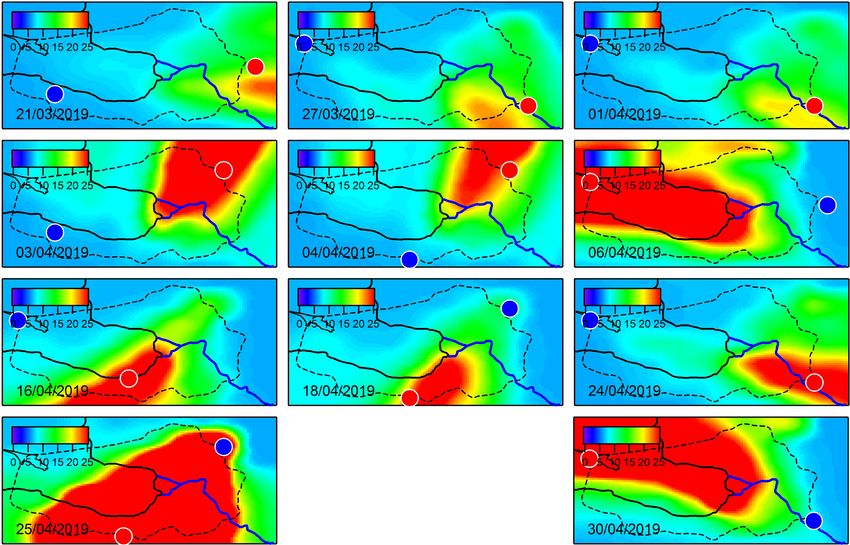
M. V. Makarova et al.: Emission Monitoring Mobile Experiment (EMME)                                                                1049

gas monitoring in the territory of Russia is very limited, and
there are considerable uncertainties of the greenhouse gas
flux estimations for the natural and anthropogenic sources
in Russia. St. Petersburg is the second largest megacity in
Russia, with a population of 5 million, and, in addition, it is
the northernmost city in the world with a population of over
1 million people. The goal of the present study was to esti-
mate the emissions of greenhouse (CO2 , CH4 ) and reactive
(CO, NOx ) gases from St. Petersburg by means of mobile
remote sensing techniques and direct in situ measurements.
The study was based on the observational campaign EMME-
2019 (Emission Monitoring Mobile Experiment) which was
performed in March–April 2019 in the territory of the St. Pe-
tersburg agglomeration. St. Petersburg State University (Rus-
sia), Karlsruhe Institute of Technology (Germany) and the
University of Bremen (Germany) jointly ran this experiment
in the frame of the international project VERIFY (VER-
                                                                    Figure 1. Illustration of the concept of EMME: two FTIR spectrom-
IFY, 2019). The idea and the methodology of EMME were
                                                                    eters at the upwind and downwind locations on opposite sides of the
based mainly on the studies by Hase et al. (2015), Ionov            city (no. 1 and no. 2, red and blue dots) and circular moving DOAS
and Poberovskii (2015), Chen et al. (2016) and Viatte et al.        technique spectrometer (no. 3). Ground-level air samples were col-
(2017).                                                             lected at locations no. 2 and no. 3. Collecting air portions with the
                                                                    help of a kite was done usually at the downwind location under
                                                                    suitable weather and landscape conditions. Pictogram png images:
2   Concept of EMME, instruments and the experiment                 https://www.cleanpng.com/, last access: 6 November 2019.
    planning

The concept of EMME is based on remote measurements of              frared solar radiation. The FTIR spectrometers are trans-
the total column amount of CO2 , CH4 and CO from two mo-            ported by cars to the measurement locations where they are
bile platforms located inside and outside the city plume (usu-      unloaded and installed outside. The geographic coordinates
ally at upwind and downwind locations on opposite sides of          are recorded by the GNSS (Global Navigation Satellite Sys-
the city of St. Petersburg) combined with the mobile circu-         tem) sensor. A detached car battery with an inverter is used
lar measurements of the tropospheric column amount of NO2           as a power supply which ensures about 3 h operation time.
from the third mobile platform moving in a non-stop mode;           Under cold weather conditions, the instruments are covered
the latter measurements are used for the real-time control of       by electric heating blankets. The integration time for a single
the megacity plume evolution. The simplified illustration of        spectrum constitutes about 1 min. Within this period, about
the concept is given in Fig. 1. The experiment requires clear-      10 interferograms are recorded and averaged, and then the
sky conditions since the instruments for remote sensing mea-        corresponding spectrum is recorded.
sure direct and scattered solar radiation. The ancillary mea-          The tropospheric NO2 column is derived from measure-
surements include control of the meteorological parameters          ments of the scattered solar radiation in the zenith direc-
and sampling of air portions at locations inside and outside        tion by the portable OceanOptics HR4000 automatic spec-
the city plume for subsequent laboratory analysis of concen-        trometer. This spectrometer is mounted on board a car and
trations of target gases. In order to assess the intensity of gas   connected to a portable computer to ensure uninterruptible
emissions by St. Petersburg, the mass balance approach is           recording of spectra. Measurements are fully automatic while
applied to the measurement data. The principal feature of           the car is moving. The location of the car is controlled by the
EMME is its integrated character: several different instru-         GNSS sensor and is routinely recorded by the onboard com-
ments are used, and, additionally, the planning of the field        puter for instant referencing of the results of measurements
experiment and data processing are performed with the help          to the car route. The sampling period of time (time of expo-
of numerical modelling of the transport of the megacity pol-        sure) for a single spectrum is calculated by the software tool
lution plume.                                                       accounting for illumination conditions and constitutes about
   The core instruments of the campaign are two portable            60 ms on average for the observations at about noon. Record-
Bruker EM27/SUN FTIR spectrometers (Gisi et al., 2012;              ing of spectra is done every 1 min; all single spectra obtained
Frey et al., 2015, Hase et al., 2016) which are used for            within this period are co-added. Thus, each final measure-
ground-based remote sensing measurements of the total col-          ment is the mean of about 1000 instant spectra. The route
umn amount of CO2 , CH4 and CO. The EM27/SUN in-                    includes the entire city ringway (the highway around St. Pe-
strument has a sun-tracking system and records direct in-           tersburg); therefore the main emission sources are inside the

https://doi.org/10.5194/amt-14-1047-2021                                               Atmos. Meas. Tech., 14, 1047–1073, 2021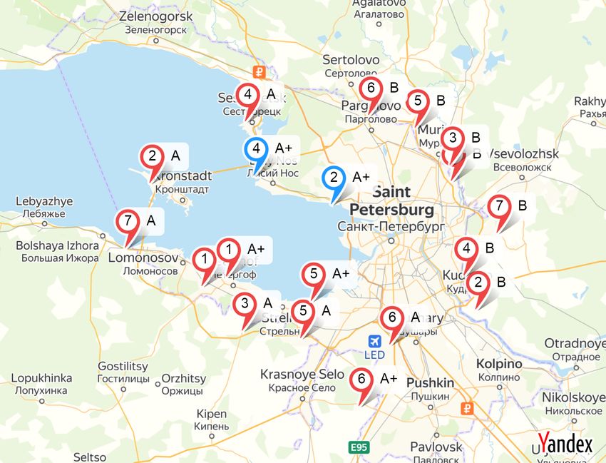
1050 M. V. Makarova et al.: Emission Monitoring Mobile Experiment (EMME)
route, and the position of the megacity plume can be detected tion. This information is critical for understanding whether it
with high accuracy. The described approach and the DOAS is possible to reach the desired up- and downwind locations
mobile experiment specific design have been implemented in proper time by different crews and to start simultaneous
previously in St. Petersburg, and the results have been pub- FTIR measurements.
lished by Ionov and Poberovskii (2012, 2015, 2017, 2019). Special attention was paid to the planning of the experi-
Air samples were collected at the locations of both FTIR ment a day before. We analysed the weather forecasts pre-
spectrometers in two air bags: when FTIR measurements sented by different sources with special attention to cloud
started (the first bag) and before completion of FTIR mea- cover and wind direction. Mainly, we used the cloud maps
surements (the second bag). Each bag was a 25 L Tedlar bag, from https://www.msn.com (last access: 12 November 2019).
sampled for about 40 min. In case of suitable weather and In order to determine FTIR measurement locations for a spe-
landscape conditions at the location of one of the FTIR spec- cific day, we made a forecast of the megacity plume us-
trometers, sampling bags were lifted by a kite to an altitude ing the HYSPLIT (HYbrid Single-Particle Lagrangian Inte-
of about 100 m. The laboratory analysis of the air samples grated Trajectories) model (Draxler and Hess, 1998; Stein
was performed with the help of gas analysers. A Los Gatos et al., 2015). In addition, in the morning of a measurement
Research GGA 24r-EP gas analyser was used for measuring day we monitored the cloud cover using web cameras which
the volume mixing ratio (vmr) of CH4 , CO2 and H2 O. A Los operated nearby the planned measurement locations.
Gatos Research CO 23r gas analyser was used for measur-
ing the vmr of CO and H2 O. The concentration of NO and
NO2 (NOx ) was measured by a ThermoScientific 42i-TL gas 3 Overview of the 2019 campaign
analyser.
For the monitoring of meteorological parameters, two The EMME field campaign in 2019 consisted of 11 d of
weather stations and the microwave radiometer RPG- measurements in March–April. Table A1 (see Appendix A)
HATPRO were used. One portable weather station was op- presents daily information on the location of FTIR spectrom-
erating either at upwind or at the downwind location of eters during the campaign, the FTIR spectrometer identifier,
FTIR spectrometers. The atmospheric pressure measure- number of bags of air samples, flight of a kite and air sam-
ments were performed at both up- and downwind locations. pling altitude. Below, we refer to the two Fourier Transform
The second stationary weather station was operating on the spectrometers (FTSs) as FTS no. 80 and FTS no. 84. In Ta-
roof of the building (56 m a.s.l.) of the Institute of Physics of ble A2 (please see Appendix A) we collect the main char-
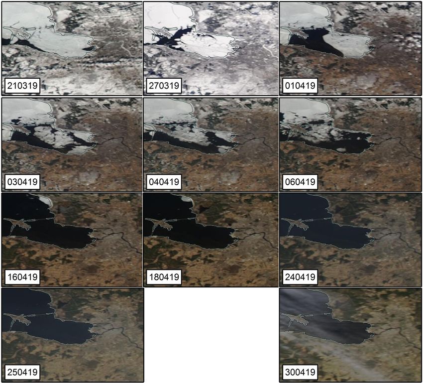
St. Petersburg State University (SPbU), located about 25 km acteristics of weather conditions for each measurement day.
west from the city centre. The RPG-HATPRO radiometer The satellite images of cloud cover detected by the MODIS
was operating also on the roof of this building and delivered satellite instrument in the vicinity of St. Petersburg are pre-
information on the temperature and humidity vertical profiles sented in Fig. A1 (see Appendix A). They confirm daytime
together with the information on the cloud liquid water path clear-sky conditions for the duration of the campaign, except
(Kostsov, 2015; Kostsov et al., 2018). the day of 30 April, when altocumulus translucidus clouds
The essential part of EMME was the preparatory stage started to develop.
which lasted for 3 months before the start of the campaign. During EMME-2019 we implemented two types of field
During this stage the optimal set of FTIR measurement lo- experiment setup regarding the position of FTIR spectrome-
cations in the close vicinity of the St. Petersburg ringway ters relative to the dominant air flow (wind) direction:
was determined accounting for several criteria. First, this set
– For most of the days of observations (10 of the 11),
of locations should have had sufficient spatial density to en-
FTIR spectrometers were installed along the wind di-
sure the possibility to perform up- and downwind FTIR mea-
rection line – in up- and downwind locations on oppo-
surements for practically any wind direction. Second, ev-
site sides of the city of St. Petersburg (Fig. 1, locations
ery location should have been convenient for car parking in
no. 1 and no. 2).
the ringway proximity and for the installation of the instru-
ments. We tried to choose the locations at a certain distance – For 16 April, the cross-sectional setup was imple-
from the highway and roads with intensive traffic in order to mented. FTIR spectrometers were located on the line
avoid contamination of air by local sources. The set of FTIR which is nearly perpendicular to the dominant wind di-
measurement locations around the St. Petersburg agglomera- rection line (not shown in Fig. 1).
tion which was chosen during the preparatory stage is shown
in Fig. 2. It should be emphasised that during the prepara- In order to forecast the spatial distribution of urban air pol-
tory stage a kind of rehearsal was carried out. This rehearsal lution on each day of campaign observations, we used the
has helped to reveal how time-consuming the following pro- HYSPLIT model. Following our previous experience of sim-
cesses are: loading the equipment on cars at the Institute of ulating the dispersion of urban contamination from St. Pe-
Physics, unloading the equipment at a measurement location tersburg, the NO2 content in the lower troposphere was set
and setting up and tuning the instruments for data acquisi- as a tracer of the polluted air mass distribution (Ionov and
Atmos. Meas. Tech., 14, 1047–1073, 2021 https://doi.org/10.5194/amt-14-1047-2021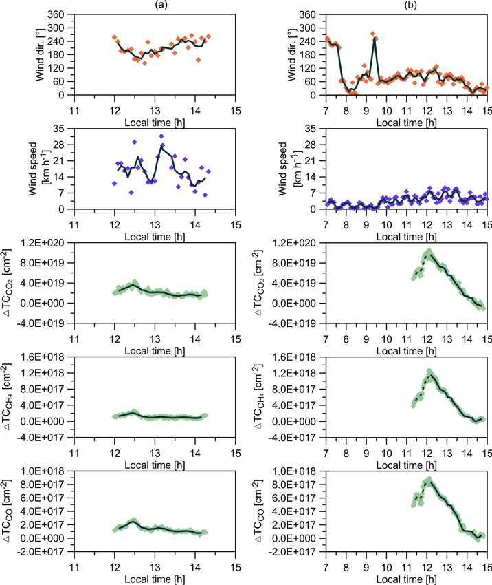
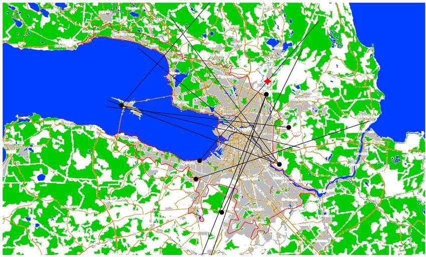
M. V. Makarova et al.: Emission Monitoring Mobile Experiment (EMME)                                                                    1051

Figure 2. The set of FTS locations around the St. Petersburg agglomeration. Locations are marked by letters “A” and “B” with numbers.
The “plus” sign near a location mark denotes that there is a possibility to use a local power supply at this location. The red colour denotes
primary locations, and the blue colour denotes secondary locations. Map data © 2019 Yandex.

Poberovskii, 2019). This numerical modelling was done by                 13:00 LT on each day of campaign observations, are pre-
means of the dispersion module within the offline version                sented in Fig. 3. The colour scale represents the spatial dis-
of HYSPLIT. It allowed the 3-D simulation of the genera-                 tribution of the NO2 column amount integrated within the
tion and dispersion of the NO2 plume to be performed from                boundary layer (∼ 1500 m). An animated version of such a
a set of given sources of anthropogenic NOx emission. The                forecast, showing the plume evolution, was generated and
model was configured in the same way as in our early stud-               shared among the campaign staff ∼ 12 h before each day of
ies (Ionov and Poberovskii, 2012, 2015, 2017). Similar to the            planned observations (an example of the animated forecast
most recent study by Ionov and Poberovskii (2019), the NOx               for 6 April 2019 is available at https://youtu.be/rgtq6JLPhig,
emissions were specified according to the official municipal             last access: 2 March 2020).
inventory of emission sources. The HYSPLIT grid domain                      Based on the plume evolution forecasts, the optimal pair
was set with the centre at 58.20◦ N and 30.75◦ E, the grid               of the FTIR spectrometer locations for the upcoming day of
spacing (horizontal spatial resolution) of 0.05◦ latitude and            measurements was chosen. This approach to the planning of
longitude and the grid span of 6.8◦ latitude and 14.1◦ lon-              the city campaign was implemented during 11 d of EMME-
gitude. The vertical grid consisted of 10 levels with the tops           2019, and the necessity to change the location of the FTIR
at 1, 25, 50, 100, 150, 250, 350, 500, 1000 and 1500 m. The              spectrometers occurred only once, on 18 April. For this day,
forecast meteorology data (vertical distributions of the hori-           the real-time information on the NO2 tropospheric column
zontal and vertical wind components, temperature and pres-               (TrC) acquired along the ring road by crew no. 3 using mo-
sure, etc.) were taken from the National Centers for Environ-            bile DOAS observations showed that the actual location of
mental Prediction Global Forecast System (NCEP GFS; ftp:                 the most polluted city plume area was different from one
//arlftp.arlhq.noaa.gov/forecast, last access: 2 March 2020)             which had been predicted by the HYSPLIT simulations. It
on the 1◦ × 1◦ latitude × longitude spatial grid. The maps               should be noted that the mobile DOAS observations were
of the NO2 plume, simulated by the HYSPLIT model for                     organised in such a way that the data on the TrC of NO2 for

https://doi.org/10.5194/amt-14-1047-2021                                                    Atmos. Meas. Tech., 14, 1047–1073, 2021
1052                                              M. V. Makarova et al.: Emission Monitoring Mobile Experiment (EMME)

Figure 3. The HYSPLIT model output for each of the campaign days (10:00 UTC) used as the forecast of the megacity plume while planning
the field campaign. The colour bar units for TCNO2 are [0–25] 1015 cm−2 . The blue line in the southeast indicates the river Neva.

the location outside the city plume were collected first. There      (the main interfering gases are H2 O, HDO, CH4 ), 4210–
were 2 d of FTIR measurements without mobile DOAS ob-                4320 cm−1 (the main interfering gases are H2 O, HDO, CH4 ),
servations due to technical issues. Our experience has shown         8353–8463 cm−1 and 5897–6145 cm−1 (the main interfering
that the HYSPLIT forecast was precise enough to ensure               gases are H2 O, HDO, CO2 ). The EM27/SUN spectrometer
proper selection of FTIR locations on these days.                    has a low spectral resolution of 0.5 cm−1 . Therefore the TCs
                                                                     are derived from the FTIR spectra through scaling of the a
                                                                     priori profiles of target gases (Frey et al., 2019). The required
4     Methods and algorithms of the experimental data                auxiliary data are the local ground pressure, the temperature
      processing                                                     profile and the a priori mixing ratio profiles of the gases. For
                                                                     ensuring consistency with the TCCON reference network in
4.1    FTIR and DOAS data processing
                                                                     this regard, these atmospheric profiles were provided by TC-
                                                                     CON. The ratio of the target gas TC to the retrieved O2 TC,
The dual-channel EM27/SUN spectrometer can measure to-
                                                                     which is suggested to be known and constant, gives us the
tal column abundances (TCs) of O2 , H2 O, CO2 , CH4 and
                                                                     column-averaged dry-air mole fraction (Xgas ) of the target
CO (Gisi et al., 2012; Hase et al., 2016). The processing
                                                                     gas (Wunch et al., 2011; Frey et al., 2015):
of the raw FTIR data (generation of spectra from raw inter-
ferograms and trace gas retrievals) is performed using the
software tools provided by the COCCON (Frey et al., 2019;                            TCgas    TCgas
                                                                     Xgas = 0.2095         =           ,                          (1)
COCCON, 2019). The required software is open-source and                              TCO2    TCdry air
freely available; the development of these tools has been sup-
ported by ESA. The interferograms recorded with FTS no. 80           where Xgas is the column-averaged dry-air mole fraction
and FTS no. 84 were the main input data. In the first process-       of the target gas (unit: dimensionless quantity), TCgas is
ing step, spectra are generated from the recorded DC-coupled         the total column of the target gas (unit: molec. m−2 ), TCO2
interferograms, including a DC correction (Keppel-Aleks              is the total column of O2 (unit: molec. m−2 ) and TCdry air
et al., 2007) and quality filtering. In the second processing        is the dry-air total column (unit: molec. m−2 ). Using Xgas
step, TCs of the target species are derived from the spec-           helps to reduce the effect of various possible systematic er-
tra. For the retrievals of the total columns of O2 , CO2 , CO,       rors (Wunch et al., 2011). To provide the compatibility of
H2 O and CH4 , the spectral regions recommended by Frey              EM27/SUN measurements with the WMO scale, and for
et al. (2019) and Hase et al. (2016) were taken. We present          consistency reasons, the retrieval software used for process-
these intervals in the respective order: 7765–8005 cm−1 (the         ing the EM27/SUN spectra also performs post-processing
main interfering gases are H2 O, HF, CO2 ), 6173–6390 cm−1           (Frey et al., 2015). Finally, we had both the TCgas and Xgas

Atmos. Meas. Tech., 14, 1047–1073, 2021                                                https://doi.org/10.5194/amt-14-1047-2021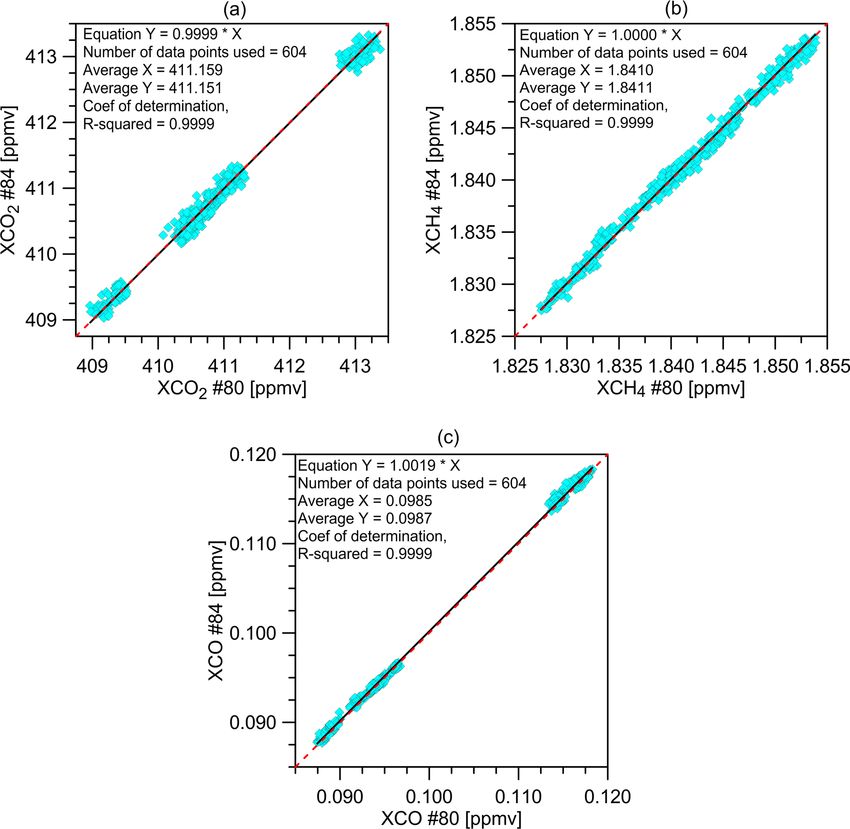
M. V. Makarova et al.: Emission Monitoring Mobile Experiment (EMME) 1053
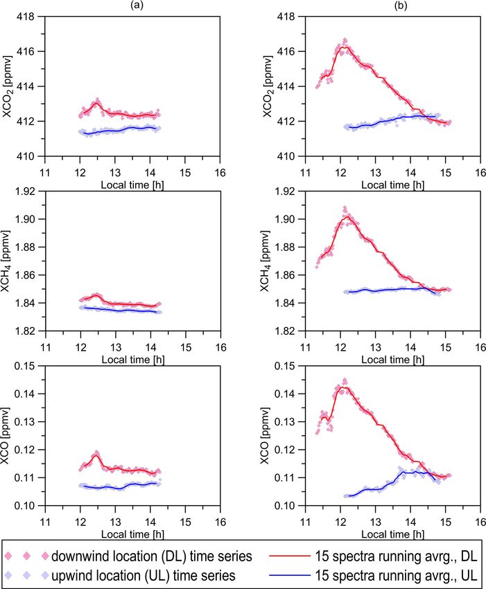
for each day of measurements at each observational location The scaled results of the side-by-side measurements of
at our disposal. XCO2 , XCH4 and XCO by FTS no. 80 and FTS no. 84 on
For the interpretation of spectral UV–Vis measurements 12 April 2019 at the St. Petersburg observational site are pre-
and the derivation of tropospheric NO2 content, the well sented in Fig. 5. The individual results and 15 min running
known DOAS method is used (Platt and Stutz, 2008). Ba- average data are shown. We used the side-by-side measure-
sically, the DOAS algorithm derives the NO2 atmospheric ments for estimating the optimal averaging period for the
content by fitting a reference NO2 absorption cross-section Xgas data. Averaging is the necessary prerequisite for using
to the measured zenith scattered radiance. The effective or these data for the evaluation of emission and for comparison
slant column density (SCD) of NO2 is retrieved in the 425– with the results of modelling. It should be emphasised that
485 nm fitting window. SCD is converted then to vertical col- the data sampling for other input parameters varies consid-
umn density (VCD) by means of a so-called air mass fac- erably. In order that all datasets are consistent, the optimal
tor, AMF (VCD = SCD/AMF), precalculated with a radia- sampling intervals were determined. For the FTIR measure-
tive transfer model (RTM). The spatio-temporal variations ments, the averaging interval has been selected in such a way
of stratospheric NO2 are negligible compared to these in a that short-term variations of measured quantities can be de-
polluted troposphere. Consequently, the variations of NO2 tected. As an example, we point to three local maxima of
vertical column observed in the data of our mobile DOAS XCH4 and XCO during the time period of 13:00–15:00. One
measurements are related to NO2 pollution in the boundary can see that these maxima with a half width of about 15–
layer (below ∼ 1.5 km). In general, such observations have 20 min and with amplitudes of ∼ 0.5 ppbv and of 0.1 ppbv
been proved to be an efficient technique to derive the an- for XCH4 and XCO, respectively, are nicely covered as well
thropogenic NOx flux in many studies worldwide (see, for as the increase of the greenhouse gases around noon, so the
example, Johansson et al., 2008, 2009; Rivera et al., 2009, chosen value of an averaging interval of 15 min seems rea-
2010; Ibrahim et al., 2010; Shaiganfar et al., 2011, 2015, sonable. The chosen averaging interval of 15 min is in good
2017; Wang et al., 2012; Wu et al., 2017). agreement with the estimation of the optimal integration time
(10 min) obtained as a result of the Allan analysis imple-
mented by Chen et al. (2016). Chen et al. (2016) applied
4.2 Side-by-side calibration of FTIR spectrometers
this approach for the differential measurements of XCO2 and
XCH4 performed by three EM27/SUN spectrometers within
The target quantity of our observations is the small differ- urban areas.
ence between two large values that are measured by differ-
ent instruments of the same type. Therefore, a careful cross- 4.3 Mass balance approach for area flux estimation
calibration of the instruments is of primary importance for
the considered experiment. Side-by-side calibrations of FTS The estimation of the area fluxes F was obtained on the ba-
no. 80 and FTS no. 84 were carried out on 12 April, 26 April, sis of a mass balance approach implemented in the form of
15 May and 16 May 2019. The instruments were installed a one-box model. Box models are a widely used technique
at the observational site of St. Petersburg State University for the evaluation of urban and other emission fluxes (Hanna
in Peterhof and operated simultaneously for the time pe- et al., 1982; Reid and Steyn, 1997; Arya, 1999; Zinchenko
riod of clear-sky weather, which lasted from half an hour et al., 2002; Zimnoch et al., 2010; Strong et al., 2011; Hiller
to several hours. The total number of spectra acquired dur- et al., 2014a; Chen et al., 2016; Makarova et al., 2018). In
ing cross-calibrations was 604. They were collected during our case the following equation for the calculation of area
about 10 h of simultaneous measurements. The scatter plots flux was used:
showing cross-comparison of the data are given in Fig. 4.
For all considered gases (CO2 , CH4 , CO), the results for 1TC (ti ) · Vj (ti )
Fj (ti ) = · k, (2)
column-averaged dry-air mole fractions (Xgas ) delivered by Lj (ti )
the two FTSs are in a very good agreement. The determi-
nation coefficients for CO2 , CH4 and CO are 0.9999(99), where F (unit: t km−2 yr−1 ) is the area flux, and ti denotes
0.9999(99) and 0.9999(89), respectively. The calibration fac- the day of a single field experiment in the frame of the ob-
tors obtained as a result of the side-by-side comparison were servational campaign. It should be emphasised that we used
used to convert XCO2 , XCH4 and XCO measured by spec- the steady-state approximation for all processes involved
trometer no. 80 to the scale of spectrometer no. 84. The re- within the duration of a single field experiment, so 1TC (unit:
sults of cross-calibration help to avoid an additional source molec. m−2 ) is the mean TC difference between downwind
of systematic error in the estimation of area fluxes. The root (TCd ) and upwind (TCu ) observations 1TC = TCd − TCu ,
mean square (rms) differences between time series of simul- V (unit: m s−1 ) is the mean wind speed and L (unit: m)
taneous measurements by FTS no. 80 and FTS no. 84 are is the mean length of a path of an air parcel which goes
equal to 0.10 ppm (0.025 %) for CO2 , 0.59 ppb (0.032 %) for through the urban territory of St. Petersburg agglomeration.
CH4 and 0.38 ppb (0.38 %) for CO. The k coefficient converts the value of area flux from units of
https://doi.org/10.5194/amt-14-1047-2021 Atmos. Meas. Tech., 14, 1047–1073, 2021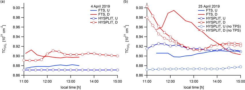
1054                                                M. V. Makarova et al.: Emission Monitoring Mobile Experiment (EMME)

Figure 4. The scatter plots of cross-comparison of the average mole fraction data during side-by-side calibrations.

molec. m−2 s−1 to units of t km−2 yr−1 :                                 the main contributor to the total error of NOx emission by the
                                                                         megacity of St. Petersburg, estimated from circular DOAS
      mgas · 31 536 × 106                                                measurements. It was also found that the direction of the
k=                        ,                                     (3)
               NA                                                        surface wind acquired by ground-based meteorological ob-
                                                                         servations often does not match the results of modelling of
where mgas is the molecular mass of the target gas (unit:                the pollution plume and the results of the NO2 mobile mea-
kg mol−1 ), NA is the Avogadro constant (unit: mol−1 ) and               surements (Ionov and Poberovskii, 2017). Apparently, the
31536 × 106 is the coefficient that converts the value of area           routine wind observations in the city are subject to significant
flux from units of kg m−2 s−1 to units of t km−2 yr−1 . The              local perturbations due to unavoidable interactions of the
data for the wind speed and the wind direction were taken                wind flow and the adjacent city buildings. It should be em-
from different sources of meteorological information (see                phasised that the HYSPLIT simulations of the fields of tro-
Sect. 4.3), and these sources are identified as j in Eq. (2).            pospheric NO2 demonstrate reasonable agreement with the
So, as a result, we obtained the set of values of F (t) for              plume dispersion observed by the circular mobile observa-
each of the meteorological data sources and for each day of              tions (Ionov and Poberovskii, 2017, 2019). The latter is also
field measurements. We note that below we will use the units             true for plume simulations, presented in the current study in
t km−2 yr−1 for the values of F (t).                                     Fig. 3. However, one can easily notice inconsistencies be-
                                                                         tween the dominant directions of plume movement and the
4.4    Wind field data                                                   surface winds as specified in Table A2 (see Appendix A):
                                                                         e.g. on 21 and 27 March and 1 and 24 April, when the city
Obviously, reliable wind field information is an important
                                                                         plume was moving towards southeast but the surface wind
prerequisite to get an accurate estimate of the target emis-
                                                                         was west-southwest (see Fig. 3). In order to get more accu-
sions from the data of remote spectroscopic measurements.
                                                                         rate wind information, we have considered additional sources
For instance, it has been noted by Ionov and Poberovskii
                                                                         of wind data:
(2015) that the uncertainty of the surface wind direction is

Atmos. Meas. Tech., 14, 1047–1073, 2021                                                    https://doi.org/10.5194/amt-14-1047-2021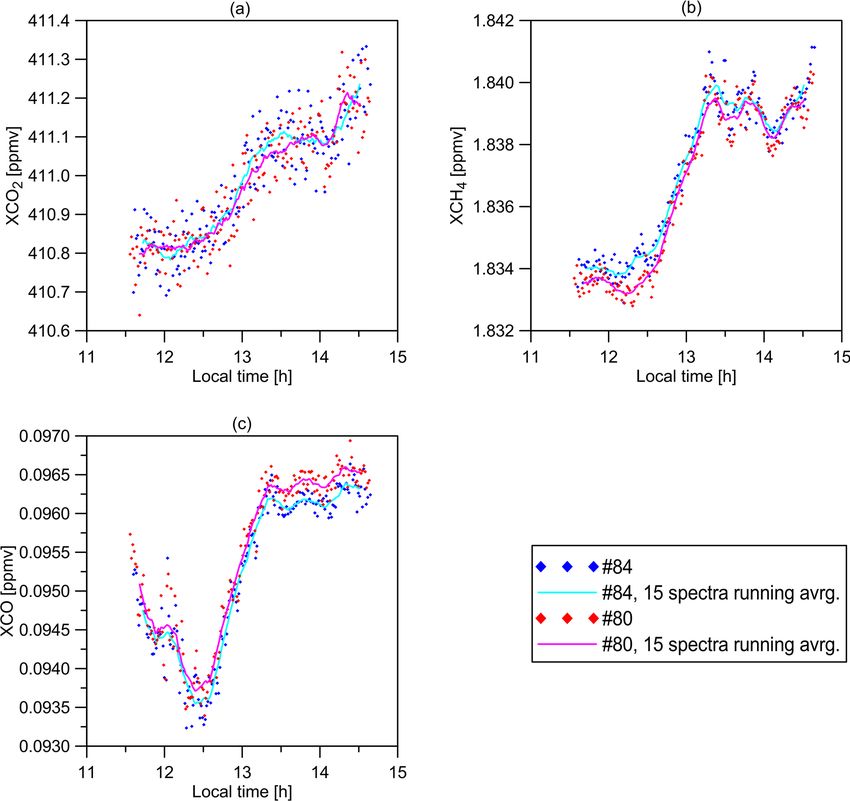
M. V. Makarova et al.: Emission Monitoring Mobile Experiment (EMME)                                                              1055

Figure 5. The scaled results of the side-by-side measurements of XCO2 , XCH4 and XCO by FTS no. 80 and FTS no. 84 on 12 April 2019.

  – in situ measurements of a Vaisala WXT520 weather                     Grid models are the best-suited tools to handle
    transmitter with an ultrasonic wind sensor, installed                the regional features of these chemicals. However,
    locally on the roof of the building of the Institute                 these models are not designed to resolve pollutant
    of Physics of SPbU (∼ 60 m a.s.l.; 59.88◦ N, 29.83◦ E;               concentrations on local scales. Moreover, for many
    point A1 in Fig. 2), hereafter referred to as “LOCAL”;               species of interest, having reaction timescales that
                                                                         are longer than the travel time across an urban area,
  – the data of Global Data Assimilation System (GDAS)                   chemical reactions can be ignored in describing lo-
    from the NCEP GFS model, which is similar to the one                 cal dispersion from strong individual sources mak-
    used to initialise the HYSPLIT dispersion calculations               ing Lagrangian and plume-dispersion models prac-
    as specified in Sect. 3, hereafter referred to as “GDAS”;            tical.
  – the wind speed and direction data retrieved from the
    backward trajectory calculations of HYSPLIT at the                 Stein et al. (2007) classify HYSPLIT as a local model
    location of downwind FTIR observation, hereafter re-            which provides “the more spatially resolved concentrations
    ferred to as “HYSPLIT”.                                         due to local emission sources”. Therefore, for modelling of
                                                                    the evolution of the St. Petersburg plume we used the HYS-
   We selected HYSPLIT as one of the sources of the wind            PLIT model as a tool which perfectly fits the scale of con-
data since HYSPLIT is a widely used modelling system                sidered atmospheric processes. This was also the reason for
for the simulation of air parcel trajectories and the dis-          using HYSPLIT as the source of the wind data.
persion processes in the atmosphere which was tested in                Both GDAS and HYSPLIT wind data are taken at the al-
a lot of studies (HYSPLIT publications can be found us-             titude level that approximately corresponds to the middle of
ing the following links: https://www.arl.noaa.gov/hysplit/          the daytime boundary layer height. An average wind is cal-
hysplit-publications-meteorological-data-information/, last         culated for the time period of FTIR observations. Result-
access: 2 March 2020). Stein et al. (2007) noted the follow-        ing wind speeds and directions from the three different data
ing:                                                                sources are given in Table A3 (see Appendix A). As ex-

https://doi.org/10.5194/amt-14-1047-2021                                              Atmos. Meas. Tech., 14, 1047–1073, 2021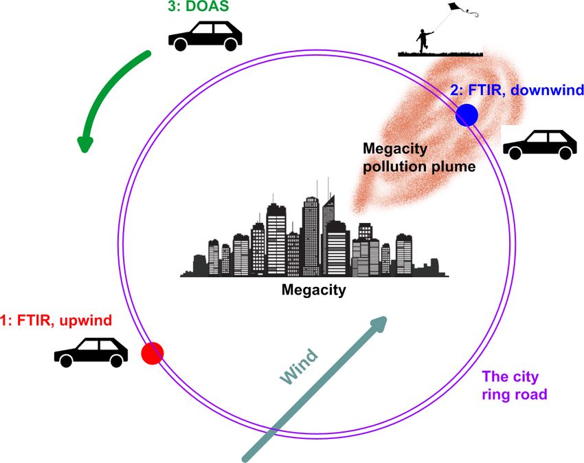
1056                                              M. V. Makarova et al.: Emission Monitoring Mobile Experiment (EMME)

pected, wind speeds at elevated altitude levels from GDAS           an east–west direction (59.60–60.29◦ N, 29.05–31.33◦ E).
and HYSPLIT are much higher than the surface wind speeds            It has been assumed that there are no significant emis-
(see Appendix A, Table A2). On some days, e.g. 6 and                sion sources outside this domain. The model resolution
18 April, in situ wind directions (LOCAL) differ consider-          (grid size) is 25 m × 25 m. The following major land use
ably from GDAS and HYSPLIT, although the latter two are             classes are considered: residential buildings/industrial ar-
consistent with each other. Note that compared to surface,          eas, roads/highways, water bodies, parks/forests/fields and
the elevated wind directions better reproduce the city plume        swamps/wetlands. In Fig. 6 these land use classes are shown
movement – e.g. northwest winds and west-northwest winds            in different colours: blue for the water bodies, grey for
on 21 and 27 March and 1 April (see Fig. 3) instead of west-        the residential buildings/industrial areas and green for the
southwest winds at the surface (see Appendix A, Table A2).          parks and forests. Effective path length is calculated as the
                                                                    sum of elementary paths through the urbanised grid pix-
4.5    Air parcel path length                                       els which contain residential buildings, industrial areas and
                                                                    roads/highways. Pixels containing water bodies, swamps and
The determination of the air parcel path length L (Eq. 2) is a      parks are excluded from the variable path calculations. A
sophisticated task due to the fact that the application of a box    similar approach was implemented by Hase et al. (2015). The
model suggests that the pollutants are well mixed in the en-        total urbanised area of the St. Petersburg agglomeration ac-
tire air box volume, but this is not true, especially for megaci-   cording to the developed land use classification occupies the
ties with a complex structure of urban terrain and distribution     area of 984 km2 , while the entire area of St. Petersburg is offi-
of emission sources. Thus, different approaches have been           cially reported to be 1439 km2 . The target gases can originate
tested to calculate L:                                              from different emission source categories; i.e. CH4 could
                                                                    partly come from the waterways (sewers and water canals),
  – A simplified box model setup with a constant path
                                                                    wetlands and pipelines rather than mobile and point combus-
    length Lj (ti ) = L = const was employed for each day
                                                                    tion sources which are relevant for CO, CO2 and NO2 . The
    of field observations. The box is designed to represent
                                                                    EMME-2019 was carried out during March–April when the
    the major part of the high-density residential and in-
                                                                    water bodies and earth surface were fully or partly covered
    dustrial area of the St. Petersburg agglomeration, so
                                                                    by ice and snow (see Appendix A, Fig. A1), and soils were
    that the respective L value is derived from the value
                                                                    still frozen. Therefore we suggest that CH4 emission from the
    of that area. Since the locations of our field observa-
                                                                    excluded pixels (water bodies, swamps, parks, and forests)
    tions are mostly placed on the outer side of the ring
                                                                    was negligible in comparison to other anthropogenic sources
    road, this road was set to be a boundary for the target
                                                                    (landfills, pipelines and sewage treatment plants, etc.) which
    emission area. Accordingly, given that the land area in-
                                                                    are distributed over the urbanised pixels.
    side the√ring is equal to 706 km2 , we get an estimate
                                                                       To minimise errors that may occur due to the land use mis-
    of L = 706 ≈ 27 km. Hereafter the results of data in-
                                                                    classification, and to take into account the airflow spatial ex-
    terpretation by means of this approach are indicated
                                                                    tension, the 10 km wide band of 11 equidistant and parallel
    by “Lconst ”.
                                                                    paths is analysed, and an average path length is calculated.
  – The variable effective path is calculated using the actual      Finally, the difference between the “polluted” path (back-
    wind direction and the land use pattern on the route of         ward from the downwind location) and “clean” path (back-
    the linear air trajectory. Only those sections of path are      ward from the upwind location) provides an estimate of the
    being taken into account that cross the area of supposed        effective path L. Figure 6 presents an example of linear back-
    anthropogenic emission. The input wind directions are           ward paths for the days of FTIR observations with the major
    those mentioned in Table A3 (see Appendix A), and the           land use classes shown by different colours.
    resulting path length calculations hereafter are indicated
    as “LLOCAL “, “LGDAS ” and “LHYSPLIT ”. The use of the          4.6   Case study: two examples
    effective path in Eq. (2) takes into account the inhomo-
    geneity of the anthropogenic emissions in the megacity          In order to illustrate the interpretation of experimental data
    to some extent.                                                 and describe the main error sources of final results, we con-
                                                                    sider 2 d of field measurements. The first one, 4 April, seems
   For the purpose of effective paths calculation, a special        to be the most successful in terms of observational condi-
gridded model of land use coverage has been constructed             tions, functioning of the equipment, data quality and clar-
on the basis of the visual classification of a publicly avail-      ity of the interpretation. It is characterised by stable weather
able map (https://yandex.ru/maps/2/saint-petersburg/?ll=30.         conditions with a moderate south-southwest wind, similarly
163886%2C59.911377&z=11, last access: 28 January 2020)              identified by different wind data sources – from the surface
that covers the St. Petersburg agglomeration with its sur-          (see Appendix A, Table A2) to higher altitude levels (see
roundings (see Fig. 6). The spatial domain of the model             Appendix A, Table A3). The simulated city plume picture
covers 76 km in a south–north direction and 128 km in               demonstrates a jet-like flow of air mass on that day, with an

Atmos. Meas. Tech., 14, 1047–1073, 2021                                               https://doi.org/10.5194/amt-14-1047-2021
M. V. Makarova et al.: Emission Monitoring Mobile Experiment (EMME) 1057 Figure 6. An example of linear backward paths (black straight lines; black dots show the downwind FTS locations) for the days of FTIR observations. The major land use classes are shown by different colours (blue for the water bodies, grey for the residential buildings/industrial areas and green for the parks and forests). The path lengths on the map are plotted as equal only for illustrative purposes. In fact they are all different since the FTIR observation locations and the wind field change from day to day. The red line designates the official administrative boundary of the St. Petersburg agglomeration. The red star indicates the location of a the major thermal power station (TPS) located to the north of St. Petersburg. Map data © 2019 Yandex. almost perfect location of both FTSs, upwind and downwind late matter (PM10 ) was very high and exceeded 60 µg m−3 almost on one line (see Fig. 3). In addition, according to the (http://www.infoeco.ru/, last access: 4 March 2020). A high- model simulation for 4 April, the upwind FTS was located pollution event was also recorded by the CIMEL sun pho- in the clean area, while the downwind one was installed very tometer installed at St. Petersburg State University (point A1, close to the plume jet. Another example is 25 April, when Fig. 2) within the AERONET international programme both FTS locations appeared to be inside the polluted area. (Volkova et al., 2018): the daily averaged value of aerosol This happened due to the specific weather conditions that optical thickness (AOT) at 500 nm was found to be 0.40 on contribute to the accumulation of air pollutants in the bound- 25 April, which is considerably higher than its long-term av- ary layer: a calm night before and light winds of 1 m s−1 in erage value (0.12 for the period of 2013–2019); a similar in- the daytime (see Appendix A, Tables A2 and A3). More- crease of AOT was recorded by the satellite measurements of over, the wind direction on 25 April at the surface (south- the MODIS satellite instrument over St. Petersburg on that southwest, Table A2) is very different from that in the middle day. of the boundary layer (east and east-northeast; Table A3). The TC data of CO2 measurements on 4 and 25 April, with According to the analysis of the air samples collected in 15 min running averages, are presented in Fig. 7. Compared air bags, the surface air on 25 April was extremely pol- to 4 April, the TC of CO2 on 25 April demonstrates higher luted. The downwind NO2 concentration was found to be levels and variation, both at upwind and downwind locations. 138 µg m−3 , while it was varying within the range of 12– Although the upwind TC is generally below the downwind 74 µg m−3 during the other days of field observations. An- level, as expected, the upwind TC starts to exceed the down- other indication of heavy anthropogenic pollution comes wind level at the end of FTS observations on 25 April. Ac- from the data of our mobile DOAS measurements: the max- cordingly, while the “downwind–upwind” difference is rel- imum of NO2 TrC recorded along the circular route was atively stable within the range of 2–4 × 10¹⁹ molec. cm−2 92 × 1015 molec. cm−2 on 25 April, while it was in the range on 4 April, it reaches 10 × 1019 molec. cm−2 at 12:00 of 15–58 × 1015 molec. cm−2 on the other days of field ob- on 25 April but becomes zero and then negative (up to servations. According to the data of municipal air quality −1 × 10¹⁹ molec. cm−2 ) after 14:30. In order to explain this monitoring, the daily average concentration of the particu- behaviour, a special run of the HYSPLIT dispersion model https://doi.org/10.5194/amt-14-1047-2021 Atmos. Meas. Tech., 14, 1047–1073, 2021
1058                                            M. V. Makarova et al.: Emission Monitoring Mobile Experiment (EMME)

was performed, with an output of CO2 TC within a bound-          and 4 April. The first requirement was the wind field sta-
ary layer every 15 min, at both FTS locations, upwind and        bility. The analysis of the wind field stability during each
downwind (see Fig. 7). As the first approximation, the CO2       day was carried out using the GDAS and HYSPLIT mete-
emission sources were assumed to be located similarly to         orological data, as well as local meteorological observations.
the NOx emission sources but scaled to match the level of        The second criterion was the homogeneity of the megacity
our FTS measurements. These calculations qualitatively re-       pollution plume. It was estimated on the basis of the anal-
produce the time series of the CO2 measurements and the          ysis of the daily variability of enhancement ratios EnhR =
different character of the results of field experiments on 4     1TC,gas1 /1TC,gas2 . The EnhR values for the following pairs
and 25 April. Moreover, we can suggest that the origin of        were considered: CO/CO2 and CH4 /CO2 . For selected days,
high CO2 TC values observed at the upwind FTS location on        the upper limit of the daily relative variability of EnhR was
25 April was the thermal power station located about 5 km        set to 30 %.
towards north from the upwind point (see Fig. 6). When the          As has been described above, there were several different
emission by the thermal power station is turned off in the       scenarios of the F calculations in which different sources of
HYSPLIT calculation, the CO2 TC drops down to the level          meteorological information (LOCAL, GDAS and HYSPLIT)
of upwind FTS measurements on 4 April (see Fig. 7b, dashed       and different methods of the air parcel path calculations were
blue line).                                                      used. The comparison of the obtained results has shown that
   The time series of Xgas for CO2 , CO and CH4 obtained         the minimum variability of F is observed when the HYS-
from the data of FTS measurements on 4 and 25 April are          PLIT meteorological data are combined with the variable ef-
shown in Fig. 8. Since the Xgas variability at clean location    fective path L (see Sect. 4.5). When selecting the results for
(upwind) is usually much smaller as compared to a polluted       final analysis, we suggest that the application of the criterion
location, it is possible to use time extrapolation of measured   of minimal variability is a good choice because in this case
data for the periods with data gaps. Figure 9 demonstrates       the corresponding estimates of area flux are more reliable.
the difference between TC for each of three gases measured       This statement can be confirmed in particular by comparison
by upwind and downwind FTS on 4 and 25 April; the ex-            of the CO2 fluxes obtained for the 9 and 4 d sets (Table 1,
trapolated data are specially marked. Figure 9 also shows the    columns 2 and 3). For the 4 d set, the variability is consid-
wind speed and wind direction for the time period of FTS         erably lower (12 kt km−2 yr−1 vs. 28 kt km−2 yr−1 ), and we
observations by the LOCAL weather station (see Sect. 4.3).       should reiterate that these 4 d were the days with the most
                                                                 favourable observational conditions during the observational
                                                                 campaign. So, we do not present the results of all scenarios
5     Results and discussion                                     and show in Table 1 (columns 2 and 3) the values obtained
                                                                 for the combination of HYSPLIT meteorological data with
5.1    Overview of obtained results                              the variable effective path. As supplementary information, in
                                                                 Appendix B we provide Table B1, which contains the values
The campaign consisted of 11 d of field measurements. On         of area fluxes for CO2 , CH4 , CO and NOx obtained using the
30 April clouds (altocumulus translucidus) started to de-        constant path length approach.
velop quickly during the field experiment (see Appendix A,          If we compare the flux values obtained for the 4 and 9 d
Table A1 and Fig. A1). On 18 April the upwind FTS lo-            sets, we see that the fluxes for CO2 are the same, but the
cation was close to the thermal power station. Owing to          fluxes for CH4 and CO are different (Table 1, columns 2
the prevailing north-northeast wind (see Appendix A, Ta-         and 3). The fluxes estimated for the selected 4 d appeared to
ble A3), the upwind FTS location appeared to be polluted         be 1.3 times higher than corresponding values obtained for
on 18 April (see Fig. 3). Consequently, 18 and 30 April were     all 9 d of field observations. The uncertainty of the obtained
excluded from final analysis, and the evaluation of the target   flux values for the 4 d subset decreased for CO2 and CH4 . We
fluxes (F ) of the investigated gases was limited to the re-     stress that during these selected 4 d not only did the specific
maining 9 d of campaign. For these 9 d the cross-correlations    meteorological conditions correspond in the best way to the
(Pearson’s correlation coefficient r) between 1TC values ob-     assumptions of the box model, but also the locations of the
tained for the pairs CO/CO2 and CH4 /CO2 were calculated:        observational points were nearly perfect.
rCO/CO2 = (0.88 ± 0.02) and rCH4 /CO2 = (0.82 ± 0.03). The          The summary of the EMME-2019 results and the compar-
high correlation is the evidence of the fact that the measure-   ison with the flux estimates for St. Petersburg based on in situ
ments in most cases were conducted inside the plume com-         measurements, as well as independent literature data, are pre-
ing from a regional/mesoscale, relatively compact powerful       sented in Table 1 for CO2 , CH4 , CO and NOx (the latter were
source of emission. We can attribute this source to the centre   derived from mobile DOAS measurements of tropospheric
of St. Petersburg.                                               NO2 in the vicinity of upwind and downwind FTIR obser-
   To further consolidate our flux estimates, some additional    vations). Prior to analysis of the results, a short overview of
restrictions were imposed on the experimental data, which        the error and uncertainty analysis should be presented. The
resulted in keeping only 4 d out of 9: 21 and 27 March and 3     random uncertainty of mean F values of CO2 , CH4 , CO and

Atmos. Meas. Tech., 14, 1047–1073, 2021                                           https://doi.org/10.5194/amt-14-1047-2021
M. V. Makarova et al.: Emission Monitoring Mobile Experiment (EMME) 1059
Figure 7. Time series of the CO2 TC measurements by mobile FTSs at upwind (U, blue) and downwind (D, red) locations on 2 d, (a) 4 and
(b) 25 April 2019. The measurements are compared with the results of the HYSPLIT simulations at both locations, upwind and downwind.
For the day of 25 April, a special HYSPLIT scenario is added for comparison: the emission of the major thermal power station (TPS) of
St. Petersburg nearby the upwind FTS location is turned off (“no TPS”; see Fig. 8 and the text for details).
Table 1. Area fluxes for CO2 (kt km−2 yr−1 ), CH4 (t km−2 yr−1 ), CO (t km−2 yr−1 ) and NOx (t km−2 yr−1 ) obtained during EMME-2019
and the flux estimates for St. Petersburg based on in situ measurements. The values previously reported in literature are also presented.
Area flux EMME In situ Literature sources
measurements
(9 d) (4 d) St. Petersburg The world’s cities
1 2 3 4 5 6
CO2 , 89 ± 28 85 ± 12 40 ± 30 31 (Serebritsky, 2018), 29 (London; O’Shea et al., 2014)
kt km−2 yr−1 46 (EDGAR database, 2018; 35.5 (London; Helfter et al., 2011)
Crippa et al., 2019) 12.8 (Mexico City; Velasco et al., 2005)
6 (suburbs; Makarova et al., 2018) 12.3 (Tokyo; Moriwaki and Kanda, 2004)
0.8–7.7 (Krakow; Zimnoch et al., 2010)
28.3 (Berlin; Hase et al., 2015)
CH4 , 135 ± 68 178 ± 30 120 ± 80 25 (Serebritsky, 2018, 2019), 66 (London; O’Shea et al., 2014)
t km−2 yr−1 110 (Makarova et al., 2006), 7–28 (Krakow; Zimnoch et al., 2010)
44 (suburbs; Makarova et al., 2018)
32 (suburbs; Zinchenko et al., 2002)
CO, 251 ± 104 333 ± 103 90 ± 50 410 (Serebritsky, 2018, 2019), 106 (London; O’Shea et al., 2014)
t km−2 yr−1 390 (Makarova et al., 2011), 1520 (Mexico City; Stremme et al., 2013)
90 (suburbs; Makarova et al., 2018)
NOx , 66 ± 28 – – 69 (Serebritsky, 2018, 2019) 63–252 (London; Lee et al., 2015)
t km−2 yr−1 13–300 (Norfolk; Marr et al., 2013)
NOx indicated in Table 1 was calculated as the standard de- random uncertainty of F for a single day of measurements
viation (SD) of daily means of area fluxes. This uncertainty (daily uncertainty) can be estimated using the following ex-
includes two components. The first component is the nat- pression:
ural flux variability, and the second component comprises
the random measurement errors and the errors introduced δF = δV + δL + δ1TC , (4)
by approximations and simplifications of the model approach where δV is the relative variation of the wind speed over
which was used. It should be specially emphasised that these a day estimated using HYSPLIT meteorological data, δL
two components cannot be identified separately. Therefore, is the relative uncertainty of the air parcel path length and
below we will use the terms “variability” or “uncertainty”, δ1TC is the relative daily variation of 1TC . The δF values
keeping in mind that these terms denote natural variations, calculated in this way can be considered as an upper limit of
measurement errors and model errors together. The relative the F uncertainty. The average values of δL, δV and δ1TC
https://doi.org/10.5194/amt-14-1047-2021 Atmos. Meas. Tech., 14, 1047–1073, 2021You can also read


