How oscillating aerodynamic forces explain the timbre of the hummingbird's hum and other animals in flapping flight
←
→
Page content transcription
If your browser does not render page correctly, please read the page content below
RESEARCH ARTICLE

                                     How oscillating aerodynamic forces
                                     explain the timbre of the hummingbird’s
                                     hum and other animals in flapping flight
                                     Ben J Hightower1†, Patrick WA Wijnings2†, Rick Scholte3, Rivers Ingersoll1,
                                     Diana D Chin1, Jade Nguyen1, Daniel Shorr1, David Lentink1*
                                     1
                                       Mechanical Engineering, Stanford University, Stanford, United States; 2Electrical
                                     Engineering, Eindhoven University of Technology, Eindhoven, Netherlands;
                                     3
                                       Engineering, Sorama, Eindhoven, Netherlands

                                     Abstract How hummingbirds hum is not fully understood, but its biophysical origin is encoded
                                     in the acoustic nearfield. Hence, we studied six freely hovering Anna’s hummingbirds, performing
                                     acoustic nearfield holography using a 2176 microphone array in vivo, while also directly measuring
                                     the 3D aerodynamic forces using a new aerodynamic force platform. We corroborate the acoustic
                                     measurements by developing an idealized acoustic model that integrates the aerodynamic forces
                                     with wing kinematics, which shows how the timbre of the hummingbird’s hum arises from the
                                     oscillating lift and drag forces on each wing. Comparing birds and insects, we find that the
                                     characteristic humming timbre and radiated power of their flapping wings originates from the
                                     higher harmonics in the aerodynamic forces that support their bodyweight. Our model analysis
                                     across insects and birds shows that allometric deviation makes larger birds quieter and elongated
                                     flies louder, while also clarifying complex bioacoustic behavior.

*For correspondence:                 Introduction
dlentink@stanford.edu                Birds, bats, and insects flap their wings to generate unsteady aerodynamic forces that lift their body
†
 These authors contributed           into the air, which enables them to fly. When their flapping wings move through air, they create
equally to this work                 unsteady pressure fluctuations that radiate outward at the speed of sound. In addition to furnishing
                                     flight, pressure waves serve various acoustic communication functions during behavioral displays.
Competing interest: See
                                     Male Drosophila use aerodynamically functional wings to create humming songs near their flapping
page 19
                                     frequency to increase female receptivity to mating (von Schilcher, 1976). In a more sophisticated
Funding: See page 19                 form of courtship behavior, male and female mosquitoes duet at the third harmonic (multiple) of
Received: 15 September 2020          their wingbeat frequency (Cator et al., 2009). In contrast, pigeons use modified primary feathers
Accepted: 28 February 2021           that sonate around 1 kHz when they start flapping their wings that incite flock members to fleeing
Published: 16 March 2021             and take-off behavior (Davis, 1975; Hingee and Magrath, 2009; Niese and Tobalske, 2016;
                                     Murray et al., 2017). Feather sonation during flapping flight may also communicate information like
Reviewing editor: Gordon J
Berman, Emory University,
                                     flight speed, location in 3D space, and wingbeat frequency to conspecifics (Larsson, 2012). Hence,
United States                        male broad-tailed hummingbirds generate a whistling sound with modified primary feathers in their
                                     flapping wings during displays to defend courting territories (Miller and Inouye, 1983). Silent fliers
   Copyright Hightower et al.
                                     like owls, on the other hand, suppress the aerodynamic sound generated by their wings to mitigate
This article is distributed under
                                     interference with their hearing and escape prey detection (Geyer et al., 2013; Jaworski and Peake,
the terms of the Creative
Commons Attribution License,         2020; Kroeger et al., 1972; Sarradj et al., 2011; Clark et al., 2020). Their flapping wings also gen-
which permits unrestricted use       erate less structural noise (Clark et al., 2020) because their feathers lack the noisy directional fasten-
and redistribution provided that     ing mechanism that locks adjacent flight feathers during wing extension in other bird species
the original author and source are   (Matloff et al., 2020). These diverse adaptations illustrate how a wide range of mechanisms can
credited.                            contribute to the sound that flapping wings generate. Consequently, it is not fully understood how

Hightower, Wijnings, et al. eLife 2021;10:e63107. DOI: https://doi.org/10.7554/eLife.63107                                              1 of 31
Research article                                                                                            Evolutionary Biology

                                   eLife digest Anyone walking outdoors has heard the whooshing sound of birdwings flapping
                                   overhead, the buzzing sound of bees flying by, or the whining of mosquitos seeking blood. All
                                   animals with flapping wings make these sounds, but the hummingbird makes perhaps the most
                                   delightful sound of all: their namesake hum. Yet, how hummingbirds hum is poorly understood.
                                      Bird wings generate large vortices of air to boost their lift and hover in the air that can generate
                                   tones. Further, the airflow over bird wings can be highly turbulent, meaning it can generate loud
                                   sounds, like the jets of air coming out of the engines of aircraft. Given all the sound-generating
                                   mechanisms at hand, it is difficult to determine why some wings buzz whereas others whoosh or
                                   hum.
                                      Hightower, Wijnings et al. wanted to understand the physical mechanism that causes animal
                                   wings to whine, buzz, hum or whoosh in flight. They hypothesized that the aerodynamic forces
                                   generated by animal wings are the main source of their characteristic wing sounds. Hummingbird
                                   wings have the most features in common with different animals’ wings, while also featuring
                                   acoustically complex feathers. This makes them ideal models for deciphering how birds, bats and
                                   even insects make wing sounds.
                                      To learn more about wing sounds, Hightower, Wijnings et al. studied how a species of
                                   hummingbird called Anna’s hummingbird hums while drinking nectar from a flower. A three-
                                   dimensional ‘acoustic hologram’ was generated using 2,176 microphones to measure the humming
                                   sound from all directions. In a follow-up experiment, the aerodynamic forces the hummingbird wings
                                   generate to hover were also measured. Their wingbeat was filmed simultaneously in slow-motion in
                                   both experiments. Hightower, Wijnings et al. then used a mathematical model that governs the
                                   wing’s aeroacoustics to confirm that the aerodynamic forces generated by the hummingbirds’ wings
                                   cause the humming sound heard when they hover in front of a flower. The model shows that the
                                   oscillating aerodynamic forces generate harmonics, which give the wings’ hum the acoustic quality
                                   of a musical instrument.
                                      Using this model Hightower, Wijnings et al. found that the differences in the aerodynamic forces
                                   generated by bird and insect wings cause the characteristic timbres of their whines, buzzes, hums, or
                                   whooshes. They also determined how these sounds scale with body mass and flapping frequency
                                   across 170 insect species and 80 bird species. This showed that mosquitos are unusually loud for
                                   their body size due to the unusual unsteadiness of the aerodynamic forces they generate in flight.
                                      These results explain why flying animals’ wings sound the way they do – for example, why larger
                                   birds are quieter and mosquitos louder. Better understanding of how the complex forces generated
                                   by animal wings create sound can advance the study of how animals change their wingbeat to
                                   communicate. Further, the model that explains how complex aerodynamic forces cause sound can
                                   help make the sounds of aerial robots, drones, and fans not only more silent, but perhaps more
                                   pleasing, like the hum of a hummingbird.

                                   flapping wings generate their characteristic sound—from the mosquito’s buzz, the hummingbird’s
                                   hum, to the larger bird’s whoosh.
                                       Our physical understanding of how wings generate sound is primarily based on aircraft wing and
                                   rotor aeroacoustics (Brooks and Pope, 1989; Crighton, 1991). In contrast to animals, however,
                                   engineered wings do not flap, do not change shape dynamically, are much larger, and operate at
                                   much higher speeds (higher Reynolds numbers). They also operate at lower angles of attack to avoid
                                   stall, which results in more compact airflow patterns than animals generate in flapping flight
                                   (Ellington et al., 1996; Dickinson et al., 1999; Mueller, 2001). Despite these marked differences,
                                   rotors and flapping wings have one thing in common: they both revolve around a center pivot.
                                   Whereas flapping wings reciprocate along the joint, rotors revolve unidirectionally. The revolution of
                                   rotors generates loud tonal noise, because the pressure field they generate rotates in space at the
                                   same frequency (Lighthill, 1954; Lowson, 1965). Similarly, when animals flap their wing back and
                                   forth along the shoulder joint during each stroke, they create a high-pressure region below their
                                   wing and a low-pressure region above. The pressure differences are associated with the wing’s high
                                   lift and drag, respectively (Sane and Dickinson, 2001; Wu and Sun, 2004). Computational fluid

Hightower, Wijnings, et al. eLife 2021;10:e63107. DOI: https://doi.org/10.7554/eLife.63107                                          2 of 31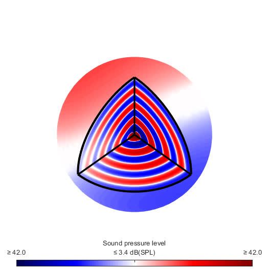
Research article Evolutionary Biology
A D G
fs Fwing L
hs aa
R3
fp
α x
D vR3 y z
θ
-Φ
wing movement
fs
p
^ ^
r^ × D
B D
E 10 -3 H
(-)stroke and deviation [°]
^
3 D r^ r^ ^
r^ × D 5 90
vR3 vR3 60
pressure [Pa]
lift and drag
2
normalized
30
1 0 0
-30
0
-60
-1 -5 -90
0 50 100 0 50 100 0 50 100
wingbeat % wingbeat % wingbeat %
C 1 F I 1
stroke and deviation
60
normalized power
normalized power
sound pressure
0.5 0.5
lift and drag
level [dB]
0 40 0
1 1
20
0.5 0.5
0 0 0
1 2 3 4 1 2 3 4 5 6 7 8 9 10 1 2 3 4
harmonic harmonic harmonic
Figure 1. Oscillating aerodynamic force and acoustic field measurements to determine how hummingbirds hum. (A) 3D aerodynamic force platform
setup to measure the forces generated by a hovering hummingbird. Each of the flight arena’s walls comprises a force plate (fp) instrumented by three
force sensors (fs), two additional force sensors instrument the perch. The six DLT calibrated cameras imaging through three orthogonal ports in pairs
are not shown. (B) The lift and drag force generated by hovering hummingbirds during a wingbeat (gray area, downstroke; mean ± std based on N = 6
birds, each bird made two flights, n = 5 wingbeats were fully analyzed per flight for 60 total wingbeats). Lift is negative during the upstroke since the
direction of the lift vector is perpendicular to the wing velocity while the drag vector is parallel and opposite to the wing velocity direction, resulting in
the lift vector being defined as the cross product of the wing velocity direction and the drag direction (inset). (C) Most of the frequency content in the
lift profile is contained in the first harmonic and corresponds to the high forces generated during downstroke (first harmonic mean ± standard deviation
is 44.2 ± 1.8 Hz across all birds and flights). In contrast, the frequency content in the drag profile is contained primarily in the second harmonic and
corresponds to the equivalent drag generated during the up and downstroke. (D) Acoustic flight arena in which hovering hummingbirds (N = 6 birds,
n = 2 flights per bird) were surrounded by four acoustic arrays (labeled aa; 2 1024 and 2 64 microphones) and four high-speed cameras (hs) while
feeding from a stationary horizontal flower (separate experiment with six other individuals). (E) Throughout a wingbeat, each microphone records the
local acoustic field generated by the hovering hummingbird (microphone located at the center above bird #1). (F) To generate a representative
spectrum of a single bird, the signals of all microphones in all arrays around the bird were summed (green line: N = 1, n = 1) and plotted up to the
tenth harmonic. The background spectrum of the lab (range over all trials) is plotted in gray, showing the hum consists primarily of tonal noise higher
than the background at wingbeat harmonics (dark green line, 3 dB above maximum background noise). In addition, several smaller non-harmonic tonal
peaks can be observed between the first and fourth harmonic with a dB level equivalent to the sixth - seventh harmonic. (G) To determine the acoustic
source of the hum, we constructed a simple model that predicts the acoustic field. The acoustic waves radiate outwards from the overall oscillating
force (Fwing ) generated by each wing, which can be decomposed into the lift (L) and drag (D) forces generated by each wing (recorded in vivo, B). To
predict the aeroacoustics, these forces are positioned at the third moment of inertia of the wing (R3 ) and oscillate back and forth due to the periodic
flapping wing stroke (j) and deviation angle (q) (recorded in vivo, H). Angle of attack a is defined for modeling flapping wing hum across flying species
(Figure 4). (I) Hummingbird wing kinematics (j, q) measured in vivo from the 3D aerodynamic force platform experiment (gray area, downstroke; mean
± std based on N = 6 birds, n = 2 flights). (I) Whereas most of the frequency content in the stroke profile is contained in the first harmonic, the content
in the deviation profile extends to the second and third harmonics.
dynamics (CFD) simulations of flapping insect wings suggest that the acoustic field can be character-
ized as a dipole at the wingbeat frequency (Bae and Moon, 2008; Geng et al., 2017; Seo et al.,
2019). Further, flapping wing pitch reduction (Nedunchezian et al., 2018) and increased wing
Hightower, Wijnings, et al. eLife 2021;10:e63107. DOI: https://doi.org/10.7554/eLife.63107 3 of 31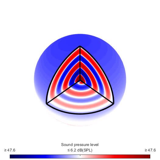
Research article                                                                                             Evolutionary Biology

                                   flexibility (Nedunchezian et al., 2019) reduces the simulated nearfield sound pressure level. All
                                   these findings point to the potential role of oscillating aerodynamic forces in generating wing hum.
                                   Indeed,       numerical      simulation      of     the     Ffowcs      Williams     and       Hawkings
                                   aeroacoustic equation (Williams and Hawkings, 1969) showed that the farfield hum of flapping
                                   mosquito wings is primarily driven by aerodynamic force fluctuation (Seo et al., 2019). Despite these
                                   important advances, in vivo acoustic near-field measurements are lacking. Finally, there is no simple
                                   model that can satisfactorily integrate flapping wing kinematics and aerodynamic forces to predict
                                   the acoustic near and far field generated by animals across taxa without using computationally
                                   expensive fluid dynamic simulations.
                                       Hummingbirds are an ideal subject for developing and testing a model of flapping wing hum:
                                   their wing kinematics and unsteady aerodynamic forces are very repeatable during hover
                                   (Altshuler and Dudley, 2003; Tobalske et al., 2007; Ingersoll and Lentink, 2018). Further, hum-
                                   mingbird wing morphology and flight style share similarities with both birds and insects. In addition
                                   to high-frequency feather sonations, hummingbirds produce a prominent hum that is qualitatively
                                   similar to an insect’s buzz. Earlier aeroacoustics studies of hummingbirds have resolved the farfield
                                   acoustic pressure field at a distance greater than 10 or more body lengths away from the humming-
                                   bird (Clark and Mistick, 2018a; Clark, 2008; Clark et al., 2016; Clark and Mistick, 2018b). While
                                   this distance relates to how humans perceive and interact with these animals, hummingbirds fre-
                                   quently interact with conspecifics and other animals at more intimate distances—in the acoustic
                                   nearfield. Furthermore, wing hum can announce a hummingbird’s presence, especially to the oppo-
                                   site sex (Hunter, 2008). Although their audiogram has yet to be established below 1 kHz
                                   (Pytte et al., 2004), this and other behavioral evidence suggests hummingbirds may be able to per-
                                   ceive the wing hum from a conspecific. Finally, the hum may reveal the hummingbird’s presence to
                                   predators in plant clutter when vision is obstructed.
                                       To resolve how the oscillating aerodynamic force generated by flapping wings may contribute to
                                   wing hum, we developed a new aerodynamic force platform (Ingersoll and Lentink, 2018;
                                   Lentink et al., 2015; Hightower et al., 2017) to directly measure the net 3D aerodynamic force
                                   generated by freely hovering hummingbirds. We integrated this data in a new aeroacoustics model
                                   to predict the sound radiated due to the oscillating forces from flapping wings. Our model is ideal-
                                   ized in the sense that it assumes the wings are rigid airfoils, thereby neglecting auxiliary effects such
                                   as wingtip flutter, feather whistle and (turbulent) vortex dynamics. Next, we compared the predicted
                                   acoustic field with novel acoustic nearfield recordings for six freely hovering hummingbirds, which
                                   corroborates the predictive power of our minimal model. We then used our validated model to
                                   determine how flapping wing hum depends on the frequency content in the oscillating forces across
                                   mosquitos, flies, hawkmoths, hummingbirds, and parrotlets in slow hovering flight. Finally, we used
                                   these findings to determine how the hum scales with body mass and flapping frequency across 170
                                   insect and bird species.

                                   Results
                                   In vivo 3D aerodynamic force and acoustic nearfield measurements
                                   To determine how the flapping wings of hovering hummingbirds generate unsteady aerodynamic
                                   forces as well as their namesake acoustic humming signature, we combine aerodynamic force plat-
                                   form (Figure 1A) and microphone array recordings (Figure 1D) in vivo. The aerodynamic force plat-
                                   form integrates both the steady and unsteady components of the pressure field around the bird up
                                   to three times the wingbeat frequency, which are associated with its net 3D aerodynamic forces. In
                                   contrast, the microphone arrays measure the unsteady component of the pressure field around the
                                   bird up to ~1000 times the wingbeat frequency (of which we studied the first ten harmonics): the
                                   acoustic field. Critically, these two representations of the pressure fluctuations generated by the bird
                                   should relate mechanistically if the acoustic field of the hummingbird’s hum originates primarily from
                                   the oscillating aerodynamic lift and drag forces generated by the flapping wings.
                                       The oscillating 3D aerodynamic forces were recorded simultaneously with the wingbeat kinemat-
                                   ics using three calibrated stereo high-speed camera pairs (Figure 1A; N = 6 birds, n = 2 flights per
                                   bird, n = 5 wingbeats per flight: 60 total wingbeats). We combined the 3D aerodynamic forces, 3D
                                   wing kinematics and wing morphology measurements to decompose the oscillating lift and drag

Hightower, Wijnings, et al. eLife 2021;10:e63107. DOI: https://doi.org/10.7554/eLife.63107                                           4 of 31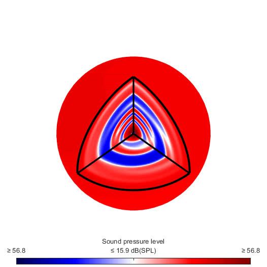
Research article                                                                                                                              Evolutionary Biology

                                            A                            70

                                             sound pressure level [dB]
                                                                         50

                                                                         30

                                                                         10

                                                                              0      100        200        300     400                  500
                                                                                                frequency [Hz]

                                                                                                                                      0
                                            B                                     measurement              model

                                                                                                                                      10
                                                                                                                                      20
                                                                                                                                      30
                                                                                                                                      40
                                                                                                                         downstroke

                                                                                                                                            wingbeat %
                                                                                                                                      50
                                                                                                                         upstroke

                                                                                                                                      60
                                                                                                                                      70

                                           pressure
                                              [Pa]

                                                                         2.0
                                                                                                                                      80

                                                                         1.5
                                                                         1.0
                                                                         0.5
                                                                         0
                                                                                                                                      90

                                                                         -0.5
                                                                         -1.0
                                                                         -1.5
                                                                                                                                      100

                                                                         -2.0

                                   Figure 2. The measured spectra and holograms match those predicted by the simple aeroacoustics model. (A) A
                                   representative acoustic spectrum measured from all arrays for hummingbird #1 in hover is shown in dark green
                                   (n = 1), while the range for N = 6 hummingbirds is shown in light green. The variation in the frequency and sound
                                   pressure level (SPL) peak value associated with each harmonic is shown with orange circles (mean) and ellipsoids
                                   Figure 2 continued on next page

Hightower, Wijnings, et al. eLife 2021;10:e63107. DOI: https://doi.org/10.7554/eLife.63107                                                                            5 of 31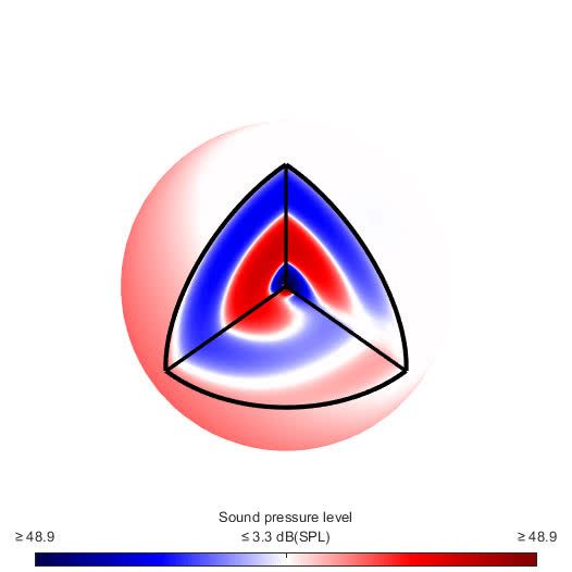
Research article                                                                                                      Evolutionary Biology

                                   Figure 2 continued
                                   (width and height, 68% confidence intervals; their asymmetric shape stems from computing the covariance in
                                   Pascals while the spectrum is in dB). The peak sound pressure levels predicted by our acoustic model (purple line)
                                   match those of the measured spectrum up to higher harmonics. In addition, several smaller non-harmonic tonal
                                   peaks can be observed between the first and fourth harmonic with a dB level equivalent to the sixth - seventh
                                   harmonic. The predicted spectrum starts at the numerical noise floor, of which the amplitude (< 10 dB) is
                                   physically irrelevant. (B) Acoustic holograms throughout the example wingbeat for hummingbird #1 (Figure 1E,F)
                                   are presented side-by-side as measured (left) and modeled (right) for the top and front array microphone
                                   positions. There is reasonable spatial and temporal agreement between the measured and predicted acoustic
                                   nearfield centered around stroke transition (30–70%) where the pressure transitions from minimal (blue) to maximal
                                   (red).
                                   The online version of this article includes the following figure supplement(s) for figure 2:
                                   Figure supplement 1. Spectra and holograms show agreement between a 10-element distributed source model
                                   and the equivalent single point source model.
                                   Figure supplement 2. Spectra shows good agreement between full model and simplified model.
                                   Figure supplement 3. Illustration of regularization for lift and drag.
                                   Figure supplement 4. Choice of regularization constants does not appreciably affect smoothing.
                                   Figure supplement 5. Spectra of all inputs into the acoustic model reveal the source of humming harmonics and
                                   evidence of frequency mixing.
                                   Figure supplement 6. Agreement between calculated lift and weight support in the vertical direction.
                                   Figure supplement 7. Sensitivity of the spectrum to the location of the acoustic point force along the wing radius.

                                   forces that each wing generates throughout the wingbeat (Figure 1B,C). The oscillating lift trace
                                   consists primarily of the peak force generated during downstroke, which corresponds to a peak in
                                   its spectrum at the first wingbeat harmonic (44.2 ± 1.8 Hz). The drag trace consists of two equivalent
                                   drag peaks during the upstroke and downstroke, which corresponds to a dominant peak in its spec-
                                   trum at the second harmonic. We also measured the 3D beak contact force on the artificial flower
                                   from which the hummingbird was feeding, which is negligible (5.2 ± 2.3% bodyweight).
                                       The 3D acoustic field associated with the bird’s hum was quantitatively reconstructed from meas-
                                   urements recorded in a custom flight arena using four acoustic arrays (Figure 1D; N = 6 birds,
                                   n = 18 flights total, see Supplementary file 1 for details). The recording by a single microphone cen-
                                   tered above the bird shows a typical pressure trace throughout a single wingbeat (Figure 1E). The
                                   many fluctuations explain the rich frequency content revealed in the acoustic spectrum averaged
                                   over all microphones (Figure 1F). These include strong peaks at the fundamental frequencies of the
                                   wingbeat as well as its higher harmonics, which rise prominently above the background noise floor
                                   and characterize the hummingbird hum.

                                   Aeroacoustics model of the hum synthesizes in vivo forces and wing
                                   kinematics
                                   To determine if the low frequency oscillating forces generated by the birds’ flapping wings drive the
                                   characteristic humming sound spectrum, we develop a simple aeroacoustics model based on the
                                   governing acoustics equations that predict the resulting acoustic field. Our minimal model of the
                                   acoustic pressure field radiated by the flapping wings (Figure 1G) depends only on the physical
                                   properties of air, the wing stroke kinematics (Figure 1H), and the oscillating lift and drag forces that
                                   we measured in vivo (Figure 1B).
                                       Aerodynamic analysis of propellers shows how a radial force distribution can be integrated and
                                   represented by the net force at the center of pressure, a characteristic radial location where the net
                                   force acts (Weis-Fogh, 1973). Analogously, we determine that the acoustic sound radiation of an
                                   unsteady aerodynamic force distribution over the wing can also be concentrated into an equivalent
                                   point force at the effective acoustic source location along the wing, similar to propeller noise theory
                                   (Lowson, 1965). The effective radius of this point, measured with respect to the shoulder joint, is
                                   equal to the point at which the net drag force results in the same net torque on the wing (Low-
                                   son, 1965). This radius lies at the wing-length-normalized third moment of area for flapping wings,
                                   R3 =R (Weis-Fogh, 1973). For Anna’s hummingbirds R3 =R is equal to 55% wing radius (Kruyt et al.,
                                   2014). In practice, the effective radius for acoustic calculations can differ somewhat from the effec-
                                   tive radius for a point force (Lowson, 1965). Therefore, we conduct a dimensional analysis to

Hightower, Wijnings, et al. eLife 2021;10:e63107. DOI: https://doi.org/10.7554/eLife.63107                                                     6 of 31
Research article                                                                                                         Evolutionary Biology

Figure 3. Nearfield versus farfield measured radial sound pressure level generated by a hovering hummingbird. (A) The full 3D broadband (from 3 to
500 Hz; animated in Video 1) pressure field measured over a wingbeat from bird #1 (oriented as the 3D view avatar) is shown across the spherical
circumference at 1 m radius, the acoustic nearfield (outside the wing radius of the bird, 8 cm) and at 10 m radius, the acoustic farfield (wavelength of
first wingbeat harmonic is 7.8 m). These 3D acoustic field reconstructions are based on the measurements from all arrays (Figure 1D). (B) At a nearfield
Figure 3 continued on next page

Hightower, Wijnings, et al. eLife 2021;10:e63107. DOI: https://doi.org/10.7554/eLife.63107                                                        7 of 31
Research article                                                                                                                                     Evolutionary Biology

Figure 3 continued
distance of 1 m, the 3D broadband pressure surfaces can be represented with cross sections along the two key anatomical planes, the side/sagittal and
front/coronal plane respectively, to visualize the broadband pressure directivity over the entire wingbeat. The mean pressure directivity trace for all
birds is colored dark with color coding referring to the anatomical plane, the quantiles for each of the six birds are shaded light, and model prediction
are shown in black. The overall pressure shape in 3D is plotted in the middle in black, which has a roughly spherical shape in the broadband
holograms. (C) The 3D broadband pressure directivity at a farfield distance of 10 m. The waists of the individual lobes in each flight are smeared out
due to small variations between the birds and their flights, obscuring the directivity in the average plots (individual traces shown in Figure 3—figure
supplement 1). To show where the principle axes of the individual pressure lobes fall, we calculated the waistline pressure level between the minimum
lobes and plot the directivity axis as the line perpendicular to the waistline (gray line, light gray arc ±1 SD; D, E). The broadband hologram can be
further decomposed into contributions from the first harmonic. The measurement and simulations match better for the nearfield (computationally
backpropagated) than for the farfield (computationally propagated). In the sagittal plane, the dipoles for both the measurement and model are tilted
aft. This tilt can also be observed as a rotational mode associated with the wingbeat frequency in the longitudinal direction in the 3D animation for the
first harmonic for bird #1 (Video 2). In contrast, the associated coronal dipoles are oriented vertical. The 3D pressure shape is also more oblong, as
viewed by the ovoid black shape in the middle. (F, G) The sagittal and coronal dipoles of the second harmonic are oriented vertically in both the
nearfield and farfield. This vertical orientation is associated with the vertical force generation occurring twice per wingbeat and is also visible in the 3D
animation for the second harmonic (Video 3). (H, I) We observed a rotational mode in the 3D animation for the third harmonic (Video 4). (J, K) Both the
sagittal and coronal dipoles of the fourth harmonic are oriented vertical in both the nearfield and farfield, which is also visible in the animation
(Video 5). The third and fourth harmonic are decompositions of the first two modes; therefore, they share directivity similarities. Finally, the data driven
model prediction in B-K (black contours) match the in vivo data reasonably well in amplitude considering the differences in peak spectrum amplitude
noted in Table 1. There is also good agreement in the directivity of the predicted angles for the first two harmonics for both sagittal and coronal
planes and for the first four harmonics for the coronal plane (Table 2), which matches the agreement in amplitude.
The online version of this article includes the following figure supplement(s) for figure 3:
Figure supplement 1. Individual directivity traces show waistlines.

                                      determine how acoustic pressure scales with radial position (see Supplementary Information for
                                      details), which confirms R3 is the appropriate radius. This acoustic radius agrees with wind turbine
                                      acoustics measurements at lower harmonics of the blade passing frequency (Oerlemans et al.,
                                      2001).
                                         Starting at the time and location where the acoustic wave was generated by the unsteady force
                                      on the left and right wing, we numerically solve how the acoustic wave propagates outward into
                                      space to the location where we observe it with a microphone. Mathematically, the acoustic equation
                                      describes how the unsteady aerodynamic point force, Fwing , generated by the flapping wing gener-
                                      ates an air pressure fluctuation, p, in the stationary atmosphere at the so-called ‘retarded time’, t,
                                      which radiates outward as a wave at the speed of sound, ao , as follows Lowson, 1965:
                                                                    "                                                                                                       #
                                                                                     1                     1 ð1 M 2 Þ
                                                             p¼                                                                  r  Fwing                Fwing  M
                                                                       4pjrj2 ð1 Mr Þ2 jrj ð1 Mr Þ
                                                             |fflfflfflfflfflfflfflfflfflfflfflfflfflfflfflfflfflfflfflfflfflfflfflfflfflfflfflfflfflfflfflfflfflfflfflfflfflfflfflfflfflfflfflfflfflfflfflfflfflfflfflfflfflfflfflfflffl{zfflfflfflfflfflfflfflfflfflfflfflfflfflfflfflfflfflfflfflfflfflfflfflfflfflfflfflfflfflfflfflfflfflfflfflfflfflfflfflfflfflfflfflfflfflfflfflfflfflfflfflfflfflfflfflfflffl}
                                                                                                                  nearfield
                                                                   "                                                                                                             # :  (1)
                                                                                      1                                qFwing                  1 qMr
                                                              þ                                                  r                  þ                            r  Fwing
                                                                     4pao jrj2 ð1 Mr Þ2                                   qt              1 Mr qt
                                                                   |fflfflfflfflfflfflfflfflfflfflfflfflfflfflfflfflfflfflfflfflfflfflfflfflfflfflfflfflfflfflfflfflfflfflfflfflfflfflfflfflfflfflfflfflfflfflfflfflfflfflfflfflfflfflfflfflffl{zfflfflfflfflfflfflfflfflfflfflfflfflfflfflfflfflfflfflfflfflfflfflfflfflfflfflfflfflfflfflfflfflfflfflfflfflfflfflfflfflfflfflfflfflfflfflfflfflfflfflfflfflfflfflfflfflffl}
                                                                                                                 farfield

                                         The brackets indicate that the propagating pressure values, p, are evaluated at the retarded
                                      time, t. The vectorial distance from the moving point source on the flapping wing to the stationary
                                      microphone is measured by the vector, r, in a Cartesian reference frame fixed to earth. The wing’s
                                      velocity at the radial position where the point force acts, vR3 , is nondimensionalized with the acoustic
                                                                                                                                                       def
                                      wave velocity, ao , the speed of sound, which defines in the Mach vector M ¼ vR3 =ao . The Mach num-
                                                                                                                    def
                                      ber is simply the magnitude of the Mach vector M ¼ jMj. Similarly, the convective Mach number,
                                         def
                                      Mr ¼ M  r=jrj, is simply the component of the Mach vector, M, along the vector, r, that runs from the
                                      wing source to the microphone. The acoustic pressure fluctuation, p, consists out of two compo-
                                      nents of which the respective strengths depend on how far the microphone is located away from the
                                      wing—measured in wavelengths of the acoustic frequency of interest (Howe, 2014). For a flapping
                                      hummingbird wing we choose the wingbeat frequency, because it is associated with the first har-
                                      monic we observe in the humming spectrum (Figure 1F), l1 ¼ a0 =f1 » 343=44:2 ¼ 7:8 m. The first term

Hightower, Wijnings, et al. eLife 2021;10:e63107. DOI: https://doi.org/10.7554/eLife.63107                                                                                         8 of 31
Research article Evolutionary Biology
1 10 -5 65
A 3
2
B C D
1
0 0 60
normalized power from vertical force
10 -7
3 1
sound pressure level [dB]
radiated acoustic power [W]
2
normalized vertical force
1 55
0 10 -9
0
3 1 50
2
1 10 -11
0 45
0
3 1 -13
2 10
1 40
0
0 10 -7
3 1 10 -15 35
2
1
0
0 10 -17 30
0 50 100 0 1 2 3 4 0 1 2 3 4
wingbeat % harmonic harmonic
10 0
E slope = 1.3 slope = 2.6 F slope = 0.9 slope = 1.1
R 2 = 89.3% slope = 2.0 R 2 = 95.0% slope = 1.0
slope = 2.0 slope = 2.0 slope = 1.0 slope = 1.0
radiated acoustic power [W]
2 2
R = 68.4% slope = 0.6 R = 90.5% slope = 1.0
10 -5 slope = 1.3 slope = 0.9
10 -10
10 -15
10 -6 10 -4 10 -2 10 0 10 -12 10 -10 10 -8 10 -6 10 -4
2 2 2 2
mass [kg] 4m g f /
o w
a3
o o
[W]
Figure 4. Distinct aerodynamic weight support profiles and non-allometric flapping wing scaling differentiates the acoustic spectrum and radiated
power of flapping wing hum. (A) Representative aerodynamic weight support profiles of paradigm animals representing elongated flies, compact flies,
butterflies and moths, hummingbirds, and generalist birds. The representative weight support profile was used to simulate the hum across animals in
each group, with body mass varying over seven orders of magnitude and flapping frequency over three orders of magnitude. (B) The frequency content
of these weight support profiles is distinct. Elongated flies and compact flies concentrate energy at the second harmonic and have substantial
frequency content at higher harmonics compared to hummingbirds and hawkmoths, which have high first and second harmonics. In contrast, parrotlets
concentrate most of their energy at the first harmonic. (C) Using our aeroacoustics model, we prescribed each of the five animals (gray avatars) all five
weight support profiles (red, orange, blue, green, and purple datapoints match avatars in A) to determine how this affected the total radiated acoustic
power of the wing hum (e.g. a fly was prescribed the respective weight support profiles of a mosquito, fly, hawkmoth, hummingbird, and parrotlet). The
weight support profiles of the mosquito and fly consistently generate more radiated power than the profiles of the other animals. Differences between
the paradigm animal groups across the different scales are primarily governed by nonlinear interactions between the acoustic parameters. The inset
zooms in on the model results at hummingbird scale, which reveals the marked influence of weight support profile on radiated power over one order of
magnitude. (D) At the hummingbird scale, the weight support profiles (A and B) differentiate between the overall decibel level and distribution across
the first four harmonics (to enhance readability we slightly shifted each spectrum from the harmonic to the left). (E) We find these effects across the
seven orders of magnitude across which body mass ranges for the 170 flying animals that perform flapping flight. The model is based on body mass,
wing length, and flapping frequency of each individual species combined with the weight support profile of the associated paradigm animal (A). The
computational results across all species (black line, best-fit scaling across all groups) show the simplified scaling law derived from the acoustic
equations used in the model (gray line, predicted scaling result) closely matches the computational outcome for moths and butterflies (blue line). Other
groups deviate appreciably from the acoustic scaling law prediction (colored lines, best-fit scaling per group), because their wing length and flapping
frequency scale allometrically with body mass. (F) To test if the acoustic scaling law is reasonably accurate for all groups when allometric scaling is
incorporated, we plot the simulated radiated acoustic power versus the scaling law: the product of force, stroke amplitude and flapping frequency
squared (divided by the constant product of air density and speed of sound). On average this shows good agreement between the computational
model (black line) and scaling law prediction (gray line) across all groups.
The online version of this article includes the following figure supplement(s) for figure 4:
Figure 4 continued on next page
Hightower, Wijnings, et al. eLife 2021;10:e63107. DOI: https://doi.org/10.7554/eLife.63107 9 of 31
Research article                                                                                               Evolutionary Biology

Figure 4 continued
Figure supplement 1. The multiplicative factor Rfw =ao <
                                                       ~ 0:01 is much smaller than one for all 170 animals.
Figure supplement 2. The flapping Mach number Mf <    ~ 0:1 is small for all 170 animals.

                                     in Equation 1 dominates in the nearfield close to the wing up to a wavelength away from it. The
                                     associated pressure wave has a 3D dipole shape radiating in two opposing directions. Its strength is
                                     proportional to the force vector reorientation in space with respect to the radial vector, r, pointing
                                     from the source to the microphone. The second term dominates in the farfield starting at a wave-
                                     length away from the wing. The associated pressure wave has a 3D quadrupole shape along four pri-
                                     mary directions. Its strength is proportional to the point force unsteadiness and the radial
                                     acceleration of its position in space. In the case of a hummingbird, the nearfield term decays expo-
                                     nentially with distance. This is because the hummingbird acts as a compact acoustic source
                                     (Rienstra and Hirschberg, 2004), since the wavelength at the wingbeat frequency (first harmonic) is
                                     much larger than the radius of the wing, R, the representative acoustic source length scale:
                                     R=l1 ¼ 0:007 for R ¼ 0:058  0:003 m. Consequently, a hummingbird wing acts as an approximate
                                     compact acoustic source up to its tenth wingbeat harmonic (10  f1 ) with wavelength
                                     l10 ¼ a0 =f10 » 343=442 ¼ 0:78 m. Because the hummingbird wing is acoustically compact across all the
                                     humming frequencies we study here, the wing is effectively acoustically transparent. The sound scat-
                                     tering over the wing is negligible and the time differences between local sound generating sources
                                     distributed over the wing can be ignored. Indeed, we observe a median difference of 0.1 dB
                                     between a single source model and a distributed model with 10 sources (Figure 2—figure supple-
                                     ment 1A, Supplementary file 2). The associated acoustic holograms of both models match spatially
                                     (Figure 2—figure supplement 1B), confirming hummingbird wings are compact acoustic sources at
                                     humming frequencies.
                                         Using Equation 1, we calculate the resulting pressure fluctuation at each of the 2176 micro-
                                     phones in our acoustic arena to directly compare the simulated and measured humming sound up to
                                     the tenth harmonic. Beyond the tenth harmonic the ambient noise floor of the experiment is
                                     approached (Figures 1F and 2A). Since the in vivo flapping frequency is used as an input to our
                                     model, Equation 1, there is exact frequency agreement between the modeled and in vivo spectra
                                     (Figure 2A). Spatially, the model captures the wingstroke transitions in the top and front arrays in
                                     the holograms (Figure 2B). The model and recordings are in good agreement, because the differ-
                                     ence in the magnitude of the sound pressure is ~4 dB or less for the first four harmonics (maximum
                                     difference between the model and the measurement ±1 SD; Figure 2A, Table 1). The first four har-
                                     monics represent most of the radiated harmonic power: ~99% of the simulated power and ~67% of
                                     the measured power for ±2.5 Hz bands around each wingbeat harmonic up to 180 Hz. The percent-
                                     age difference is due to at least three factors: (i) harmonics beyond the fourth contribute more
                                     power in the measured spectrum than in the simulated spectrum (Table 2), (ii) the experiment’s
                                     ambient noise floor is substantially higher than the computational noise floor (Figure 1F), and (iii)
                                     some low amplitude tonal noise sources observed between harmonics cannot be attributed to hum-
                                     ming (Figure 2A). The differences across all 10 harmonics may include some acoustic scattering by
                                     the wing and body, possible wingtip flutter (Sane and Jacobson, 2006) and turbulent vortex dynam-
                                     ics contributions occurring multiple times during a wingbeat, so they overlap with the measured har-
                                     monics. The magnitude of these effects combined is bounded by the differences in the measured

Table 1. The measured and predicted sound pressure level peaks across the first 10 harmonics.
The measurement and model are close up to the fourth harmonic. The over-prediction for the seventh harmonic and up may be attrib-
uted to frequency mixing. Past the tenth harmonic, we approach the ambient noise floor for the measurements.
Harmonic                1st           2nd           3rd            4th           5th           6th            7th    8th         9th          10th
Measurement             60.8          60.0          47.9           46.4          42.7          41.7           34.0   28.8        23.6         25.2
[dB]                    ±1.2          ±1.2          ±2.6           ±3.4          ±3.2          ±3.2           ±2.6   ±3.7        ±3.1         ±2.3
± SD [dB]
Model [dB]              55.3          57.0          48.4           40.5          33.4          30.9           32.9   28.1        31.5         23.1

Hightower, Wijnings, et al. eLife 2021;10:e63107. DOI: https://doi.org/10.7554/eLife.63107                                              10 of 31
Research article Evolutionary Biology
Table 2. The measured and predicted broadband pressure directivity angles match.
Aft tilt is evident in the sagittal planes, whereas the coronal planes show vertical directionality associ-
ated with vertical force generation. Harmonic modes 1–4 match well in the coronal plane and modes
1 and 2 match well in the sagittal plane.
Broadband Sag near Cor near Sag far Cor far
Measurement [˚] 99.4 88.0 97.4 89.1
± SD [˚] ±3.1 ±3.4 ±3.2 ±4.6
Model [˚] 102.3 90.2 97.8 90.0
st nd rd
Sagittal nearfield 1 2 3 4th
Measurement [˚] 119.7 86.3 126.9 69.6
± SD [˚] ±3.4 ±1.9 ±13.7 ±5.0
Model [˚] 125.8 99.8 82.7 44.3
st nd rd
Sagittal 1 2 3 4th
Farfield
Measurement [˚] 120.4 85.4 116.6 70.8
± SD [˚] ±4.4 ±2.2 ±24.4 ±5.1
Model [˚] 125.6 99.8 78.9 44.6
st nd rd
Coronal nearfield 1 2 3 4th
Measurement [˚] 86.7 89.7 88.7 89.8
± SD [˚] ±8.8 ±2.7 ±9.3 ±4.1
Model [˚] 89.9 90.2 89.9 90.0
st nd rd
Coronal 1 2 3 4th
Farfield
Measurement [˚] 89.4 90.2 90.5 90.9
± SD [˚] ±6.6 ±2.8 ±10.3 ±7.2
Model [˚] 90.1 90.0 90.0 90.0
and simulated spectra (Figure 2A), which ranges from ~0.5 to ~7.0 dB (min. and max. difference ±1
SD; Table 1).
Dipole acoustic directivity patterns align with gravitational and
anatomical axes
The directivity of the acoustic pressure field varies between harmonics. Odd harmonics are associ-
ated with a rotational pressure fluctuation mode while even harmonics are associated with a vertical
pressure fluctuation mode. To assess the near and farfield directivity, we reconstruct 3D broadband
pressure fields (across 3–500 Hz) over an entire wingbeat during stationary hovering flight. The
reconstructed pressure fields start out at a radius of 8 cm centered on the body such that the inner
spherical surface encloses the hummingbird (the wing radius with respect to the body center is
5.8 ± 0.3 cm) and the outer spherical surface ends at a radius of 10 m (Figure 3A; animation in
Video 1). To evaluate acoustic pressure directivity in the nearfield (1 m distance, ~8.6 wingspans,
Figure 3B) and farfield (10 m distance, ~86 wingspans, Figure 3C), we calculate the cross-sections
of the pressure field in the sagittal (side) and coronal (frontal) anatomical planes. Averaging directiv-
ity plots across all birds and flights, we find the 3D broadband pressure surface is roughly spherical
in the nearfield and farfield (plotted in the middle of Figure 3B,C in black). To observe the contribu-
tion from each harmonic, we decompose the broadband pressure with a bandwidth of ±2.5 Hz
around each of the first four harmonics (Figure 3D–K). Each individual directivity plots’ principal axis
is oriented perpendicular to the waistline of the dipole lobes we measured (average, gray line; ±1
standard deviation, light gray arc) and simulated (comparison in Table 2). The principal axis is mostly
vertical because the net aerodynamic force generated during hover opposes gravity. The dipole
shape also manifests in the ovoid 3D pressure surface at these harmonics (Figure 3D–K).
The orientation of the measured and predicted broadband holograms in the sagittal and coronal
plane agrees within one standard deviation or less (Figure 3B,C; Table 2). This is explained by the
reasonable correspondence between the measured and predicted directivity (Figure 3D–G) and
Hightower, Wijnings, et al. eLife 2021;10:e63107. DOI: https://doi.org/10.7554/eLife.63107 11 of 31Research article Evolutionary Biology
amplitude (Figure 2A) of the first and second harmonic, which have the largest amplitudes across all
harmonics. Both the near and farfield broadband directivity plots are pointed aft in the sagittal plane
because the dominant first harmonic is oriented aft. The correspondence between the predicted
and measured amplitude (Table 1) and directivity in the sagittal (but not coronal) plane (Table 2)
weakens starting at the fourth and third harmonic respectively. Higher harmonics contribute less to
the broadband directivity, because their amplitude is much lower (Research article Evolutionary Biology
(Greenewalt, 1962), the assumption of acoustic compactness holds across species. Consequently,
the humming sound generated across flapping animal wings can be modeled accurately with a single
point force source per wing half, similar to what we found for hummingbirds (Figure 2—figure sup-
plement 1). This even holds for mosquito buzz, the most extreme case among our five paradigm ani-
mals, because the mosquito wing’s compactness, R=l1 ¼ 0:006, is equivalent to that of a
hummingbird’s 0.007.
The weight support profiles of each of the five paradigm animals has distinct harmonic content
(Figure 4B). To understand how this drives acoustic power and timbre, we use our acoustic model
to assign each of the five paradigm animals all five weight support profiles. For example, we vari-
ously assign the weight support profile of a mosquito, fly, hawkmoth, hummingbird, and parrotlet to
our hummingbird model. This allows us to investigate the weight support profile’s effects on differ-
ences in radiated acoustic power (Figure 4C) and the acoustic spectrum (Figure 4D). The weight
support profiles of the mosquito and fly consistently generate more acoustic power and sound pres-
sure than the other weight support profiles. Lastly, we extend the acoustic model from the five para-
digm animals to 170 animals across the five groups. Body mass and flapping frequency for
hummingbirds, compact flies, elongated flies, and moths and butterflies were obtained from Green-
ewalt, 1962, while the values for larger birds were obtained from Pennycuick, 1990; Figure 4E,F.
Comparing the model simulation results with the isometric scaling relation we derived based on the
model (Equations A25–50) shows that radiated acoustic power scales allometrically with body mass
(Figure 4E) except for compact flies and moths and butterflies, which scale isometrically. Consider-
ing flapping wing parameters are known to scale allometrically with body mass, we test the scaling
law itself (Figure 4F), which collapses the data well on average across species (average slope = 0.9;
ideal slope = 1), confirming the scaling law represents our model.
Discussion
Oscillating lift and drag forces explain wing hum timbre
Our idealized aeroacoustic model shows the hummingbird’s hum originates from the oscillating lift
and drag forces generated by their flapping wings. Remarkably, the low frequency content in the
aerodynamic forces also drives higher frequency harmonics in the acoustic spectrum of the wing
hum. The higher harmonics originate from nonlinear frequency mixing in the aeroacoustic pressure
equation between the frequency content in the wing’s aerodynamic forces and kinematics. The pre-
dicted humming harmonics of the wingbeat frequency overlap with the measured acoustic spectrum
(averaged over all microphones). In addition to
the good frequency match, the sound pressure
level magnitudes of the first four harmonics
match with a difference of 0.5–6.0 dB (Table 1).
This agreement is similar or better compared to
more detailed aeroacoustic models of drone and
wind turbine rotors, that predict noise due to
blade-wake interactions and boundary layer tur-
bulence (Oerlemans and Schepers, 2009;
Zhang et al., 2018; Wang et al., 2019). Further,
comparing the measured and predicted spatial
acoustic-pressure holograms for the top and front
arrays (reconstructed holograms at a plane 8 cm
from the bird; Figure 2B), we find that the holo-
gram phase, shape, and magnitude correspond
throughout the stroke. The regions of high and
low pressure in the hologram are associated with
wing stroke reversals, similar to the pressure
extrema observed at stroke reversal in computa-
tional fluid dynamics simulations of flapping
insect wings (Geng et al., 2017; Seo et al., Video 1. The 3D broadband hologram shows how
pressure waves emanate from the nearfield to farfield.
2019; Nedunchezian et al., 2018).
https://elifesciences.org/articles/63107#video1
Hightower, Wijnings, et al. eLife 2021;10:e63107. DOI: https://doi.org/10.7554/eLife.63107 13 of 31Research article Evolutionary Biology
Video 2. The 3D hologram for the first harmonic Video 3. The 3D hologram for the second harmonic
conveys the rotational mode associated with the tilted conveys the vertical mode associated with the vertically
dipole. oriented dipole.
https://elifesciences.org/articles/63107#video2 https://elifesciences.org/articles/63107#video3
Even though the input forces were lowpass filtered beyond the fourth harmonic, the amplitudes
of higher harmonics are predicted. This is due to two distinct stages of nonlinear frequency mixing in
our wing hum model: (i) the calculation of the resulting aerodynamic force vector generated by each
flapping wing and its oscillatory trajectory in space, and (ii) the calculation of the resulting acoustic
pressure waves (see Supplementary Information for details).
Our acoustic model predicts hum harmonics that lie in an intermediate frequency range between
the wingbeat frequency (~40 Hz) and the lower bound of feather sonations (typically >300 Hz;
Clark et al., 2013a; Clark et al., 2013b). Hence our model allows for an objective contrast between
wing hum sound and other possible aerodynamic noise generation mechanisms. Indeed, we observe
small tonal peaks between the prominent harmonics in Figure 2A that are not radiated by the oscil-
lating aerodynamic forces generated by the flapping wing, according to our hum model. Conse-
quently, these low amplitude peaks must radiate from another acoustic source such as aeroelastic
feather flutter (Clark et al., 2011) or vortex dynamics (Ellington et al., 1996).
In the under-studied frequency regime of the hum, the first two harmonics are paired as they
have similar sound pressure levels (Figure 2A). For the hummingbird, the pairing of the first and sec-
ond harmonics is due to the dominance of the pressure differential generated twice per wingbeat
during the downstroke and upstroke. The associated substantial weight support during the upstroke
(Figure 1B; Ingersoll and Lentink, 2018) has been found across hummingbird species
(Ingersoll et al., 2018), which generalizes our findings. The sound pressure level pairing also mirrors
the harmonic content in the lift and drag forces (Figure 1C) as well as the stroke and deviation kine-
matics (Figure 1I). Given that the first and second harmonics dominate both the forces and kinemat-
ics spectra, the harmonic content of the resulting acoustics is a mixture of these two. The third
harmonic and beyond resemble the first paired harmonic because they are associated with the noise
generation mechanisms of the first two harmonics (Rienstra and Hirschberg, 2004). In concert, the
first four harmonics constitute most of the acoustic radiated power of the hum timbre—the distinct
sound quality that differentiates sounds from distinct types of sources even at the same pitch and
volume—which is determined by the number and relative prominence of the higher harmonics pres-
ent in a continuous acoustic wave (Sethares, 2005).
Hightower, Wijnings, et al. eLife 2021;10:e63107. DOI: https://doi.org/10.7554/eLife.63107 14 of 31Research article Evolutionary Biology
Video 4. The 3D hologram for the third harmonic Video 5. The 3D hologram for the fourth harmonic
conveys the rotational mode associated with the tilted conveys the vertical mode associated with the vertically
dipole. oriented dipole.
https://elifesciences.org/articles/63107#video4 https://elifesciences.org/articles/63107#video5
Wing hum acoustic directivity and orientation depends on harmonic
parity
Acoustic directivity is consistent from near to farfield, but changes based on the harmonic. In the 3D
holograms, the dipole structures are associated with the high vertical forces to offset weight
(Ingersoll and Lentink, 2018). These dipole orientations are not evident in the broadband holo-
grams (Figure 3B,C) because slight variations between the flights are averaged and smear out the
dominant dipole lobes (individual flights for each directivity plot shown in Figure 3—figure supple-
ment 1). The first and third harmonics resemble dipoles that are tilted aft. For example, for the first
harmonic in the sagittal plane in both the nearfield and farfield, the dipole is tilted aft (Figure 3D,E;
Table 2), which is associated with the pressure generated during the downstroke once per wingbeat.
In contrast, second and fourth harmonics are more vertically oriented. The second harmonic is
directed upwards in the nearfield and farfield (Figure 3F,G; Table 2) and is associated with the pres-
sure generation for the vertical weight support that occurs twice per wingbeat. The third and fourth
harmonics have more complex shapes (Figure 3H–K) that bear resemblances to the first two
because they are associated with the first two harmonics (Rienstra and Hirschberg, 2004). The
acoustic model also shows these directionality effects over the first two harmonics in the sagittal and
coronal near and farfield. In contrast, the simulation has more symmetry between the upstroke and
downstroke, resulting in a symmetric and better-defined dipole structure. The dipoles that we mea-
sured for the first four hummingbird harmonics (Figure 3D–K) are strikingly similar to the ones found
for hovering insects in computational fluid dynamics simulations (Geng et al., 2017; Seo et al.,
2019). Although the mosquito dipoles are oriented more horizontally, because their wings generate
unusually high drag at these harmonics (Seo et al., 2019), due to their particularly shallow wing-
stroke (Bomphrey et al., 2017).
Acoustic model explains perceived hum loudness and timbre of birds
and insects
The sound magnitude that flapping wings produce depends heavily on the weight the flapping
wings must support, and the timbre depends on the unique frequency content of each weight sup-
port profile (Figure 4B). Flies and mosquitos are orders of magnitude lighter than our three other
paradigm animals and produce less acoustic power accordingly (Figure 4C). Yet the fly and mos-
quito weight support profiles have the highest harmonic content (Figure 4B) and therefore, when all
else is equal, consistently radiate the most power (Figure 4C). In contrast, the parrotlet weight
Hightower, Wijnings, et al. eLife 2021;10:e63107. DOI: https://doi.org/10.7554/eLife.63107 15 of 31Research article Evolutionary Biology
support profile has the lowest harmonic content (Figure 4B); with most of the force being generated
once per wingbeat during the downstroke, hence it radiates the least power when all else is equal
(Figure 4C). For hummingbirds and hawkmoths, the proportion of weight support in upstroke versus
downstroke is similar (Geng et al., 2017; Ingersoll and Lentink, 2018); this gives them roughly simi-
lar vertical force profiles and leads to similar acoustic power (Figure 4C). The effect of altering the
weight support profile is also visible in the acoustic spectrum. At the scale of a hummingbird
(Figure 4C, inset), the prescribed weight support profiles distinguish the distribution of the overall
decibel level for the first four harmonics (Figure 4D). This explains why flies and mosquitos may
seem loud relative to their small size: while they have little mass, it is partially offset by the high har-
monics in their weight support profiles. Furthermore, it is the higher harmonics present in the weight
support profile that directly affect the perceived quality of the sound—the timbre.
Radiated acoustic power scales allometrically in birds and elongated
flies
Body mass is a strong predictor of radiated acoustic power because the aerodynamic forces needed
to sustain slow hovering flight must be proportionally larger for heavier animals (Weis-Fogh, 1973;
Altshuler et al., 2010; Skandalis et al., 2017). The associated increase in aerodynamic force ampli-
tude drives acoustic pressure (Equation 1). The resulting radiated acoustic power, P, scales with the
square of the acoustic pressure, p (Equation A25). Increasing flapping frequency also increases the
radiated acoustic power; flapping faster requires more power from the animal and injects more
acoustic energy into the air. Applying scaling analysis to Equation 1 (derived in Supplementary Infor-
mation; Equations A25–50), we can predict the order of magnitude of the radiated acoustic power
in the farfield (Howe, 2014):
4Fo2 F2o fw2
Po ¼ » 2:5 10 6 F2o m2 fw2 ; (2)
po a3o
where the subscript ’o’ corresponds to the reference value and F0 ¼ mg is the aerodynamic force
magnitude required to maintain hover. The resulting acoustic power law scales with the product of
wing stroke amplitude, Fo , body mass, m, and wingbeat frequency, fw , squared. Further, since Fo is
dimensionless, it has order of magnitude one, measured in radians, across flapping birds
(Nudds et al., 2004) and insects (Azuma, 2006). The remaining terms, 4=p, the gravitational con-
stant g ¼ 9:81ms 2 , the air density o » 1:23kgm 3 , and speed of sound in air, ao » 343ms 1 are con-
stants that determine the factor 2:5 10 6 kg 1 s 1 between the radiated acoustic power and its
scaling variables.
When acoustic power is plotted as a function of mass (Figure 4E), the predicted exponent of 2.0
is higher than the observed average exponent of 1.3. Among the five groups, compact flies and
moths and butterflies do match the scaling law prediction, showing their acoustic power scales
isometrically with body mass. The other groups scale allometrically with either higher, elongated
flies, or lower, hummingbirds and other birds, exponents of body mass. Allometric divergence can
more readily explain why larger hummingbirds are quieter, because they have disproportionally
larger wings combined with an approximately constant wing velocity across an order of magnitude
variation in body mass, which is thought to maintain constant burst flight capacity (Skandalis et al.,
2017). Conversely, for insects, the gracile bodies and larger wings of moths and butterflies are offset
by the higher flapping frequency of compact flies. Therefore, flies use asynchronous flight muscles
to achieve these high flapping frequencies (Deakin, 1970). Large, elongated flies are unusually noisy
for their body mass, with radiated acoustic power values well above the average scaling law
(Figure 4E). The disproportional noise generated by elongated flies is due to two combined effects:
the higher harmonic content of their weight support profile (Figure 4A,B) and their consistent allo-
metric acoustic power scaling (Figure 4E).
The difference between the scaling exponents for mass is primarily due to allometric scaling of
wingbeat frequency with body mass because the simulated acoustic power scales with the right-
hand side of scaling Equation 2 with an exponent of 0.9 (on average), close to 1 (Figure 4F). Scaling
Equation 2 is precise for birds, compact flies, and moths and butterflies, but the two other groups
scale allometrically: larger birds get more silent (slope = 0.9) while elongated flies (1.1) get louder
than predicted by isometric scaling incorporating the allometric body mass and wing frequency
Hightower, Wijnings, et al. eLife 2021;10:e63107. DOI: https://doi.org/10.7554/eLife.63107 16 of 31You can also read