Congestion pricing, air pollution, and individual-level behavioural responses
←
→
Page content transcription
If your browser does not render page correctly, please read the page content below

Congestion pricing, air
pollution, and individual-level
behavioural responses
Elisabeth Isaksen and Bjørn Johansen

June 2021

Centre for Climate Change Economics
and Policy Working Paper No. 390
ISSN 2515-5709 (Online)

Grantham Research Institute on
Climate Change and the Environment
Working Paper No. 362
ISSN 2515-5717 (Online)

The Centre for Climate Change Economics and Policy (CCCEP) was established by the University of Leeds and the London
School of Economics and Political Science in 2008 to advance public and private action on climate change through
innovative, rigorous research. The Centre is funded by the UK Economic and Social Research Council. Its third phase
started in October 2018 with seven projects:
         1. Low-carbon, climate-resilient cities
         2. Sustainable infrastructure finance
         3. Low-carbon industrial strategies in challenging contexts
         4. Integrating climate and development policies for ‘climate compatible development’
         5. Competitiveness in the low-carbon economy
         6. Incentives for behaviour change
         7. Climate information for adaptation

More information about CCCEP is available at www.cccep.ac.uk

The Grantham Research Institute on Climate Change and the Environment was established by the London School of
Economics and Political Science in 2008 to bring together international expertise on economics, finance, geography, the
environment, international development and political economy to create a world-leading centre for policy-relevant
research and training. The Institute is funded by the Grantham Foundation for the Protection of the Environment and a
number of other sources. It has 12 broad research areas:

         1.    Biodiversity
         2.    Climate change adaptation and resilience
         3.    Climate change governance, legislation and litigation
         4.    Environmental behaviour
         5.    Environmental economic theory
         6.    Environmental policy evaluation
         7.    International climate politics
         8.    Science and impacts of climate change
         9.    Sustainable finance
         10.   Sustainable natural resources
         11.   Transition to zero emissions growth
         12.   UK national and local climate policies

More information about the Grantham Research Institute is available at www.lse.ac.uk/GranthamInstitute

Suggested citation:
Isaksen E and Johansen B (2021) Congestion pricing, air pollution, and individual-level behavioural responses. Centre for
Climate Change Economics and Policy Working Paper 390/Grantham Research Institute on Climate Change and the
Environment Working Paper 362. London: London School of Economics and Political Science

This working paper is intended to stimulate discussion within the research community and among users of research, and its content may have
been submitted for publication in academic journals. It has been reviewed by at least one internal referee before publication. The views
expressed in this paper represent those of the authors and do not necessarily represent those of the host institutions or funders.
Congestion pricing, air pollution, and
    individual-level behavioural responses
                 Elisabeth T. Isaksen                  Bjørn G. Johansen*
                                          June 2021

                                           Abstract
           This paper shows that differentiating driving costs by time of day and
       vehicle type help improve urban air quality, lower driving, and induce adoption
       of electric vehicles. By taking advantage of a congestion charge that imposed
       spatial and temporal variation in the cost of driving a conventional vehicle,
       we find that economic incentives lower traffic and concentrations of NO2 .
       Exploiting a novel dataset on car ownership, we find that households exposed
       to congestion charging on their way to work were more likely to adopt an
       electric vehicle. We document strong heterogeneous patterns of electric vehicle
       adoption along several socioeconomic dimensions, including household type,
       income, age, education, work distance and public transit quality.

       Keywords: air pollution, electric vehicles, transportation policies, congestion
       charging
       JEL codes: C33, H23, Q53, Q55, Q58, R41, R48

   * Isaksen:Ragnar Frisch Centre for Economic Research, Oslo, Norway and Grantham Research
Institute on Climate Change and the Environment, London School of Economics, United Kingdom
(Visiting Associate) (email: e.t.isaksen@frisch.uio.no); Johansen (corresponding author): Institute
of Transport Economics, Oslo, Norway and University of Oslo, Department of Economics, Oslo,
Norway (email: bgj@toi.no). We are grateful for comments and suggestions by Laura Grigolon,
Erin Mansur, Katinka Holtsmark, Andreas Moxnes, Gregor Singer and audiences at the London
School of Economics, the University of British Columbia, University of Manitoba, Manchester
University, SLU Uppsala, the 25th EAERE, and the CER-ETH Workshop on Energy, Innovation,
and Growth. This research was supported with funding from the Grantham Foundation (through
the Grantham Research Institute on Climate Change and the Environment, London School of
Economics) the Centre for Climate Change Economics and Policy, and the Research Council of
Norway (grants no. 267942, 302059, 295789). Administrative registers made available by Statistics
Norway have been essential.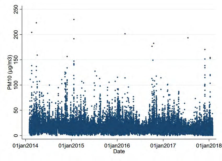
1     Introduction
Transportation is a major contributor to urban air pollution and greenhouse gas
emissions. Despite substantial improvements in the energy efficiency of vehicles, a
long tradition of imposing air quality standards, and increased attention towards cli-
mate change mitigation, most countries around the world still struggle with the dual
challenge of poor ambient air quality and high levels of carbon emissions from trans-
portation (WHO, 2016; EEA, 2019).1 While more ambitious policies are needed to
curb emissions, imposing higher costs on driving is often met with substantial public
opposition, where critics point to unfavorable distributional properties of such poli-
cies. Previous studies also show that regulations aimed at mitigating air pollution
and other driving-related externalites can have unintended consequences (Davis,
2008; Auffhammer and Kellogg, 2011; Bento et al., 2014; Gibson and Carnovale,
2015), sometimes even leading to net welfare losses. Unintended consequences may
arise due to drivers’ substitution behavior, or by exploitation of policy loopholes.
Understanding the impacts of transportation policies aimed at mitigating local and
global externalities, as well as their distributional implications, is hence crucial in
order to facilitate an efficient and equitable low-carbon transition in the transporta-
tion sector.
    In this paper, we combine highly detailed data on air pollution, traffic, and car
ownership to shed light on efficiency and equity impacts of a congestion charge that
increased the costs of driving gasoline and diesel vehicles during rush hours. While
command-and-control type of regulations such as low-emission zones and license
plate-based driving restrictions are often used to combat urban air pollution, with
mixed success (Davis, 2008; Wolff, 2014; Zhang et al., 2017; Zhai and Wolff, 2020),
market-based policies such as congestion charging have recently been implemented
in several major cities around the world (e.g., Stockholm, Zürich, Milan, London,
Singapore). Still, there are few empirical studies exploiting quasi-experimental vari-
ation to estimate effects of these types of policies on travel behavior and emissions.2
Are these types of market-based polices able to mitigate air pollution and induce a
shift towards greener modes of transportation? Or are drivers simply substituting
towards lower priced hours or roads, potentially leaving the total traffic volume un-
changed? What are the distributional consequences of increasing the price of driving
a high-emission vehicle, and to what extent are low-income households able to adapt
   1
     According to the World Health Organization (WHO), over 90% of the world’s population live
in places where air quality levels exceeds the health-based guidelines (WHO, 2016).
   2
     Notable exceptions include e.g., Gibson and Carnovale (2015) and Simeonova et al. (2019). A
more comprehensive literature review is provided towards the end of the introduction.

                                               1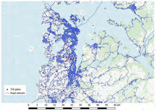
by adopting costly electric vehicles exempted from congestion charging?
    To examine these issues, we exploit a congestion charge implemented in 2016
in the second largest city in Norway (Bergen) that raised the price of entering the
city center toll cordon during rush hours by 80 %. The congestion charge only
applied to weekdays, and only to gasoline and diesel vehicles. While the main goal
of congestion charging is usually to lower traffic volumes during rush hours, the
Bergen congestion charge was to a large extent motivated by an aim of improving
air quality and to speed up the adoption of battery-electric vehicles (electric vehicles
in the following), which have been exempted from paying congestion charges and
road toll in Norway since 1997.3 The policy hence increased the relative price of
driving a high- vs. low-emission vehicle. Before 2010, access to high-quality electric
vehicles were limited, and polices favoring these cars likely had a modest impact
on adoption. However, with the roll-out of several high quality models over the
past decade, electric vehicles have become a feasible option, thereby expanding the
opportunity set of drivers (Figenbaum et al., 2015). Given the exceptionally high
market penetration of electric vehicles in Norway, the Bergen congestion charge
makes for an interesting study case to examine the margins of adjustment when
drivers face a time-of-day and vehicle-specific charge on driving.4
    As a first step, we examine the overall effect of the congestion charge on traffic
volume and ambient air quality using high-frequency sensor and monitoring station
level data. To identify causal effects of the policy, we exploit two sources of variation
across time: pre and post policy and weekday vs. weekend.5 Results from the
empirical examination show a negative and significant effect on both traffic volume
and air pollution; increasing the rush hour rate of entering the toll cordon by around
80 % led to a 14 % decrease in cars entering the congestion zone during rush hours
and an 11 % reduction in concentrations of NO2 during midday hours.6 While we
find evidence of inter-temporal substitution towards the 15-30 minutes right before
and after rush hours, as well as spatial substitution towards lower priced roads,
the overall change in traffic is dominated by the large reductions on treated roads
during rush hours. These findings suggest that drivers primarily substituted towards
other modes of transportation. Averaging effects over the course of a day, we find
   3
     From 2019 and onward the policy was changed, and electric vehicles were charged with ∼20
percent of the standard rate. This policy change, however, is outside the time frame of our dataset.
   4
     In the first quarter of 2019, over 50% of all new passenger vehicles sold in Norway were electric
vehicles; see elbil.no. In the year of the congestion charge implementation (2016), the share of
electric vehicles of all new passenger vehicles sold in Norway was around 16%.
   5
     The congestion charge was only active during weekdays.
   6
     We find similar sized effects for NO2 when applying a difference-in-differences specification
that exploits variation across cities instead of weekday vs. weekend. A similar specification is not
feasible for traffic volumes due to lack of comparable data across cities.

                                                  2
that daily traffic volume on rush-hour priced roads decreased by around 4.8 % and
ambient levels of NO2 decreased by 6.5 % (or 3.1 µg/m3 ). We find a similar-sized
percentage decline in PM10 , but estimates are too noisy to draw firm conclusions.
As PM10 is largely generated from wear and tear from roads, tires and break blocks
rather than vehicle exhaust, a change in fleet composition towards electric vehicles
is likely to lower NO2 concentrations but not necessarily PM10 .
     To further examine behavioral responses to the congestion charge, we exploit a
novel data set that combines registry data on the full population of cars in Norway
with detailed socioeconomic information on households, including the neighborhood-
level location of individuals’ home and workplace. Combining this exceptionally
detailed data with information on the road network and the location of toll gates,
we are able to identify the toll payments faced by each individual household when
traveling between home and work – provided that they choose the shortest route.
Based on these datasets, we construct treatment and control groups in a triple
differences framework. Specifically, we define the treatment group as households
exposed to congestion charging on their way to work and the control group as
households where the work route does not have toll gates.7 We then compare the
treatment and control groups pre and post policy and across two similar-sized cities
in Norway (Bergen and Stavanger), where Stavanger serves as the “placebo” case.
By comparing the development of similar types of households across two cities, we
are able to control for differential, time-varying effects of the increased availability
of electric vehicles on households that pay and do not pay road toll. Identification
is further strengthened by the inclusion of neighborhood-year level fixed effects,
household level demographics and travel time between home and work with both
car and public transit.
     Results from the empirical examination suggest that households respond to the
congestion charge by substituting towards electric vehicles. We find that households
exposed to the Bergen congestion charge were around 4.2 percentage points more
likely to adopt an electric vehicle. This estimated treatment effect explains around
1/3 of the increase in electric vehicle adoption in the treatment group from 2014
to 2017.8 Further, we find that the positive effect on electric vehicle adoption is
mirrored by a negative effect on the adoption of gasoline and diesel vehicles, leading
to a close to zero effect on the total number of cars owned by a household. This
   7
     This definition serves as a proxy for the overall costs faced by households from congestion
charging.
   8
     From the end of 2014 to the end of 2017, the share of toll-paying commuters in Bergen that
owned an electric vehicle increased by 13 percentage points, from 4.7 percent to 17.7 percent. In
the absence of the congestion charge, we predict that the electric vehicle share in 2017 would have
been 13.5 percent.

                                                3
suggests that households, on average, replaced their fossil fuel car by an electric one.
    Examining heterogeneous effects, we find strong gradients along several socioeco-
nomic dimensions. While the policy had no effect on electric vehicle adoption among
households in the lowest income quintile, the electric vehicle share for households in
the highest income quintile increased by around 7 percentage points as a consequence
of the policy. We also find that treatment effects are larger for university-educated
couples with kids, and for households with a longer work commute and poor public
transit quality. The latter implies that the quality of transportation substitutes
plays a key role in households’ adaptation responses. While the heterogeneous ef-
fects may be explained by differences in preferences, parts may be due to financial
constraints in purchasing an electric vehicle.
    Overall, our findings on car ownership suggest that congestion charging combined
with exemptions for electric vehicles can be a powerful tool to promote electric
vehicle adoption, but that there are systematic differences in how households respond
to the policy. Back-of-the-envelope welfare calculations suggest that the policy led
to a net welfare gain with a benefit to cost ratio of around 3:1.
    The magnitude of our treatment estimates must be seen in context of Norway’s
other existing electric vehicle incentives, such as exemptions from purchasing tax and
value-added tax. These strong financial incentives have contributed to an exception-
ally high market share of electric vehicles in Norway and a relatively well-developed
charging infrastructure. In absence of these favorable conditions, we would likely
have seen a lower effect of the congestion charge on electric vehicle adoption. De-
spite the specific features of our research context, we argue that our findings may
help shed light on expected impacts of congestion charging in other countries in a
future scenario where electric vehicles are more competitive to internal combustion
engine vehicles, e.g. due to policies or technological improvements, and the charging
infrastructure more developed than today.
    Our paper complements the empirical literature on the effects of transportation
polices on air pollution, congestion, and other driving-related externalities. Previous
studies have shown that e.g., low emission zones, road tolls and congestion charges
can help improve urban air quality (Wolff, 2014; Gibson and Carnovale, 2015; Fu
and Gu, 2017; Gehrsitz, 2017; Simeonova et al., 2019; Pestel and Wozny, 2019; Zhai
and Wolff, 2020), with resulting health benefits such as lower asthma rates in chil-
dren (Simeonova et al., 2019), lower infant mortality (Currie and Walker, 2011),
and fewer hospital admissions related to chronic cardiovascular and respiratory dis-
eases (Pestel and Wozny, 2019). While these studies provide important estimates
on environmental and health effects of transportation policies, very few studies com-

                                           4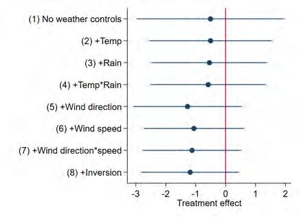
bine highly detailed data with a quasi-experimental design to examine underlying
mechanisms through which individuals respond to these policies, as well as how
these mechanisms differ across households. The majority of papers also focus on
command-and-control instruments; by contrast we provide estimates on the effects
of a marked-based policy implemented in several major cities over the past decade.
    Our paper also contributes to a small but growing quasi-experimental literature
on electric vehicle adoption. Existing studies focus on the effects of purchasing
subsidies (Muehlegger and Rapson, 2018; Clinton and Steinberg, 2019), charging
infrastructure (Li et al., 2017) and low emission zones (Wolff, 2014) on new vehicle
registrations, usually at the zip-code, metropolitan, or state level. By contrast, we
examine effects of a congestion charge paired with electric vehicle exemptions on
household-level car ownership. Compared to previous studies, we use exceptionally
detailed data, were we are able to locate the residence and workplace of each indi-
vidual living in Norway. This allows us to construct a policy exposure measure that
vary substantially across space and time, which helps to develop a more credible
identification strategy. Further, by using data on households’ car portfolio rather
than just new car sales, we are able to examine whether the policy increased or
decreased the total number of cars – a crucial aspect to understand the net environ-
mental and climate benefits of electric vehicle incentives.
    The remainder of the paper is organized as follows: Section 2 provides back-
ground information on the policy and the broader institutional setting. Section 3
describes the data and results for pollution and traffic. Section 4 describes data and
results for household-level transportation behavior. Section 5 provides a discussion
of the net welfare effects and distributional concerns. Section 6 concludes.

2    Background
The congestion charge in Bergen was announced in February 2015 and implemented
one year later, on February 1st 2016; see Table 1. The congestion charge was
electronically collected via the existing automated toll gates in and around the city
center of Bergen; see Figure 1. Before implementation, small passenger vehicles
passing the toll cordon paid an amount of NOK 25 (∼$3) irrespective of time of day.
After the introduction of congestion pricing, small passenger vehicles faced a rush-
hour rate of NOK 45 (∼$5.4) in the hours 06:30-09:00 and 14:30-16:30, equivalent
to an 80 % price increase. The rush hour rates were only active on weekdays.
Rates in non-rush hours were lowered to NOK 19 (∼$2.3), representing a 24 % price
decrease. Vehicles were charged when entering the toll cordon. If a vehicle passed

                                          5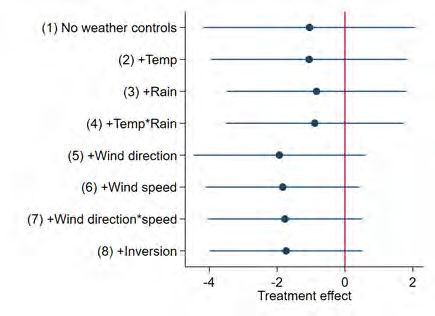
Table 1: Congestion charging in the city of Bergen

                    Date implemented                                 Feb 1, 2016
                    Date announced                                   Feb 18, 2015
                    Morning rush                                     06:30-09:00
                    Afternoon rush                                   14:30-16:30
                    Price pre Feb 1, 2016             NOK 25 (∼$3)
                    Price post Feb 1, 2016: rush hour NOK 45 (∼$5.4)
                    Price post Feb 1, 2016: non-rush NOK 19 (∼$2.3)
                 Notes: Rates are given in NOK. 10 NOK ≈ 1 EUR and ≈ 1.2 USD. Rates
                 correspond to the levels at the time of implementation and reflect rates faced
                 by small passenger vehicles (< 3500 kg) . For large vehicles (> 3500 kg)
                 the price was 50 NOK before Feb 1st 2016, and 90 NOK during rush hours
                 (38 NOK outside rush hours) after policy implementation. Battery electric
                 vehicles were exempted from the congestion charge and toll rates throughout
                 the period analyzed. Hybrid electric vehicles were subject to the same rates
                 as internal combustion engine vehicles (ICEVs). Appendix Figure A.3 shows
                 the development of toll rates in Bergen over the period 2005 to 2017.

the toll cordon several times within an hour, it was only charged once.9 Battery-
electric vehicles were exempted from toll rates both before and after the introduction
of the congestion charge. The congestion charge hence further increased the relative
cost of driving a diesel or gasoline vehicle compared to a battery-electric vehicle.10
    While the main goal of rush hour pricing is usually to mitigate congestion, the
introduction of the Bergen congestion charge was to a large extent motivated by
air quality concerns. In the years leading up to implementation, Bergen together
with a handful of larger cities in Norway struggled with poor urban air quality, and
in 2015 Norway was convicted in the EFTA court for violating EU’s ambient air
quality standards in several parts of the country.11 The majority of the violations
were linked to excess concentrations of NO2 in urban areas, where exhaust from road
traffic is usually a major source; see Section 3.1 for details. As a consequence of the
court decision, Norway was required to initiate measures to meet the requirements
of the EU Air Quality Directive.
    Beyond meeting air quality requirements, the introduction of the congestion
charge was also seen as an instrument to lower CO2 emissions and facilitate the shift
towards greener modes of transportation. As almost 98 % of Norway’s electricity
   9
     There was also a monthly cap on the overall cost per vehicle. Once the cap was reached, the
vehicle was allowed to enter the toll cordon free of charge. However, this cap was set too high to
be binding for regular commuters.
  10
     See e.g., NPRA (2018) for more details on the policy, and for a descriptive analysis of traffic
volumes after the introduction of the policy. Congestion charging has also been implemented in four
other cities in Norway; see Appendix Table A.1. In this paper, we focus on the Bergen congestion
charge as we either lack sufficient air pollution data on the other cities, or lack information on car
ownership for the post period.
  11
     See e.g., regjeringen.no and nrk.no.

                                                       6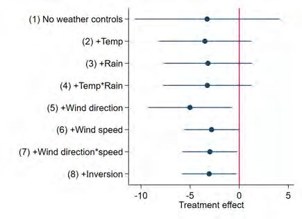
Figure 1: Map of toll gates, pollution monitoring stations and weather stations in
Bergen

                                                                 Danmarks plass

     Toll stations
     Weather stations
     Pollution stations
     Road network
  Notes: The map shows toll gates, weather stations, and pollution monitoring stations in and around the city
  centre of Bergen. The only pollution monitoring station with a sufficiently long time series to use in the
  analysis is the monitoring station labeled as Danmarks plass. See Appendix A for additional maps of Bergen
  and the road network.

production is renewable (Statistics Norway, 2020), electric vehicles cause very low
indirect CO2 emissions from driving. Norway has an ambitious goal of increasing
the market share of electric vehicles to 100 % by 2025 (NTP, 2017, p. 224), and the
congestion charge exemption was one of many benefits granted to electric vehicle
owners over the time period analyzed. At the national level, electric vehicles are
exempted from purchase taxes and VAT. At the local level, electric vehicles benefit
from exemptions from road toll and congestion charges, access to bus lanes, free
parking, and free charging. See Appendix Table A.3 for a complete list of electric
vehicle incentives.
    The strong incentives have contributed to an exceptionally high market share of
electric vehicles in Norway - the highest in the world in 2017 (IEA, 2018). The high
share has been facilitated by a dramatic increase in the supply of electric vehicle
models since 2010.12 While many of the policies promoting electric vehicles have
been in place since the 1990s, their impact likely increased as several high-quality
 12
    See Figenbaum et al. (2015) for an overview of electric vehicles introduced in the Norwegian
market.

                                                      7
electric vehicle models became available. When estimating effects of the congestion
charge on individual-level behavior, it will therefore be important to control for the
potentially differential time trends across households with different levels of exposure
to electric vehicle benefits. For instance, households paying road toll on their way
to work will have a stronger incentive to adopt an electric vehicle, and the response
is likely to increase as more electric vehicles become available - also in the absence
of an increase in road toll. In this paper, we aim to disentangle the effect of the
Bergen congestion charge from other policy and technology trends by constructing
a control group that faced similar local and national policies and incentives - with
the exception of congestion charging.
The introduction of congestion charges in Norway has sparked a lot of public
discontent, where critics often point to unfavorable distributional properties of the
policy. As all drivers face the same rate, those from lower-income households will
necessarily spend a larger share of their overall budget if similarly exposed to the
congestion charge. Critics have also pointed to the lack of high-quality substitutes
for many households, locking them into existing behavioral patterns. Purchasing
a battery-electric vehicle to avoid road toll and congestion charges is still out of
reach for many households – despite the large tax exemptions. In the spring and
summer of 2019, there were several mass protests around the country against higher
toll rates and congestion charging, which resulted in the formation of a new, single-
cause political party pledging to remove all toll gates. The new “road toll party” got
a substantial share of the votes in the local elections in the fall of 2019, leading to the
cancellation of planned congestion charges and new toll gates.13 Despite claims of
the policy disproportionately harming low-income households, there is little evidence
on how individuals actually adapted to the policy and to what extent they seemed
to be locked into behavioral patterns due to e.g., income and limited public transit
options.
3 Part I: air pollution and traffic volume
What was the effect of the congestion charge on rush hour and daily traffic? And
to what extent did the policy improve ambient air quality? In the following, we
examine these questions using high-frequency data from traffic sensors and pollution
monitoring stations.
13
See e.g. https://www.nrk.no/osloogviken/bomringen-i-drammen-skrotes-1.14560632
(accessed September 11, 2020; Norwegian only).
83.1 Data and descriptives
3.1.1 Traffic volume
To investigate effects of the congestion charge on traffic, we collect sensor level
data on traffic volume and composition from the local road toll company in Bergen
(Ferde). A map of the 14 automated toll gates, which indicate the congestion
charging area, is provided in Figure 1. The sensor level data contains information
on all cars passing the automated toll road gates in the period 2014 to 2018, with a
15-minute resolution. The number of cars within each 15 minute interval is further
split into vehicles weighing less than 3.5 tonnes (referred to as “passenger vehicles”)
and vehicles weighing 3.5 tonnes or more (refereed to as “trucks”).14 In the main
analysis, we focus on the total number of cars passing any toll gate in or out of
Bergen in a given time period. By aggregating traffic to the city level, we eliminate
the toll gate dimension of the data and are left with a high-frequency time series
of total traffic.15 Further, we focus on a period covering two years before and two
years after the congestion charge was implemented, i.e., Feb 1 2014 to Feb 1 2018.
This ensures that toll rates were constant in the pre-treatment period; see Appendix
Figure A.3.
Figure 2: Traffic volume two years before and after Feb 1 2016
(a) Weekday (b) Weekend
4000 4000
3000 3000
All cars/15 min
All cars/15 min
2000 2000
1000 1000
0 0
0 2 4 6 8 10 12 14 16 18 20 22 24 0 2 4 6 8 10 12 14 16 18 20 22 24
Time of day Time of day
Post (+730 days) Pre (-730 days) Post (+730 days) Pre (-730 days)
Notes: Figures show the average number of vehicles passing the toll cordon over the course of a day based
on 15 minute intervals. Panel (a) shows averages for weekdays (Monday-Friday) and panel (b) shows averages
for the weekend (Saturday-Sunday). Dashed lines indicate averages for the 730 days (2 years) prior to policy
implementation. Solid lines indicate averages for the 730 days (2 years) post policy implementation. Gray shaded
areas indicate rush hours (06:30-09:00 and 14:30-16:30). Note that the congestion charge was not active during
weekends. See Appendix Figure B.1 for traffic volume presented separately for passenger vehicles and trucks. See
Appendix Figure B.2 for similar figures using a period of 365 days pre/post policy implementation. See Appendix
Figure B.3 for traffic volume 365 days pre and post Feb 1 2015 (“placebo intervention”).
14
Note that vehicles weighing less than 3.5 tonnes also consist of taxis, vans, and service vehicles.
Vehicles weighing 3.5 tonnes or more also consist of buses and emergency vehicles in addition to
trucks.
15
Main results are not sensitive to the level of aggregation, as shown in Appendix B.2.3.
9Figure 2 shows how vehicles passing the toll gates are distributed over the course
of a day two years before (dashed line) and two years after (solid line) the conges-
tion charge was implemented. Panel (a) clearly indicates that traffic volumes peak
around rush hours, and that rush hour traffic declined in the two years after policy
implementation.16 The figure also shows a small increase in the number of cars
right before and after rush hours, suggesting that the policy induced some drivers to
change their departure time to avoid the increased cost. However, this substitution
towards non-rush hours seems to be limited to a 15 minute interval before and after
rush hours. The traffic pattern during weekends, when the congestion charge was
not active, looks very similar in the two years before and after the policy; see panel
(b) in Figure 2.17
3.1.2 Air pollution
To examine effects of the policy on ambient air quality, we collect hourly data on
atmospheric pollution for the period 2014-2018 from the Norwegian Institute for
Air Research (NILU), which operates a number of air monitors across Norway. Air
pollution is measured as micrograms per cubic meter of air (µg/m3 ). Figure 1 shows
a map with the location of monitoring stations in the inner city of Bergen. While
there are several monitoring stations located within the congestion zone, only one
monitoring station has a sufficiently long time series to examine effects on the policy
(the station labeled Danmarks plass). We hence limit the analysis to this station
only when estimating effects on air pollution.
In the analysis, we focus one two key air pollutants: nitrogen dioxides (NO2 )
and particulate matter with a diameter between 2.5 and 10 micrometers (PM10 ).18
NO2 is one of a group of highly reactive gases known as nitrogen oxides (NOx ).
The most important source of NO2 in Norway is exhaust from vehicles with an
internal combustion engine, i.e., gasoline and diesel vehicles (NILU, 2019).19 High
ambient levels of NO2 is usually an urban phenomenon, and in the period analyzed
several of the larges cities in Norway violated the national air quality standards
for NO2 . Epidemiological studies have documented several adverse health effects of
exposure to NO2 , such as aggravation of asthma and bronchitis, impaired respiratory
functions, and mortality (see e.g., Lipsett et al., 1997; Shima and Adachi, 2000).
16
The reduced traffic during rush hours are primarily driven by passenger vehicles; see Appendix
Figure B.1.
17
See Appendix B.1 for additional descriptives.
18
These are the two pollutants most relevant to road traffic, and are also the ones where we
have sufficient data to perform the analysis. An overview of the relative contribution of different
sources to six different air pollutants is provided in Appendix Table A.2.
19
Other less important sources of NO2 are manufacturing industry and ship traffic.
10Recent studies also suggest that NO2 have adverse health effects also for ambient
levels well below national ambient air quality standards (Simeonova et al., 2019;
Breivik et al., 2020).
Particulate matter is a mixture of solid particles and liquid droplets such as
dust, dirt, soot, or smoke. PM is usually divided into two categories according to
the size of the particles. PM10 refers to particles with diameters between 10 and
2.5 micrometers.20 The most important sources of PM10 in urban areas in Norway
are wear and tear from roads, car tires and break blocks, sand added to roads to
increase friction of icy surfaces in the winter, and wood-fired ovens (NILU, 2019).
The epidemiological literature has documented several adverse health effects from
exposure to PM10 and PM2.5 , such as premature death in people with heart and
lung disease, aggravated asthma, and decreased lung growth and lung function in
children (see e.g., Avol et al., 2001).
Figure 3 shows how ambient levels of NO2 and PM10 vary over the course of 24
hours in the two years before (dashed line) and after (solid line) policy implemen-
tation. Gray shaded areas indicate rush hours. Both pollutants show a peak during
the weekday morning rush, with a more pronounced peak for NO2 . By comparing
the average pollution levels pre and post policy, we see that there is a clear decline
in ambient air pollution on both weekdays and weekends. However, the decline in
µg/m3 seems to be largest for weekdays.21 To put the levels of air pollution into
context, the WHO Air Quality Guidelines for NO2 and PM10 are 40 µg/m3 annual
mean and 20 µg/m3 annual mean, respectively (WHO, 2006). See Appendix C.1 for
additional descriptives and summary statistics.
3.1.3 Weather
To control for the effects of weather on traffic and pollution outcomes, we col-
lect monitor-level weather data from the Norwegian Meteorological Institute for the
years 2014-2018. We focus on hourly measures of temperature, precipitation, wind
speed, and wind direction. The weather data is linked to a pollution monitoring
station by calculating the inverse distance weighted average of observations from all
weather stations within a 50 kilometer radius of a pollution monitoring site. Based
on hourly wind data, we construct four wind direction categories.22 Additionally,
20
PM2.5 refers to particles with a diameter of 2.5 micrometers or smaller.
21
If we restrict the sample to one year pre and post policy implementation, there appears to be
no reduction in NO2 on weekends and a large reduction on weekdays; see Appendix Figure C.2.
For PM10 there is a similar, but less striking pattern.
22
Categorization is based on wind direction in degrees. Northern ∈ [0-45] and (315,360], Eastern
∈ (45,135], Southern ∈ (135,225], Western ∈ (225,315].
11Figure 3: Air pollution two years before and after Feb 1 2016
(a) Weekday NO2 (b) Weekend NO2
(c) Weekday PM10 (d) Weekend PM10
Notes: Figure shows average ambient air pollution over the course of a day for the pollution monitoring station
located at Danmarksplass in Bergen. Values are based on 60 minute intervals. Panels (a) and (c) show averages for
weekdays (Monday-Friday) and panels (b) and (d) show averages for weekends (Saturday-Sunday). Dashed lines
indicate averages for the two years prior to policy implementation (Feb 1 2016). Solid lines indicate averages for
the two years post policy implementation. Gray shaded areas indicate rush hours. Note that congestion charging
is not active during weekends. Pollution is measured as micrograms per cubic meter of air(µg/m3). See Appendix
Figure C.3 for ambient air pollution one year pre and post Feb 1 2015 (”Placebo intervention”). See Appendix
Figure C.2 for similar figures using a period of one year pre and post policy intervention.
we collect data on temperature inversion episodes in Bergen from the Nansen En-
vironmental and Remote Sensing Center.23 The dataset contains temperature for
Bergen recorded at different altitudes, allowing us to identify inversion episodes, i.e.,
periods in which the temperature is increasing in altitude. As cold air is heavier
than warm, air inversion episodes tend to reduce air circulation close to the surface
and thus trap the pollutants produced by vehicles (and other sources) close to the
ground. In the 2 years pre and post policy, inversion episodes occurred for around
4 % of the hourly observations; see Appendix C.1.
23
The data is available from the following website: https://veret.gfi.uib.no/?action=
download.
123.2 Empirical strategy
In this subsection, we provide an empirical framework to help estimate a causal effect
of the congestion charge on traffic volume and air pollution. While the descriptive
evidence presented in Section 3.1 suggest a decline in traffic and air pollution after
the introduction of the congestion charge, the reduction might have been due to
other factors than the policy, such as weather conditions, the use of wood-fired ovens,
road construction, the supply of low and zero emission vehicles, etc. To identify the
causal (short-run) effect of the policy, we employ a differences-in-differences (DiD)
framework, where we exploit the fact that rush hour charges were not active during
weekends.24 By defining weekdays as our treatment observations and weekends as
our control observations, we mitigate the risk of estimates being confounded by other
factors that change over time and affect traffic or pollution simultaneously. The
key identifying assumption is that changes in omitted time-varying variables, such
as unobserved technological trends, economic activity and local policy initiatives,
affect weekday and weekend traffic and air pollution similarly.
Our main regression equation can be written as:
yikt = βpostt × weekdayt + Xit0 γ + λym + θdi + εikt , (1)
where yikt denotes the outcome of type k observed at time interval i on date t; Xit0 is
a vector of weather controls; λym denotes year×month fixed effects; θdi denotes day-
of-week×time-of-day fixed effects; and εikt is the idiosyncratic error term. Finally,
postt is a dummy variable equal to 1 after February 1st 2016, and weekdayt is a
dummy variable equal to 1 during weekdays, meaning that β is the coefficient of
interest. Seasonal variation and long-term time trends are absorbed by λym , while
pre-policy weekday-weekend differences are absorbed by θdi . Thus, the variation left
to identify β̂ is the pre-post difference between weekdays and weekends. In the main
specifications standard errors are clustered at the weekly level.
For the main traffic regressions, yikt denotes the total traffic volume of type
k ∈ {all vehicles, passenger vehicles, trucks} passing the toll cordon in Bergen dur-
ing a 15 minute interval. For air pollution regressions, yikt denotes the concentration
of pollutant k ∈ {NO2 , PM10 } measured at hourly intervals. Both regression spec-
ifications include the same vector of weather controls.25 Our main specification is
24
Looking at Figure 2, panel (b) it does not seem like the traffic pattern during weekends changed
visibly pre vs. post policy implementation.
25
While weather controls are arguably more important in the air pollution regressions, weather
conditions may also affect traffic volume. For consistency reasons, we use the same vector of
weather controls in both regressions: three polynomials of air temperature; two polynomials of
precipitation; the interaction of temperature and precipitation; two polynomials of wind speed;
13based on a sample consisting of 730 days (two years) before and after the policy
implementation. This is the longest time interval our data allows that ensures that
seasonal trends in traffic or pollutants are balanced pre and post. We remove ir-
regular days, such as vacations and summer months. Alternative specifications and
robustness checks are provided in Appendix B.2.
We consider our DiD strategy to give us a conservative treatment estimate, for
at least two reasons. First, as some pollutants can stay in the air for several hours
(depending on weather conditions among other factors), a policy-induced reduction
in weekday pollution may lower ambient levels of air pollution on weekends as well.
In the presence of such positive spillovers from weekdays to the weekend, we expect
our DiD strategy to downward bias treatment effects. Second, if the policy leads
to behavioral changes that are carried over to weekends, our treatment estimate
will difference out these effects. For instance, one might suspect that the policy
led to more cycling, walking and use of public transit, and that individuals that got
accustomed to these modes of transportation were also more inclined to change their
behavior during weekends. Furthermore, if households bought electric vehicles as
a response to the policy, they likely also used these vehicles during weekends. Our
DiD estimate should therefore be interpreted as a lower bound on the causal effect
of the policy.26
3.3 Results on traffic volume
Figure 4 displays the estimated treatment effects of the policy, where estimates are
allowed to vary by 15 minute increments. Comparing these 96 different treatment
effects allows us to identify the time intervals with the largest treatment effects,
as well as explicitly examine intertemporal substitution. The figure clearly follows
the same pattern as Figure 2; traffic shows a sharp decline during the morning and
evening rush hours and an increase in the 15-30 minutes before and after rush hours.
In the remaining hours of the day, the effect of the congestion charge on traffic is
close to zero. These findings imply that the policy worked as intended, by inducing
drivers to either change their mode of transportation or substitute towards lower
priced hours. The increase in traffic right before and after rush hours are clearly
dominated by the reduction during rush hours, implying an overall reduction in
daily traffic.
four dummies for wind direction (north, south, east and west) as well as their interaction with
wind speed; and finally, a dummy for inversion episodes. We estimate two sets of each of these
weather control variables; one for weekdays and one for weekends.
26
For air pollution, the data permits us to present an alternative DiD estimate based on differ-
ences across cities and over time; see Appendix C.3 for details.
14Figure 4: DiD estimates on traffic volume by 15 min. intervals. 2 years pre/post
1000
800
600
Change in # of vehicles
400
200
0
-200
-400
-600
-800
-1000
0 2 4 6 8 10 12 14 16 18 20 22 24
Time of day
Notes: Figure plots treatment effects estimated from from equation 1, where regressions are run separately for each
15 minute increment. Whiskers indicate 95% confidence intervals. Standard errors are not adjusted for multiple
hypothesis testing. Gray shaded areas indicate rush hours. Traffic is measured as the total number of cars passing
the toll cordon every 15 minutes. Standard errors are clustered at the week level.
Table 2 shows the average daily treatment effect (column 1), as well as treatment
effects for five different time periods of the day (columns 2-6). Overall, the congestion
charge led to a 4.8 % reduction in daily traffic volume during weekdays (around 78
vehicles per 15 minute interval, or 7,456 vehicles per day).27 Note that this estimated
effect incorporates intertemporal spillovers within a day. Columns (2)-(4) indicate
that traffic during rush hours was significantly reduced by 14.4 % (around 447
vehicles per 15 minute interval). Column (5) shows a 9 % increase in traffic in the
30 minutes before and after the morning and evening rush, indicating intertemporal
substitution. Column (6) shows a small reduction in traffic during other non-rush
hours (1.3 %) that is significant at the 10 % level.28 See Appendix Table B.1 for
results split by passenger vehicles and trucks.
To illustrate the magnitude of the intertemporal substitution, we translate the
15 minute effects to the total increase or decrease in the number of vehicles within a
given time period. While rush hour traffic decreased by (447×18 quarters =) 8,046
cars, there was an increase of (207.8×8 quarters =) 1,662 cars in the 30 minutes
27
77.67 cars per quarter × 96 quarters per day = 7,456 cars per day.
28
This might be related to the small reduction in fees outside rush hours. However, the reduction
in fees outside rush hours also applies to weekends, and will therefore to some degree be differenced
out. Note, however, that traffic during weekends did not seem to decrease (see Figure 2. Thus, it
seems like the reduction in fees outside rush hours had limited impact on overall traffic volume.
15Table 2: DiD estimates on traffic volume. 2 years pre/post
Rush hours Non-rush hours
Dependent variable: All day All Morning Evening +/-30 min Other
# vehicles/15 minute interval (1) (2) (3) (4) (5) (6)
Post × weekday -77.67∗∗∗ -447.0∗∗∗ -445.7∗∗∗ -436.9∗∗∗ 207.8∗∗∗ -15.42∗
(9.889) (23.18) (29.33) (25.68) (19.89) (7.971)
Observations 87518 16416 9122 7294 7294 63808
Mean depvar (pre, weekday) 1632 3104 3239 2936 2316 1175
Change (%) -4.76 -14.40 -13.76 -14.88 8.97 -1.31
Weather controls (Xit0 γ ) X X X X X X
Month × year FE (λym ) X X X X X X
Day-of-week × time-of-day FE (θdi ) X X X X X X
Notes: Table shows results from 6 separate regressions. Dependent variable is vehicles passing toll gates in Bergen
during a 15 minute interval. Post×weekday refers to the β coefficient estimated from Equation 1. Column headings
indicate the sample used in each regression. “Rush hours” refer to the intervals 06:30-08:59 (morning) and 14:30-
16:29 (evening). For non-rush hours, “+/- 30 min” refers to the 30 minute intervals right before and after rush
hours. “Other” refers to the remaining non-rush hours (i.e., 9:30-13:59 and 17:00-05:59). Sample is restricted to
730 days pre and post policy implementation. Standard errors clustered at the weekly level in parentheses. *
pour data does not allow us to examine whether the deterred trips are not taking
place at all, or whether people are substituting towards other modes of transport
such as public transit, walking, cycling or car pooling.
3.4 Results on air pollution
Figure 5 shows hourly DiD estimates for NO2 and PM10 . From Figure 5 panel (a),
we see that the congestion charge led to significant reductions in NO2 most hours
between 6 am and 5 pm. The largest reductions occur in the time period right after
the morning rush. As air pollutants can stay in the air for a period of time after they
are released, we do not expect to see the same sharp differences between rush hours
and non-rush hours as in Figure 2.31 If we compare the estimated treatment effects
to the raw means presented in Figure 3, the estimated effects are very similar to
the observed difference in NO2 concentrations before and after the policy, indicating
that most of the change in NO2 over time can be attributed to the congestion charge.
Figure 5: DID estimates on NO2 and PM10 by 60 min. intervals. 2 years pre/post
(a) NO2 (b) PM10
Notes: Figure plots the coefficient β estimated from Equation 1. Each coefficient reflects the estimated treatment
effect from a separate regression, where the sample is restricted to the 1 hour interval indicated on the x-axis.
Sample period is restricted to 2 years before and 2 years after policy implementation (Feb 1 2016). Gray shaded
areas indicate rush hours. Pollution is measured as micrograms per cubic meter of air (µg/m3 ). See Appendix
Figure C.4 for results based on a sample restricted to 1 year before and after policy intervention. See Appendix
Figure C.6 for ”placebo” estimates based on 1 year before and after Feb 1 2015.
Table 3, panel (a) shows average daily treatment effects for NO2 (column 1)
together with average treatment effects for 5 different time intervals (columns 2-6).
The coefficient in column (1) suggests that the congestion charge lowered NO2 con-
centrations by 3.1 µg/m3 on average during a day, corresponding to a 7 % reduction.
The effect is driven by reductions during and between rush hours; NO2 concentra-
tions were 6.8 µg/m3 lower during rush hours, corresponding to a 11 % reduction,
31
The length of the period air pollutants stay in the air will vary with weather conditions, such
as precipitation, wind speed and inversion episodes.
17while estimated effects on NO2 during the evening and night time are close to zero
and insignificant.32
Table 3: DID estimates on NO2 and PM10 . 2 years pre/post
24 hours Daytime Midday Rush Evening Night
Dependent variable: 00-23 05-22 06-17 6-9,14-16 18-23 00-05
ambient air pollution (µg/m3) (1) (2) (3) (4) (5) (6)
Panel A: NO2
Post × weekday -3.064∗∗ -4.334∗∗∗ -6.719∗∗∗ -6.813∗∗∗ -0.182 0.323
(1.369) (1.576) (1.634) (1.658) (1.915) (1.300)
Observations 21438 16041 10637 6227 5403 5398
Mean depvar (pre-weekday) 47.01 55.06 60.86 63.78 42.30 24.58
Change (%) -6.52 -7.87 -11.04 -10.68 -0.43 1.32
Panel B: PM10
Post × weekday -1.185 -1.690∗ -2.084∗ -1.735 -0.868 0.565
(0.809) (0.955) (1.163) (1.115) (0.850) (0.699)
Observations 21624 16219 10794 6314 5429 5401
Mean depvar (pre-weekday) 18.81 21.02 22.29 21.76 18.67 12.01
Change (%) -6.30 -8.04 -9.35 -7.97 -4.65 4.70
Weather controls (Xit0 γ) X X X X X X
Month×year FE (λym ) X X X X X X
Day of week×time-of-day FE (θdi ) X X X X X X
Notes: Table shows results from 12 separate regressions. Dependent variable is ambient air pollution measured
as mean levels of NO2 or PM10 (µg/m3) during a 60 minute interval. Post×weekday refers to the coefficient β
estimated from equation 1. Column headings indicate the sample used in each regression. Rush hours refer to the
intervals 06:00-09:59 (morning) and 14:00-16:59 (evening). Sample is restricted to two years pre and post policy
implementation. Standard errors clustered at the weekly level in parentheses. * pcharging on concentrations of NO2 is robust to: (i) trimming the sample to one year
pre and post policy, (ii) using different levels of fixed effects, (iii) using different
combinations of weather controls, and (iv) performing placebo tests using Feb 1
2015 as the intervention date. The same robustness checks also confirm a negative
but non-significant effect on PM10 .
As discussed in Section 3.2, our treatment estimates on NO2 and PM10 should
be interpreted as lower bound estimates of the true effect of the policy. One reason
for this is that we are differencing out effects of changes in travel habits if these spill
over to weekends, such as a shift from driving to cycling. Further, as we will show
in Section 4, the congestion charge led to an increased adoption of electric vehicles,
which may have lead to a higher share of electric vehicles on the road during both
weekdays and weekends.
In an attempt to incorporate these types of behavioral shifts in our treatment
estimate, we present findings from an alternative DiD strategy where we compare
air pollution levels across cities, pre and post the policy. A similar strategy has
been used in previous empirical papers examining effects of various transportation
policies on air pollution (see e.g., Simeonova et al., 2019; Zhai and Wolff, 2020). Note
however that exploiting differences across cities is only feasible for air pollution and
not traffic volume, as we only have access to traffic data from toll gates in Bergen. By
contrast, air pollution readings are available for several cities around the country.
By focusing on weekdays only and using differences across cities, we circumvent
potential problems of spillovers between weekdays and weekends. At the same time,
different cities may be subject to different local policies and time trends that might
confound the treatment effect, and that are hard to control for. The key identifying
assumption is that time-varying omitted variables relevant to air pollution affect all
cities similarly. Estimation results from the spatial DiD strategy are presented in
Appendix C.3 and show that the congestion charge lowered concentrations of NO2
by 4 µg/m3 , or 8.4 percentage points, which is 1.9 percentage points larger than the
main results. Again, we find no significant effect on PM10 .
4 Part II: Household-level behavior
In this part of the paper, we further examine effects of the congestion charge by
moving from station and sensor level data to rich registry data on household level
car ownership. The disaggregated data allows us to ask questions such as: How do
different types of households adapt to the congestion charge? To what extent do
households purchase an electric vehicle in response to the policy? Do households
19simply add a new car to their portfolio, or do they switch from ”brown” to ”green”?
By estimating a rich set of socioeconomic gradients, we also aim to unmask potential
behavioral differences in how households adapt to rising driving costs.33
4.1 Data sources
To construct a dataset on car ownership, household demographics, and congestion
charge exposure, we combine data from several sources, which are described below.34
4.1.1 Car ownership
We collect data on the full population of vehicles registered in Norway over the
period 2011-2017 from the National Motor Vehicle register. The register contains
technical vehicle information on each car, such as model and fuel type. From the
register, we also collect information on current and previous owners of each vehicle,
as well as the timing of several acquisition and disposal events, including the first
registration date, date of the previous ownership change, scrapping date and/or de-
registration dates. We restrict our dataset to privately owned passenger vehicles and
vans registered for non-commercial purposes, and stock-sample car owners from the
register at the end of each year (December 31st). Even though cars are registered
at the individual level, we consider car acquisitions a household level decision and
hence focus on households’ car ownership in the analysis. This leaves us with a panel
of car ownership at the household×year level, where each observation is a snapshot
of cars owned at the end of each year. See Appendix D for more information.
Figure 6 displays the annual share of households that owns an electric vehicle.
From December 2011 to December 2017, the share of Norwegian households that
owned an electric vehicle increased from around 0 % to around 4.5 % (dashed line).
The ownership share in 2017 was by far the highest in the world at the time.35
For Bergen municipality, the share of households that owned an electric vehicle by
the end of 2017 was around 8 % (solid line).36 In the empirical analysis, we aim
to disentangle effects of the Bergen congestion charge on electric vehicle ownership
33
Ideally we would also like to examine the effect of the policy on household-level driving. How-
ever, data availability prevents us from investigating this margin of adjustment.
34
See also Fevang et al. (2021) for a detailed description of the different data sources.
35
According to IEA (2018), Norway had the world’s highest number of battery-electric vehicles
and plug-in hybrid as a share of the vehicle stock in 2017 (6.4 %). Only two other countries show
a stock share of 1 % or higher: Netherlands (1.6 %) and Sweden (1.0 %). Battery-electric vehicles
(BEVs) account for around two-thirds of the world’s electric car fleet.
36
Note that the ownership share of electric vehicles is significantly higher in cities than in rural
areas, likely due to e.g., stronger local incentives, better accessibility of charging stations, and
shorter distances.
20Figure 6: Electric vehicle ownership
.08 .06
Electric vehicle share
.02 .04
0
2011 2012 2013 2014 2015 2016 2017
Bergen Norway
Notes: Figure plots the share of households that own a battery electric vehicle on December 31 each year over
the period 2011-2017. The first observation reflects the electric vehicle share on December 31st 2011 and the last
observation reflects the electric vehicle share on December 31st 2017.
from other confounding trends, such as the increased supply of electric vehicles and
national EV policies.
4.1.2 Household characteristics
The car ownership data described above is linked to detailed socioeconomic data
on individuals and households from various Norwegian registers, such as the na-
tional population register and tax records. Specifically, we collect information on
age, gender, number of persons and children in the household, employment and re-
tirement status, income, wealth, education, and ownership of a second home (e.g.,
cabin). The registry data contains information about the location of each household
at the basic statistical unit level – the smallest geographical unit for which we have
micro-data. We refer to these units as “neighborhoods”. There are in total more
than 14,000 neighborhoods in Norway, with an average population of around 400
individuals, or less than 200 households.37 The detailed information on households
allows us to control for several characteristics in the empirical analysis that might
influence car ownership, as well as explore heterogeneous effects of the policy.
4.1.3 Journey to work and associated toll payments
In addition to socioeconomic information on individuals and households, all em-
ployed individuals are matched to their employer, allowing us to identify the place
37
By comparison, there were 426 municipalities and 4,856 zip codes in Norway in 2017.
21You can also read