ISMIP6-based projections of ocean-forced Antarctic Ice Sheet evolution using the Community Ice Sheet Model
←
→
Page content transcription
If your browser does not render page correctly, please read the page content below
The Cryosphere, 15, 633–661, 2021
https://doi.org/10.5194/tc-15-633-2021
© Author(s) 2021. This work is distributed under
the Creative Commons Attribution 4.0 License.

ISMIP6-based projections of ocean-forced Antarctic Ice Sheet
evolution using the Community Ice Sheet Model
William H. Lipscomb1 , Gunter R. Leguy1 , Nicolas C. Jourdain2 , Xylar Asay-Davis3 , Hélène Seroussi4 , and
Sophie Nowicki5,6
1 Climate and Global Dynamics Laboratory, National Center for Atmospheric Research, Boulder, CO, USA
2 Univ. Grenoble Alpes/CNRS/IRD/G-INP, IGE, Grenoble, France
3 Los Alamos National Laboratory, Los Alamos, NM, USA
4 Jet Propulsion Laboratory, California Institute of Technology, Pasadena, CA, USA
5 NASA Goddard Space Flight Center, Greenbelt, MD, USA
6 University at Buffalo, Buffalo, NY, USA

Correspondence: William H. Lipscomb (lipscomb@ucar.edu)

Received: 31 December 2019 – Discussion started: 14 January 2020
Revised: 15 November 2020 – Accepted: 9 December 2020 – Published: 10 February 2021

Abstract. The future retreat rate for marine-based regions        hibits threshold behavior, with modest retreat under many pa-
of the Antarctic Ice Sheet is one of the largest uncertain-       rameter settings but complete collapse under some combina-
ties in sea-level projections. The Ice Sheet Model Intercom-      tions of low basal friction and high thermal forcing anoma-
parison Project for CMIP6 (ISMIP6) aims to improve pro-           lies. Large uncertainties remain, as a result of parameter-
jections and quantify uncertainties by running an ensemble        ized sub-shelf melt rates, simplified treatments of calving and
of ice sheet models with atmosphere and ocean forcing de-         basal friction, and the lack of ice–ocean coupling.
rived from global climate models. Here, the Community Ice
Sheet Model (CISM) is used to run ISMIP6-based projec-
tions of ocean-forced Antarctic Ice Sheet evolution. Using
multiple combinations of sub-ice-shelf melt parameteriza-         1   Introduction
tions and calibrations, CISM is spun up to steady state over
many millennia. During the spin-up, basal friction parame-        The Antarctic Ice Sheet has been losing mass at an increasing
ters and basin-scale thermal forcing corrections are adjusted     rate for the past several decades (Shepherd et al., 2018; Rig-
to optimize agreement with the observed ice thickness. The        not et al., 2019). Much of the ice loss has been driven by in-
model is then run forward for 550 years, from 1950–2500,          creased access of warm Circumpolar Deep Water (CDW) to
applying ocean thermal forcing anomalies from six climate         marine-based parts of the West Antarctic Ice Sheet (WAIS),
models. In all simulations, the ocean forcing triggers long-      likely caused in part by radiatively forced changes in wind
term retreat of the West Antarctic Ice Sheet, especially in the   patterns (Thomas et al., 2004; Jenkins et al., 2010; Rignot
Filchner–Ronne and Ross sectors. Mass loss accelerates late       et al., 2013; Holland et al., 2019; Gudmundsson et al., 2020).
in the 21st century and then rises steadily for several cen-      Paleoclimate records show that the WAIS retreated in past
turies without leveling off. The resulting ocean-forced sea-      climates not much warmer than the present, including the
level rise at year 2500 varies from about 150 to 1300 mm,         last interglacial (Dutton et al., 2015). Many WAIS glaciers
depending on the melt scheme and ocean forcing. Further           lie on reverse-sloping beds (i.e., with the seafloor sloping up-
experiments show relatively high sensitivity to the basal fric-   ward in the direction of ice flow), making these glaciers vul-
tion law, moderate sensitivity to grid resolution and the pre-    nerable to the marine ice sheet instability (MISI; Weertman,
scribed collapse of small ice shelves, and low sensitivity to     1974; Mercer, 1978; Schoof, 2007). Models suggest that ice
the stress-balance approximation. The Amundsen sector ex-         in the Amundsen Sea sector, including Thwaites and Pine Is-
                                                                  land glaciers, may already be in the early stages of collapse

Published by Copernicus Publications on behalf of the European Geosciences Union.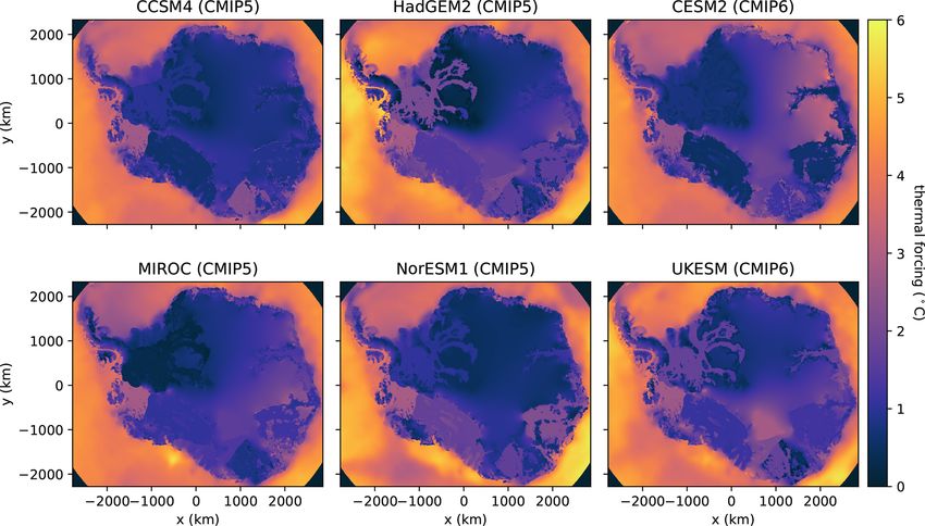
634                                                                     W. H. Lipscomb et al.: CISM Antarctic projections

(Joughin et al., 2014; Favier et al., 2014). Despite recent ad-   2019, 2020). This is not to say that SMB changes are unim-
vances in ice sheet modeling (Pattyn, 2018), projections of       portant for future Antarctic Ice Sheet evolution but rather that
21st century Antarctic Ice Sheet retreat and resulting sea-       the ocean contribution is more uncertain than the SMB con-
level rise (SLR) are highly uncertain, ranging from modest        tribution. Instead, we consider the Antarctic Ice Sheet re-
(∼ 10 cm; Ritz et al., 2015) to large and abrupt (> 1 m; Pol-     sponse to increased sub-ice-shelf melting as a function of
lard and DeConto, 2016). Although recent work (Edwards            basal melting parameterizations (Jourdain et al., 2020) and
et al., 2019) suggests that the most extreme projections may      ESM ocean warming. To study long-term ice sheet evolution,
overestimate the rate of SLR, much of the WAIS is likely          we extend the simulations to the year 2500, with the forcing
vulnerable to long-term, self-sustaining retreat.                 after 2100 based on late-21st-century forcing from high-end
   To improve projections and better understand and               emissions scenarios. In this way, we explore the following
quantify uncertainties, ice sheet modelers have orga-             questions.
nized several community intercomparisons, most re-
cently the Ice Sheet Model Intercomparison Project                  – If the ocean warming projected for the late 21st century
for CMIP6 (http://www.climate-cryosphere.org/wiki/index.              were to continue unabated for several more centuries,
php?title=ISMIP6_wiki_page, last access: 25 January 2021;             what parts of the Antarctic Ice Sheet would be most vul-
Nowicki et al., 2016). ISMIP6 has been endorsed by the                nerable to retreat?
Coupled Model Intercomparison Project – Phase 6 (CMIP6;
Eyring et al., 2016) and is providing process-based ice sheet
                                                                    – Given this vulnerability, and assuming that emissions
and sea-level projections linked to the CMIP ensemble of cli-
                                                                      remain on a high-end trajectory until 2100, what will
mate projections from global climate models. Here, we will
                                                                      be the committed long-term, ocean-forced sea-level rise
refer to these global models as Earth system models (ESMs);
                                                                      from Antarctic ice loss? By “committed”, we refer to
they are also commonly known as atmosphere–ocean general
                                                                      SLR resulting from ice sheet retreat that has been set in
circulation models (AOGCMs). Nowicki et al. (2020) have
                                                                      motion and is likely irreversible.
summarized the ISMIP6 projection protocols for standalone
ice sheet model (ISM) experiments. The general strategy is
to use output from CMIP5 and CMIP6 global models to de-             – How sensitive is the simulated ice sheet retreat to poorly
rive atmosphere and ocean fields for forcing ISMs over the            constrained model parameters and forcing?
period 2015–2100. Goelzer et al. (2020) and Seroussi et al.
(2020) evaluated the multi-model ensembles of projections            Because of modeling and forcing uncertainties that grow
for the Greenland and Antarctic ice sheets, respectively.         larger on timescales beyond a century, our long-term results
   Seroussi et al. (2020) analyzed 16 sets of Antarctic sim-      (e.g., beyond 2100) should not be viewed as predictions.
ulations from 13 international groups, with forcing derived       Rather, we aim to simulate retreat processes, including MISI,
from six CMIP5 ESMs and representing a spread of climate          that could unfold over several centuries and to explore pa-
model results. The Antarctic contribution to sea level during     rameter space, using the ISMIP6 framework to build on pre-
2015–2100 varies from sea-level fall of 7.8 cm to sea-level       vious multi-century Antarctic simulations (e.g., Pollard and
rise of 30.0 cm under the RCP (Representative Concentra-          Deconto, 2009; Cornford et al., 2015; Pollard and DeConto,
tion Pathway) 8.5 scenario. The main contributor to falling       2016; Larour et al., 2019). The ice sheet physics is conven-
sea level is a more positive surface mass balance (SMB),          tional in the sense that it includes well-understood retreat
with most ESMs simulating more snowfall in a warming cli-         mechanisms such as MISI but not fast (and more speculative)
mate. Antarctic-sourced SLR, on the other hand, is driven by      feedbacks such as cliff collapse (Pollard et al., 2015; Pollard
ocean warming leading to marine ice sheet retreat and dy-         and DeConto, 2016). Some feedbacks such as solid-Earth re-
namic mass loss, especially for the WAIS. The amount of ice       bound and relative-sea-level changes (Gomez et al., 2010;
loss varies widely across simulations because of differences      Larour et al., 2019) are omitted, and there is no ice–ocean
in the strength and spatial patterns of ESM ocean warming         coupling (e.g., De Rydt and Gudmundsson, 2016; Seroussi
and in ISM physics and numerics.                                  et al., 2017; Favier et al., 2019). Thus, the timing and magni-
   This paper complements the study of Seroussi et al. (2020)     tude of simulated ice sheet retreat are imprecise, but we can
by evaluating the Antarctic response to ocean forcing in a        identify responses that are robust across simulations, while
single model, the Community Ice Sheet Model (CISM; Lip-           drawing attention to the largest sources of uncertainty.
scomb et al., 2019). A novel feature is the tuning of a single       Section 2 gives an overview of CISM and summarizes
parameter in each of 16 sectors to adjust the ocean forcing,      the protocol and ocean data sets for ISMIP6 Antarctic pro-
thus optimizing model agreement with thickness observa-           jections. We describe the model initialization technique and
tions near grounding lines. We do not simulate atmospheric        evaluate the spun-up state in Sect. 3. In Sect. 4, we present
forcing changes, since the ice sheet response to SMB anoma-       the results of ocean-forced simulations, including standard
lies is relatively consistent across models for both Green-       configurations and several sensitivity experiments. Section 5
land (Goelzer et al., 2020) and Antarctica (Seroussi et al.,      gives conclusions and suggests directions for future research.

The Cryosphere, 15, 633–661, 2021                                                      https://doi.org/10.5194/tc-15-633-2021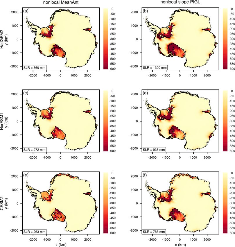
W. H. Lipscomb et al.: CISM Antarctic projections                                                                               635

2     Model and experimental description                            tion for the mean horizontal velocity, followed by a verti-
                                                                    cal integration at each vertex to obtain the full 3D velocity.
2.1    The Community Ice Sheet Model                                This solver gives a good balance between accuracy and ef-
                                                                    ficiency in idealized settings and over the whole ice sheet
CISM is a parallel, higher-order ice sheet model designed           (Leguy et al., 2020; Lipscomb et al., 2019). In Sect. 4.2.2, we
to perform both idealized and whole-ice-sheet simulations           compare DIVA to the more expensive BP solver in selected
on timescales of decades to millennia. It is a descendant           runs.
of the Glimmer model (Rutt et al., 2009) and is now an                 CISM supports several basal friction laws. Most simula-
open-source code developed mainly at the National Center            tions in this study use a power law:
for Atmospheric Research, where it serves as the dynamic
                                                                                   1
ice sheet component of the Community Earth System Model             τ b ≈ Cp |ub | m −1 ub ,                                    (1)
(CESM, http://www.cesm.ucar.edu/models/cesm2/, last ac-
cess: 25 January 2021). The most recent documented re-              where τ b is the basal shear stress, ub is the basal ice ve-
lease was CISM v2.1 (Lipscomb et al., 2019), coinciding             locity, m = 3 is a power-law exponent, and Cp is an em-
with the 2018 release of CESM2 (Danabasoglu et al., 2020).          pirical coefficient for power-law behavior. For a subset of
The model performs well for community benchmark exper-              simulations (Sect. 4.2.4), we use a friction law based on
iments, including the ISMIP-HOM experiments for higher-             Schoof (2005), with a functional form suggested by Asay-
order models (Pattyn et al., 2008) and several stages of            Davis et al. (2016):
the Marine Ice Sheet Model Intercomparison Project: the
                                                                                    Cp Cc N                  1
original MISMIP (Pattyn et al., 2012), MISMIP3d (Pattyn             τb = h                                    m −1 ub ,
                                                                                                    i 1 |ub |                   (2)
et al., 2013), and MISMIP+ (Asay-Davis et al., 2016; Corn-                   Cpm |ub | + (Cc N )m
                                                                                                     m

ford et al., 2020). CISM participated in two earlier ISMIP6
projects focused on ice sheet model initialization: initMIP-        where N is the effective pressure and Cc is an empirical coef-
Greenland (Goelzer et al., 2018) and initMIP-Antarctica             ficient for Coulomb behavior. In the ice sheet interior, where
(Seroussi et al., 2019). More recently, CISM results were           the ice is relatively slow-moving with high effective pressure,
submitted for the ISMIP6 projections (Goelzer et al., 2020;         this law asymptotes to power-law behavior, Eq. (1). Where
Seroussi et al., 2020), the LARMIP-2 experiments (Lever-            the ice is fast-moving with low effective pressure, we have
mann et al., 2019), and the Antarctic BUttressing Model In-         Coulomb behavior:
tercomparison Project (ABUMIP; Sun et al., 2020).
   CISM runs on a structured rectangular grid with a terrain-                     ub
                                                                    τ b ≈ Cc N         .                                        (3)
following vertical coordinate. Most simulations in this paper                    |ub |
were run on a 4 km grid, as for the CISM contributions to           Since the power-law coefficient is spatially variable and
the ISMIP6 Antarctic projections (Seroussi et al., 2020). At        poorly constrained, we use it as a tuning factor, adjusting
4 km resolution, grounding lines are under-resolved, but this       Cp (x, y) for grounded ice to minimize the difference be-
is the finest resolution that permits a large suite of whole-       tween the simulated and observed ice thickness. This tuning
Antarctic simulations at reasonable computational cost. To          is described in Sect. 3.1. Following Asay-Davis et al. (2016),
test sensitivity to grid resolution, we repeated some experi-       the dimensionless Coulomb coefficient is set to Cc = 0.5. As
ments on 8 and 2 km grids (Sect. 4.2.1). All simulations were       in Leguy et al. (2014), the effective pressure is given by
run with five vertical levels. Increasing the number of ver-
tical levels would not substantially change the results, es-                              Hf p

pecially in regions dominated by basal sliding rather than          N (p) = ρi gH 1 −           ,                              (4)
                                                                                          H
vertical shear (i.e., the regions critical for grounding-line re-
treat and SLR). Scalars (e.g., ice thickness H and tempera-         where ρi is ice density, g is gravitational acceleration, Hf =
ture T ) are located at grid cell centers, with horizontal ve-      max(0, − ρρwi b) is the flotation thickness, ρw is seawater den-
locity u = (u, v) computed at vertices. The dynamical core          sity, and b is the bed elevation, defined as negative below
has parallel solvers for a hierarchy of approximations of the       sea level. The parameter p represents the hydrological con-
Stokes stress-balance equations, including the shallow-shelf        nectivity of the subglacial drainage system to the ocean and
approximation (MacAyeal, 1989), a depth-integrated higher-          varies between zero (no connectivity, with N equal to over-
order approximation (Goldberg, 2011), and the 3D Blatter–           burden pressure) and 1 (strong connectivity, with N ap-
Pattyn (BP) higher-order approximation (Blatter, 1995; Pat-         proaching zero near the grounding line).
tyn, 2003). The latter two approximations are classified               CISM also supports several calving laws, but none were
as L1L2 and LMLa, respectively, in the terminology of               found to give calving fronts in good agreement with obser-
Hindmarsh (2004). The simulations for this paper use the            vations for both large and small Antarctic ice shelves. In-
depth-integrated solver, known as DIVA (depth-integrated-           stead, we use a no-advance calving mask, removing all ice
viscosity approximation), which solves a 2D elliptic equa-          that flows beyond the observed calving front. The calving

https://doi.org/10.5194/tc-15-633-2021                                                         The Cryosphere, 15, 633–661, 2021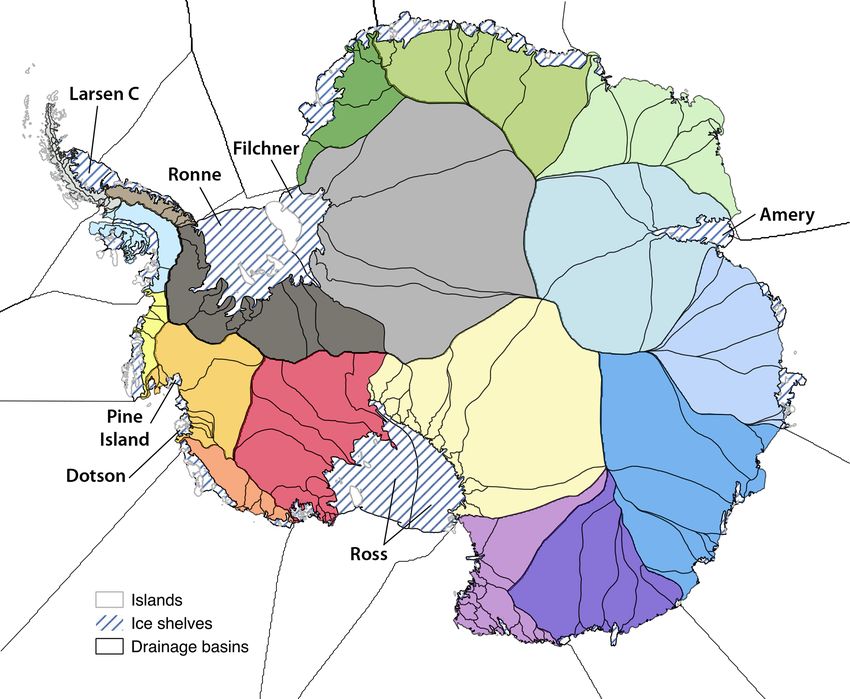
636                                                                      W. H. Lipscomb et al.: CISM Antarctic projections

front can retreat where there is more surface and basal melt-      versity in climate evolution. For CMIP6 models, there was
ing than advective inflow, but more often the calving front        not time for a formal selection, but output from selected mod-
remains in its initial position. For a subset of experiments       els was processed as it became available. Each experiment
(Sect. 4.2.3), we apply additional masks to force the collapse     runs for 86 years, from the start of 2015 to the end of 2100.
of selected ice shelves.                                           Model initialization methods are left to the discretion of each
   Many studies (e.g., Pattyn, 2006; Schoof, 2007) have em-        group and are detailed for specific models in Seroussi et al.
phasized the challenges of simulating ice dynamics in the          (2019, 2020). If the initialization date is before the start of
transition zone between grounded and floating ice, especially      the projections, a short historical run is needed to advance
when the grid resolution is ∼ 1 km or coarser, as is the case      the ISM to the end of 2014.
for most simulations of whole ice sheets. Grounding-line               For projections, ISMIP6 provides data sets of annual-mean
parameterizations (GLPs), which give a smooth transition           atmosphere and ocean forcing on standard grids. The ocean
in basal shear stress across the transition zone, have been        forcing consists of 3D fields of thermal forcing (i.e., the dif-
shown to improve numerical accuracy in models with rela-           ference between the in situ ocean temperature and the in situ
tively coarse grids (e.g., Gladstone et al., 2010; Leguy et al.,   freezing temperature), as described by Jourdain et al. (2020).
2014; Seroussi et al., 2014). Our experiments use a GLP de-        It is not possible to use ocean temperature and salinity di-
scribed by Leguy et al. (2020). For staggered grid cells (i.e.,    rectly from ESMs, because current CMIP models do not sim-
cells centered on the velocity u) that contain the grounding       ulate ocean properties in ice shelf cavities. Moreover, global
line, the basal friction is weighted by the area fraction φg of    ocean models are usually run at a resolution of ∼ 1◦ , too
grounded ice, as determined from a flotation function defined      coarse to give an accurate mean ocean state near Antarctic
at adjacent cell centers:                                          ice shelves. Instead, Jourdain et al. (2020) combined recent
                                                                   data sets (Locarnini et al., 2019; Zweng et al., 2019; Good
ffloat = −b − (ρi /ρw )H.                                   (5)    et al., 2013; Treasure et al., 2017), spanning the years 1995–
Values of ffloat are negative, positive, and zero, respectively,   2018, to construct a 3D gridded climatology of ocean tem-
for grounded ice, floating ice, and along the grounding line.      perature and salinity. This climatology was interpolated to
In Sect. 4.2.1, we test the sensitivity of results to changes in   fill gaps and extrapolated into ice-shelf cavities. To obtain
grid resolution.                                                   forcing fields for projections, temperature and salinity from
   Finally, CISM supports several parameterizations of sub-        the various ESM ocean models were extrapolated to cavi-
ice-shelf melting. For Antarctic projections, the melt param-      ties, and their anomalies were added to the observationally
eterizations are based on ISMIP6 protocols (Sect. 2.2). As         derived climatology. The result is a time-varying 3D product
with basal friction, CISM uses a GLP for basal melting; melt       that can be vertically interpolated to give the thermal forcing
in grid cells containing the grounding line is weighted by the     at the base of a dynamic ice shelf at any time and location in
floating area fraction, 1 − φg . Some studies (e.g., Seroussi      the Antarctic domain. The extrapolation procedure does not
and Morlighem, 2018) have argued that melt should not be           directly resolve ocean circulation in cavities but was seen as a
allowed in partly grounded cells. For CISM, however, Leguy         necessary simplification in the absence of output from high-
et al. (2020) found that applying some melt in these cells         resolution regional ocean models.
improves numerical convergence as a function of resolution,            To compute basal melt rates beneath ice shelves, ISMIP6
at least for idealized configurations with strong buttressing      models can use a standard approach, an open approach, or
(Asay-Davis et al., 2016).                                         both. The open approach is chosen independently by each
                                                                   modeling group; the only requirement is to use the ocean
2.2   Protocols based on ISMIP6 for Antarctic                      data provided by Jourdain et al. (2020). For the standard ap-
      projections                                                  proach, basal melt rates beneath ice shelves are computed as
                                                                   a quadratic function of thermal forcing as described by Favier
Protocols for the ISMIP6 Antarctic projections are described       et al. (2019), with a thermal forcing correction suggested by
in detail by Nowicki et al. (2020) and Jourdain et al. (2020).     Jourdain et al. (2020):
Here, we give a brief summary, noting where the simula-                                         2
tions in this study differ from the protocols. The ISMIP6                               ρw cpw
                                                                   m(x, y) = γ0 ×                     × (TF(x, y, zdraft ) + δTsector )
projection experiments are run with standalone ISMs, forced                             ρi Lf
by time-varying, annual-mean atmosphere and ocean fields             × |hTFidraft∈sector + δTsector | ,                                   (6)
derived from the output of CMIP5 and CMIP6 ESMs. In
our study, the projection experiments use ocean forcing that       where m is the melt rate, TF is the thermal forcing, γ0 is an
evolves during the simulation, but the atmospheric forcing         empirical coefficient, ρw and cpw are the density and specific
(specifically, the SMB) is held to the values used when spin-      heat of seawater, and ρi and Lf are the density and latent
ning up the model. The CMIP5 models were selected by               heat of melting of ice. The brackets in < TF > denote the
a procedure described by Barthel et al. (2020) to represent        average over a drainage basin or sector, and δTsector is a ther-
present-day Antarctic conditions well and to sample the di-        mal forcing correction with units of temperature, with one

The Cryosphere, 15, 633–661, 2021                                                          https://doi.org/10.5194/tc-15-633-2021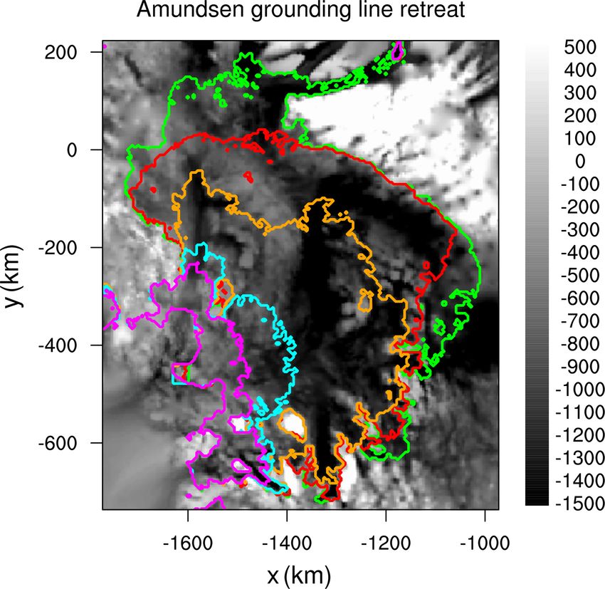
W. H. Lipscomb et al.: CISM Antarctic projections                                                                                   637

value per sector. The Antarctic Ice Sheet is divided into 16          Table 1. Calibrated γ0 values for the three quadratic parameteriza-
sectors as shown in Fig. 1. Since this method uses sector-            tions and two calibration methods (in m yr−1 ).
average thermal forcing, it is known as the nonlocal param-
eterization. For the simulations in this paper, the last term                   Parameterization    Calibration        γ0
in Eq. (6) is modified to max(hTFidraft∈sector + δTsector , 0),                 Local               MeanAnt        1.11 × 10⁴
to prevent spurious melting and freezing in sectors where                       Nonlocal            MeanAnt        1.44 × 10⁴
hTFidraft∈sector + δTsector < 0. The nonlocal quadratic depen-                  Nonlocal-slope      MeanAnt        2.06 × 10⁶
dence on TF in Eq. (6) is based on the idea that the melt rate                  Local               PIGL           4.95 × 10⁴
is proportional to the local TF and also to the speed of the                    Nonlocal            PIGL           1.59 × 10⁵
sub-shelf flow, which in turn is proportional to the regional                   Nonlocal-slope      PIGL           5.37 × 10⁶
mean TF.
   An alternative local parameterization is obtained by re-
placing hTFidraft∈sector with TF (x, y, zdraft ) in the last term:
                                                                      of grounded and floating ice near the grounding line, as de-
                    ρw cpw 2

                                                                      scribed in Sect. 3.1. This procedure is motivated by the fact
m(x, y) = γ0 ×
                    ρi Lf                                             that ice thickness is better constrained than melt rates, and
                                         2                         future projections are sensitive to the initial grounding-line
   × max TF(x, y, zdraft ) + δTsector , 0 ,                     (7)   position (Seroussi et al., 2019). Thus, δTsector is calibrated to
giving a quadratic dependence on the local thermal forcing.           obtain melt rates that will drive the ice toward the observed
A third parameterization, which we call nonlocal-slope, is            extent and thickness, but the basin-average melt rates will
obtained by multiplying Eq. (6) by sin(θ ), where θ is the lo-        differ from observational estimates.
cal angle between the ice-shelf base and the horizontal. At              In summary, we have presented three basal melt param-
the same time, γ0 is increased by a factor of ∼ 100, since            eterizations (local, nonlocal, and nonlocal-slope) and two
sin(θ ) typically is ∼ 10−2 near grounding lines. This scheme,        calibration methods (MeanAnt and PIGL), giving six possi-
suggested by Little et al. (2009) and Jenkins et al. (2018),          ble combinations (local-MeanAnt, nonlocal-PIGL, etc.). The
generally gives larger melt rates near grounding lines and            values of γ0 for each combination, shown in Table 1, corre-
lower melt rates near calving fronts, in agreement with obser-        spond to the median values in Jourdain et al. (2020). These
vational estimates and ocean simulations (e.g., Rignot et al.,        combinations form the basis for the spin-up and forcing ex-
2013; Favier et al., 2019). Total melt over the ice sheet is          periments described in Sects. 3 and 4.
the same, if γ0 is tuned based on a total-melt criterion as in
Jourdain et al. (2020). CISM simulations in Seroussi et al.
(2020) used this nonlocal-slope parameterization as an open           3     Model spin-up
approach.
   Sub-ice-shelf thermal forcing and melt rates are uncertain,        3.1    Spin-up procedure
as is the functional relationship between thermal forcing and
melt rates. For this reason, γ0 and δTsector are not well con-        When spinning up the model, we aim to reach a stable state
strained and can be viewed as tuning parameters. To calibrate         with minimal drift under modern forcing, while also simu-
Eqs. (6) and (7), Jourdain et al. (2020) used two methods. In         lating ice sheet properties that agree with observations. It is
the MeanAnt method, γ0 is chosen so that the total Antarctic          challenging to achieve both goals at once. Long spin-ups typ-
melt rate given by the parameterization matches the observa-          ically yield a steady-state ice sheet with large biases in thick-
tional estimates of Depoorter et al. (2013) and Rignot et al.         ness, velocity, and/or ice extent, while initialization methods
(2013), before applying basin-scale thermal forcing correc-           that assimilate data to match present-day conditions often
tions. Then the δTsector values are chosen to reproduce the           have a large initial transient. We compromised by using a hy-
estimated mean melt rate in each sector. The PIGL method              brid method similar to that of Pollard and DeConto (2012),
is similar, except that the melt-rate targets are given by ob-        running a long spin-up while continually nudging the ice
servations in the Amundsen sector near the grounding line of          sheet toward the observed thickness.
Pine Island Glacier (Rignot et al., 2013). The γ0 values for             Beneath grounded ice, we adjust Cp (x, y), a poorly con-
the PIGL calibration are an order of magnitude larger than            strained, spatially varying coefficient in the basal friction law,
those obtained by the MeanAnt method, but the present-day             Eqs. (1) or (2). This coefficient controls the power-law be-
average melt rates in each basin are similar with the two cal-        havior, with higher Cp giving more friction and slower slid-
ibrations. See Jourdain et al. (2020) for more details on these       ing. Wherever grounded ice is present, Cp is initialized to
parameterizations and calibrations.                                   20 000 Pa m(−1/3) yr(1/3) . During the spin-up, Cp is decreased
   The simulations in our paper differ from the ISMIP6 proto-         where H > Hobs and increased where H < Hobs , based on
cols in the treatment of δTsector . Although we use calibrated        the idea that lower friction will accelerate the ice and lower
values of γ0 , we tune δTsector to better match the thickness         the surface, while higher friction will slow the ice and raise

https://doi.org/10.5194/tc-15-633-2021                                                         The Cryosphere, 15, 633–661, 2021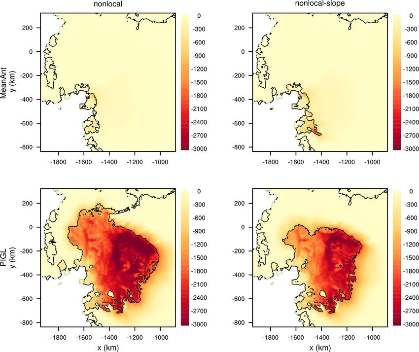
638                                                                            W. H. Lipscomb et al.: CISM Antarctic projections

Figure 1. Antarctic sectors (colors) defined by Mouginot et al. (2017) and Rignot et al. (2019). Eighteen sectors are shown, but 16 sectors
are used in this study, with sectors combined in the Ross and Filchner–Ronne basins. Reprinted with permission from Jourdain et al. (2020,
their Fig. 2).

the surface. The rate of change of Cp is given by                          A different method is needed to initialize floating ice
                                                                      shelves, where Cp = 0. In CISM simulations for initMIP-
dCp        Cp (H − Hobs )       dH
      =−                     +2       ,                        (8)      Antarctica (Seroussi et al., 2019) and the ISMIP6 projec-
  dt      H0         τc          dt                                     tions (Seroussi et al., 2020), basal melt rates were obtained
where Hobs is an observational target, H0 = 100 m is a thick-           by local nudging. That is, an equation similar to Eq. (8) was
ness scale, and τc = 500 years is a timescale for adjusting Cp .        used to nudge H toward Hobs by adjusting the melt rate
The first term in brackets nudges H toward Hobs , and the sec-          m(x, y) in each floating grid cell. In climate change experi-
ond term damps the nudging to prevent overshoots. We hold               ments, the spun-up melt rates were added to melt-rate anoma-
Cp within a range between 102 and 105 Pa m(−1/3) yr(1/3) .              lies in each basin. This method yields ice-shelf thicknesses
Smaller values can lead to excessive sliding speeds when                and grounding-line locations that agree well with observa-
the basal friction approaches zero. With Cp at its maximum              tions, but it overfits the observations, giving noisy melt rates
value, basal sliding is close to zero, and there is little benefit      that compensate for other errors without being tied to ocean
in raising Cp further.                                                  temperatures. Other complications arise when applying this
   This method works well at keeping most of the grounded               spin-up method to the ISMIP6 projections, which prescribe
ice near the observed thickness. Also, since Cp is indepen-             thermal forcing anomalies instead of melt-rate anomalies. In
dent of the ice thermal state, we remove low-frequency oscil-           climate change experiments, a melt-rate anomaly computed
lations associated with slow changes in basal temperature, re-          from the thermal forcing anomaly must be added to the spun-
sulting in a better-defined steady state. In forward runs, how-         up melt rate, instead of computing the evolving melt rate di-
ever, Cp (x, y) is held fixed and cannot evolve in response to          rectly from the evolving thermal forcing.
changes in basal temperature or hydrology. As a result, we                 For the simulations described here (which were done too
can have unphysical basal velocities when the ice dynamics              late to be included in Seroussi et al., 2020), we take a dif-
differs from the spun-up state. Also, the tuning of Cp can              ferent approach. During the spin-up, basal melt rates are
compensate for other errors. For example, if the prescribed             computed directly from the thermal forcing, using the cli-
topography is missing pinning points near the grounding line,           matological data set and melt parameterizations described
the ice will be biased thin, and Cp can be driven to high val-          in Sect. 2.2. When we use the calibrated values of both γ0
ues to make up for the lack of buttressing.

The Cryosphere, 15, 633–661, 2021                                                             https://doi.org/10.5194/tc-15-633-2021
W. H. Lipscomb et al.: CISM Antarctic projections                                                                               639

and δTsector , many grounding lines drift far from their ob-        where glaciers are losing mass. We compensated for disequi-
served locations. The drift can be reduced (but not elimi-          librium by increasing the target thickness for this sector by
nated) by continually adjusting δTsector in each of 16 sectors      the equivalent of 1000 Gt of ice, roughly the mass lost by
(see Fig. 1), nudging toward an ice thickness target in a re-       Pine Island Glacier in recent decades (Rignot et al., 2019).
gion near the grounding line. Here, “near the grounding line”       With this adjustment, the advance of the Pine Island ground-
is defined as having ffloat (see Eq. 5) with a magnitude less       ing line from the present location to a more stable position
than a prescribed value:                                            downstream (which takes place in all spin-ups) does not have
                                                                    to be compensated by retreat elsewhere in the sector. Other-
                   ρi                                               wise, we assumed that the recent mass loss is small enough
|ffloat | = −b −      H < Hthresh ,                          (9)
                   ρw                                               that the present-day ice thickness is an appropriate target.
                                                                       The spin-ups are run for 20 000 model years, allowing the
where Hthresh is a prescribed threshold thickness. We set           ice sheet to approach steady state; at this time the total mass
Hthresh = 500 m so that the target region includes most of the      is changing by < 1 Gt yr−1 . We evaluate the spun-up state
ice likely to switch between floating and grounded during a         below.
spin-up, without extending too far upstream.
   During the spin-up, δTsector is adjusted as follows:             3.2   Spun-up model state

d(δTsector )      1          H̄ − H̄obs    dH̄                      To initialize the standard projection experiments described
             =−                         +2     ,            (10)
    dt          τm mT           τm          dt                      in Sect. 4.1, we carried out six Antarctic spin-ups, each
                                                                    with a different pairing of the three basal melt parameteri-
where H̄ is the mean ice thickness over the target re-              zations (local, nonlocal, and nonlocal-slope) and the two cal-
gion, H̄obs is the observational target for this region, mT =       ibrations (MeanAnt and PIGL). Although γ0 varies widely
10 m yr−1 ◦ C−1 is a scale for the rate of change of basal melt     among the different spin-ups (Table 1), the spun-up states are
rate with temperature, and τm = 100 yr is a timescale for ad-       similar across parameterizations and calibrations, because of
justing δT . As in Eq. (8), the first-derivative term damps         the freedom to adjust Cp and δTsector independently for each
oscillations. In most basins, this adjustment keeps H̄ close        run to match the observed thickness. The simulated thick-
to H̄obs with |δTsector | < 1 ◦ C. In basins where H̄ < H̄obs no    ness, velocity, and ice extent are broadly in agreement with
matter how much δTsector is lowered, δTsector is capped at          observations, but with some persistent biases. Some biases
−2 ◦ C.                                                             can be attributed to errors in ocean thermal forcing (which
   Given the calibrated thermal forcing, the melt rate m is         is treated simply by the basin-scale melt parameterizations)
computed for floating grid cells using one of the three param-      and seafloor topography (e.g., an absence of pinning points,
eterizations described in Sect. 2.2. In partly grounded cells,      resulting in grounding-line retreat that is compensated for
m is weighted by the floating ice fraction. In shallow cavi-        by spurious ocean cooling). Pinning points could either be
ties, following Asay-Davis et al. (2016), m is weighted by          missing in the high-resolution (0.5 km) topographic data set
tanh(Hc /Hc0 ), where Hc is the cavity thickness and Hc0 =          (Morlighem et al., 2019) or smoothed away when interpolat-
50 m is an empirical depth scale.                                   ing to the coarser CISM grid.
   For each spin-up, the ice sheet is initialized to the present-      Figure 2 shows the difference between the final ice thick-
day thickness using the BedMachineAntarctica data set               ness and the observed thickness for two spin-ups: nonlocal-
(Morlighem et al., 2019). The internal ice temperature is           MeanAnt and nonlocal-slope-PIGL. Figure 3 is like Fig. 2,
initially set to an analytic vertical profile and then evolves      but focused on the Amundsen sector. These two melt
freely under advection. The surface mass balance and sur-           schemes are interesting to compare because, as shown in
face temperature are provided by a regional climate model,          Sect. 4.1, the latter is much more sensitive to ocean warming.
RACMO2.3 (van Wessem et al., 2018), and the geothermal              The spun-up states, however, are similar, with some shared
heat flux is from Shapiro and Ritzwoller (2004). As described       biases. In both spin-ups, Thwaites Glacier is too thin near
above, Cp is adjusted in grounded cells to better match the         the grounding line, while Pine Island Glacier is too thick, as
observed local ice thickness, and δTsector is adjusted in each      are the Crosson and Dotson ice shelves. The Filchner–Ronne
of the 16 sectors to match the observed thickness of ice near       Ice Shelf is thin near the central grounding line but thick else-
the grounding line.                                                 where, and there are similar thick–thin patterns for the Ross
   Since the spun-up ice sheet represents a quasi-equilibrium       Ice Shelf. There are also a few differences; for example, the
state before the mass loss of the past few decades, we as-          George VI Ice Shelf and the seaward parts of the Amery and
signed a date of 1950 to the spin-up. In sectors where the          Larsen C shelves are thinner in the nonlocal-MeanAnt run.
thermal forcing in the climatology exceeds the forcing that            Figure 4 compares ice surface speeds from the end of the
was typical in the mid-20th century and before, δTsector can        nonlocal-MeanAnt spin-up to observed surface speeds (Rig-
compensate by becoming more negative. The ice sheet is              not et al., 2011). Overall, the agreement with observations is
out of equilibrium today, especially in the Amundsen sector         very good for both grounded and floating ice, even though the

https://doi.org/10.5194/tc-15-633-2021                                                       The Cryosphere, 15, 633–661, 2021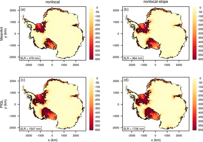
640                                                                              W. H. Lipscomb et al.: CISM Antarctic projections

Figure 2. Change in ice thickness (m) between the start and end of two 20 kyr CISM spin-ups at 4 km resolution, for two combinations of melt
parameterization and calibration: (a) nonlocal-MeanAnt and (b) nonlocal-slope-PIGL. The initial state is based on observations (Morlighem
et al., 2019), and positive values indicate where the spun-up ice state is thicker than observed. Black lines show boundaries of floating ice at
the end of each spin-up.

Figure 3. Same as Fig. 2, but focused on the Amundsen sector.

model is nudged toward observed velocities only indirectly,                  For the same spin-up, Fig. 5 shows ice surface speeds in
via the thickness field. In general, good agreement in thick-             the Amundsen sector, including Pine Island and Thwaites
ness implies agreement in velocity as well, at least when us-             glaciers. The observations reveal a dual structure in the
ing BedMachineAntarctica thicknesses, which are obtained                  Thwaites velocity field, with a fast western core where the
using the mass conservation method of Morlighem et al.                    glacier flows into the Thwaites Ice Tongue and slower speeds
(2011). One place of disagreement is the Kamb Ice Stream                  in the east where flow is impeded by an ice rise (see Fig. 1
(on the Siple Coast of the Ross Ice Shelf), which is clearly              in Rignot et al., 2014). The model, however, lacks a sharp
visible in the model but absent in the observations, having               division between east and west, and the Thwaites grounding
stagnated in the 1800s and left a signature in the thickness              line is retreated compared to observations, perhaps because
field (Ng and Conway, 2004).                                              interaction with seafloor topography is not captured accu-
                                                                          rately. At the same time, the Pine Island grounding line is

The Cryosphere, 15, 633–661, 2021                                                                https://doi.org/10.5194/tc-15-633-2021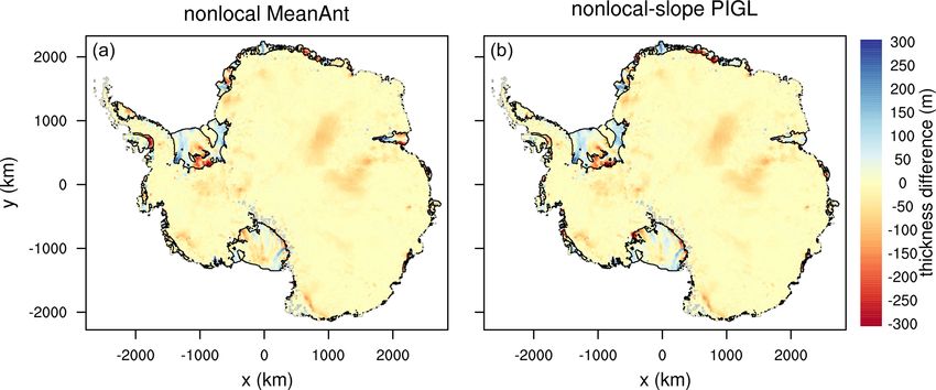
W. H. Lipscomb et al.: CISM Antarctic projections                                                                                         641

Figure 4. Antarctic ice surface speed (m yr−1 , log scale) from (a) observations (Rignot et al., 2011) and (b) the end of a 20 kyr CISM spin-up
at 4 km resolution using the nonlocal-MeanAnt melt parameterization and calibration.

Figure 5. Same as Fig. 4, but focused on the Amundsen sector. Light gray lines show boundaries of floating ice.

advanced compared to observations. The grounding lines of                 needed to curtail the grounding-line retreat that occurs under
both glaciers have been retreating since at least the 1990s               climatological thermal forcing. As a result, the spun-up melt
(Rignot et al., 2014), and the spin-up method is not well                 rates in these regions are lower than observed. Total sub-shelf
suited to initializing dynamic grounding lines in their ob-               melting for Antarctica at the end of the spin-up ranges from
served locations.                                                         625 to 744 Gt yr−1 , about half the values estimated by De-
   Figure 6 shows the values of the thermal forcing correc-               poorter et al. (2013) and Rignot et al. (2013). Negative val-
tion δTsector for each sector at the end of the six spin-ups.             ues of δTsector might be compensating for other errors, such
In most sectors, the corrections are modest (< 1 ◦ C in mag-              as biases in the climatology or the failure of the melt scheme
nitude). For the Aurora sector in East Antarctica, however,               to deliver ocean heat to the right places. Another possibility,
δT is strongly negative, ranging from −1.0 to −1.7 ◦ C de-                considered in Sect. 4.2.5, is that for some sectors, the thermal
pending on the melt scheme and calibration. Also, δTsector is             forcing derived from the 1995–2018 climatology exceeds the
consistently negative for the Amundsen sector, with values                forcing that was typical in the mid-20th century and before.
from −0.7 to −1.8 ◦ C. In both sectors, significant cooling is            In this case, δTsector < 0 would be correcting for the recent

https://doi.org/10.5194/tc-15-633-2021                                                              The Cryosphere, 15, 633–661, 2021
642                                                                       W. H. Lipscomb et al.: CISM Antarctic projections

warming, to generate melt rates closer to preindustrial val-        runs, in which the increased melting is concentrated near the
ues.                                                                grounding line, these shelves thin but remain intact.
                                                                       Figure 8 shows the ice thickness change for a uniform
                                                                    TF anomaly of 2 ◦ C. With a doubling of the anomaly, the
4     Results of projection experiments                             SLR contribution more than doubles, reaching nearly 4 m for
                                                                    nonlocal-slope-PIGL. Much of the nonlinearity stems from
After spinning up the model as described in Sect. 3, we ran a       marine ice collapse in the Amundsen sector. For nonlocal-
series of projection experiments. Section 4.1 gives the results     slope-MeanAnt, the Pine Island Glacier basin collapses, and
of what we call the standard experiments, which were run on         for both PIGL runs, the Thwaites basin also collapses, rais-
a 4 km grid using the DIVA solver with a basal friction power       ing sea level by an additional ∼1 m compared to runs without
law, and without prescribing ice-shelf collapse. We ran sev-        Amundsen collapse. For nonlocal-slope-PIGL, the collapse
eral projections with idealized thermal forcing, followed by        creates a continuous ice shelf between the Ross and Amund-
many projections with TF derived from ESMs as in ISMIP6.            sen seas. These runs illustrate a threshold of instability for
Section 4.2 describes the results of sensitivity experiments in     the Amundsen sector, which we discuss further in Sect. 4.2.5.
which the grid resolution, stress-balance approximation, ice-       A threshold in the range 1–2◦ is consistent with the model-
shelf extent, and basal sliding law are varied. We also explore     ing study of Rosier et al. (2020), who found that Pine Is-
the sensitivity of the Amundsen sector to parameter changes.        land Glacier collapses with ocean warming greater than 1.2◦
                                                                    (using a local melt parameterization similar to Eq. 7). A
4.1    Standard experiments                                         TF anomaly of 2 ◦ C also drives significant ice loss in East
                                                                    Antarctica, including the Wilkes, Aurora, and Amery sectors,
We first show results from experiments with idealized, spa-         for all melt schemes except nonlocal-MeanAnt.
tially uniform thermal forcing anomalies. These experiments            Next, we analyze projection experiments with ocean ther-
help identify the regions that are most vulnerable to a given       mal forcing anomalies derived from six CMIP ESMs. The
ocean warming. In the first set of experiments, the TF              four CMIP5 models are CCSM4, HadGEM2-ES (hereafter
anomaly is ramped up linearly by 1 ◦ C between 1950 and             HadGEM2), MIROC-ESM-CHEM (hereafter MIROC), and
2100 and then is held fixed at 1 ◦ C until 2500. The second set     NorESM1-M (hereafter NorESM1). These were among the
is like the first, except that the TF anomaly is ramped up by       six top-ranking models chosen by Barthel et al. (2020).
2 ◦ C. From Eqs. (6) and (7), the melt rate is a quadratic func-    CCSM4, MIROC, and NorESM1 were used for the ISMIP6
tion of thermal forcing, and therefore the incremental change       Tier 1 experiments, and we added HadGEM2 (a Tier 2 selec-
in melt rate is proportional to the product of the initial TF and   tion) to sample a model with relatively high ocean warming.
the TF anomaly. Thus, ice retreat is favored where TF and/or        The two CMIP6 models are CESM2 and UKESM, which
its anomaly are large. The ice sheet response is also sensi-        are successors of CCSM4 and HadGEM2, respectively. All
tive to the bed topography and basal friction, among other          the ESMs ran high-end emissions scenarios: RCP8.5 for the
factors.                                                            CMIP5 models and SSP5-85 for the CMIP6 models. Each
   Figure 7 shows the difference in ice thickness between           spun-up ice sheet state is run forward with ocean forcing
2500 and 1950 for a TF anomaly of 1 ◦ C, using the non-             from each of the six ESMs.
local and nonlocal-slope melt parameterizations with the               As described in Sect. 2.2, the thermal forcing is derived by
MeanAnt and PIGL calibrations. Results with the local melt          adding ESM temperature and salinity anomalies to a back-
scheme (not shown) are similar to those with the nonlocal           ground climatology and then extrapolating into sub-shelf
scheme. All four experiments show significant thinning of           cavities. Figure 9 shows the thermal forcing at ocean level
the four largest ice shelves (Ross, Filchner–Ronne, Amery,          9 (z = −510 m) for each ESM, averaged over 2081–2100.
and Larsen C) as well as small shelves (e.g., in the Amund-         For each model, the forcing is relatively uniform across a
sen sector and East Antarctica). Thinning of grounded ice           given basin. The Amundsen sector is the warmest of the
is concentrated in the Filchner–Ronne and Ross sectors of           three large WAIS basins, as a result of warm CDW penetrat-
West Antarctica and is modest for the Amundsen sector.              ing into sub-shelf cavities (Holland et al., 2020). HadGEM2
The loss of ice mass above flotation, which contributes di-         and UKESM are both relatively warm in the Filchner–Ronne
rectly to SLR, ranges from 479 mm sea-level equivalent              basin and less warm in the Ross basin. NorESM1 is mod-
(s.l.e.) for nonlocal-MeanAnt to 1726 mm s.l.e. for nonlocal-       erately warm for Filchner–Ronne and especially warm for
slope-PIGL. For the Ross and western Ronne sectors, the             Ross. CCSM4 and (to a lesser extent) CESM2 are moder-
PIGL runs have much more grounding-line retreat and mass            ately warm for Filchner–Ronne, but both are fairly cold for
loss than do the MeanAnt runs. The nonlocal runs, unlike            Ross, while MIROC is moderately warm for Ross and cold
the nonlocal-slope runs, have substantial basal melting far         for Filchner–Ronne. These patterns are reflected in the ice
from the grounding line, leading to calving-front retreat.          loss discussed below.
For nonlocal-PIGL, the four largest shelves disappear by               Figure 10 shows the TF anomaly at z = −510 m for
2500 with the increased basal melting. For the nonlocal-slope       each ESM, averaged over 2081–2100 and with respect to

The Cryosphere, 15, 633–661, 2021                                                       https://doi.org/10.5194/tc-15-633-2021
W. H. Lipscomb et al.: CISM Antarctic projections 643 Figure 6. Values of the thermal forcing correction δTsector (◦ C) in each of 16 Antarctic sectors for six combinations of melt parameterization (local, nonlocal, and nonlocal-slope) and calibration (MeanAnt and PIGL). (a) ISMIP6 values, calibrated based on sub-shelf melt rates. Values for the local and nonlocal parameterizations were reported by Jourdain et al. (2020); values for nonlocal-slope were computed for this study. (b) Values obtained during CISM spin-ups. Figure 7. Difference in ice thickness (m) between the years 2500 and 1950 in experiments with idealized ocean forcing. Starting from the spun-up state, thermal forcing increases by 1 ◦ C between 1950 and 2100 and is held fixed thereafter. The two columns correspond to the nonlocal and nonlocal-slope melt parameterizations, and the two rows to the MeanAnt and PIGL calibrations. Black lines show boundaries of floating ice at the end of each run. In the nonlocal-PIGL run (c), black lines at the present-day calving fronts of several large ice shelves are absent, indicating shelf collapse. In the nonlocal-MeanAnt run (a), the Ross Ice Shelf partly collapses. Boxes in the lower left of each panel show the SLR contribution from the loss of grounded ice. https://doi.org/10.5194/tc-15-633-2021 The Cryosphere, 15, 633–661, 2021
644                                                                            W. H. Lipscomb et al.: CISM Antarctic projections

Figure 8. Same as Fig. 7, but with thermal forcing increasing by 2 ◦ C between 1950 and 2100 and held fixed thereafter. In the nonlocal runs
(a, c), black lines are absent at the present-day calving fronts of several ice shelves, indicating shelf collapse.

Figure 9. Ocean thermal forcing (◦ C) at z = −510 m, averaged over 2081–2100, for the four CMIP5 models and two CMIP6 models used
in ocean-forced projection experiments. Thermal forcing is used to compute basal melt rates in grid cells with floating ice.

The Cryosphere, 15, 633–661, 2021                                                              https://doi.org/10.5194/tc-15-633-2021
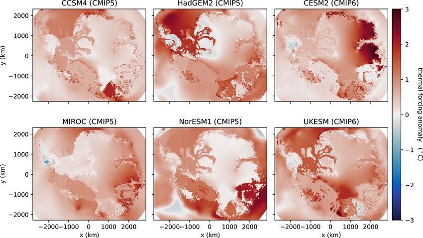
W. H. Lipscomb et al.: CISM Antarctic projections                                                                             645

the 1941–1960 average. For the Filchner–Ronne basin, the           more SLR than local and nonlocal, and the PIGL calibra-
anomalies are largest (∼ 2 ◦ C) for HadGEM2 and UKESM,             tion gives more SLR than MeanAnt. The greater sensitivity
while NorESM1 has the largest anomalies for the Ross basin.        for the nonlocal-slope runs can be attributed to larger melt
The anomalies are ∼1 ◦ C or less for the Amundsen sector.          rates at steep slopes near grounding lines, where melting is
Thus, most of the Amundsen thermal forcing in Fig. 9 is al-        most effective in driving ice retreat. The greater sensitivity
ready present in the contemporary (1995–2018) background           of PIGL compared to MeanAnt follows from the larger γ0 .
climatology, to which ESM anomalies are added. To the ex-          During the spin-ups, PIGL runs acquire more negative values
tent that the Amundsen sector has warmed in recent decades,        of δTsector than MeanAnt (Fig. 6), to compensate for greater
the ESMs appear not to fully capture the warming, perhaps          γ0 . Then, for a given TF anomaly during the forward runs,
because they are too coarse to simulate CDW-driven warm-           the increase in m is proportional to γ0 and thus is larger for
ing. Also, an ESM might already have a warm Amundsen               PIGL.
sector (with CDW having access to the sub-shelf cavity) in            Third, the CMIP model rankings are consistent across
its mid-20th-century climate, with the result that subsequent      melt schemes. HadGEM2 and UKESM are the warmest
warming is small.                                                  models and drive the most SLR, followed in most cases
   Each projection experiment is run for 550 years starting        by NorESM1. CCSM4 and CESM2 are next, and MIROC
at the end of 1950, the nominal date of the spin-up. In the        yields the least SLR. This ranking reflects the magnitude of
ISMIP6 protocols, the first 64 years (to the start of 2015)        the thermal forcing and its anomaly in the various WAIS
constitute a historical run and the remainder a projection run,    basins (Figs. 9 and 10). For a given ESM, the most sensi-
but for our simulations the historical and projection periods      tive melt scheme (nonlocal-slope-PIGL) yields 3 to 4 times
are forced in the same way. From 1951–2100, we apply the           as much SLR as the least sensitive schemes (local- and
annual-mean thermal forcing provided by ISMIP6, consist-           nonlocal-MeanAnt), and the warmest models (HadGEM2
ing of ESM anomalies added to the background climatology.          and UKESM) drive 2 to 3 times as much SLR as the coolest
After 2100, we cycle repeatedly through the last 20 years          (MIROC). Thus, the total SLR over 550 years varies by an
of forcing, 2081–2100, to evaluate the committed SLR asso-         order of magnitude, from ∼ 150 to 1300 mm.
ciated with a late-21st-century climate. For comparison, we           Figure 12 shows spatial plots of thickness changes from
ran a subset of forcing experiments using a fixed climatol-        projection runs with forcing from three ESMs (HadGEM2,
ogy, computed as the mean of the 2081–2100 thermal forc-           NorESM1, and CESM2) with nonlocal-MeanAnt and
ing. Cycling through the annual forcing drives greater mass        nonlocal-slope-PIGL, the least and most sensitive melt com-
loss (by ∼ 15 %) than does the fixed climatology, suggesting       binations. Ice loss for HadGEM2 is similar to that for a
that years with high thermal forcing have a disproportionate       uniform TF anomaly of 1 ◦ C (Fig. 7), and NorESM1 and
influence on long-term mass loss, because of the quadratic         CESM2 have somewhat smaller losses. As in the experi-
relationship between thermal forcing and melt rates.               ments with a uniform TF anomaly, most of the SLR con-
   Figure 11 shows time series of ocean-forced SLR                 tribution comes from the Filchner–Ronne and Ross sectors,
for 36 projection experiments, with one panel per                  with only a small Amundsen contribution. Compared to the
parameterization–calibration pair. Along with the ESM-             WAIS, the SLR contribution from East Antarctica is small,
forced runs, each plot shows the SLR from a control run with       apart from the Amery sector in the nonlocal-slope-PIGL
no change in thermal forcing compared to the spin-up. In           runs. As seen in Figs. 7 and 8, the nonlocal-slope scheme
this figure (and in figures below, unless otherwise specified),    drives substantial grounding-line retreat without calving-
results from control runs are not subtracted from projection       front retreat, while the nonlocal scheme can trigger Ross Ice
runs. SLR during the control runs is minimal, confirming that      Shelf collapse, with less grounding-line retreat.
the spin-ups are close to steady state.                               It is possible that the melt parameterizations underesti-
   Several patterns emerge. First, SLR starts slowly for all ex-   mate the delivery of heat to Amundsen grounding lines, in
periments and then accelerates near the end of the 21st cen-       part because of the negative δTsector corrections (Sect. 3.2)
tury, suggesting that a threshold has been crossed based on        and the modest TF anomalies in the ESMs (Fig. 10). Con-
some magnitude or duration of thermal forcing. After 2100,         versely, the extrapolation procedure and melt parameteriza-
SLR is fairly linear and shows no sign of leveling off after       tions might overestimate heat delivery to the Filchner–Ronne
500 years. This is consistent with retreat driven by MISI in       and Ross cavities, which currently have little basal melting.
large reverse-sloping basins. Once the retreat is under way, it    Although some ocean models with CMIP3 atmospheric forc-
continues until reaching a stable seafloor configuration, up to    ing have projected Weddell Sea warming (e.g., Hellmer et al.,
several hundreds of kilometers upstream.                           2012; Timmermann and Hellmer, 2013), it is not clear that
   Second, the ice sheet is more sensitive to some melt com-       these large shelves will readily transition from cold, low-melt
binations than others. The results from local and nonlocal         regimes to warm, high-melt regimes (Naughten et al., 2018).
parameterizations are similar for the MeanAnt runs, but the
nonlocal scheme gives greater SLR (by ∼ 100–200 mm) for
the PIGL runs. The nonlocal-slope parameterization yields

https://doi.org/10.5194/tc-15-633-2021                                                     The Cryosphere, 15, 633–661, 2021
646 W. H. Lipscomb et al.: CISM Antarctic projections
Figure 10. Ocean thermal forcing anomaly (◦ C) at z = −510 m for the four CMIP5 models and two CMIP6 models used in ocean-forced
projection experiments. The anomaly is averaged over 2081–2100 and is computed with respect to the base period 1941–1960.
4.2 Sensitivity experiments more drift during the projection runs. The drift in ice mass at
the end of the 2 km spin-ups is 1 to 5 Gt yr−1 (toward greater
In this section we explore the sensitivity of projected ice loss mass and lower sea level), compared to drift of < 1 Gt yr−1
to changes in model settings and forcing. We vary the grid at the end of the 20 kyr standard spin-ups.
resolution between 2 and 8 km, we replace the DIVA solver The spun-up ice states at 2 and 8 km (not shown) are sim-
with the Blatter–Pattyn solver, we prescribe the collapse of ilar to the 4 km spin-ups (Sect. 3.2). For the projection ex-
selected ice shelves, and we replace the basal friction power periments, the 8 km runs lose less mass than the 4 km runs
law with the Schoof friction law, Eq. (2). We also study the (except for nonlocal-MeanAnt, which has slightly greater ice
sensitivity of the Amundsen sector under different parameter loss), while the 2 km runs lose more mass than the 4 km
choices. runs. Figure 13 shows time series of the difference in cumu-
lative SLR, relative to the respective control runs, between
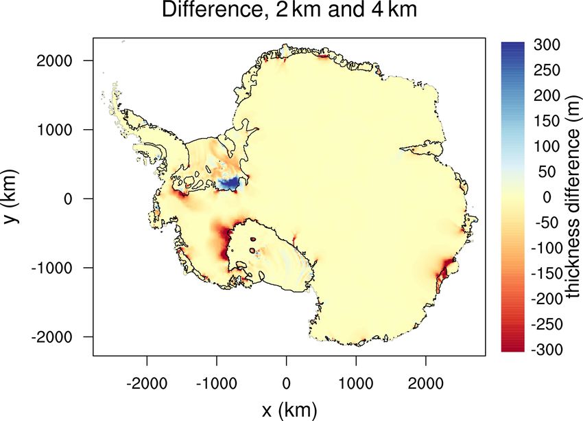
4.2.1 Grid resolution the 8 and 4 km runs (in the left-hand panels) and between
the 2 and 4 km runs (in the right-hand panels). For reference,
Previous studies have found grounding-line retreat to be sen- Fig. 11 shows the 4 km time series. Generally, the SLR dif-
sitive to grid resolution, with finer resolution typically lead- ferences are largest for the runs with the most total ice loss.
ing to greater Antarctic retreat (Cornford et al., 2013, 2015). The 2 km SLR exceeds the 4 km SLR by up to ∼ 15 %, and
In benchmark experiments (Pattyn et al., 2013; Asay-Davis the 4 km SLR exceeds the 8 km SLR by as much as 20 %.
et al., 2016) for marine ice sheets, Leguy et al. (2020) found The largest differences, and the greatest overall ice loss, are
that with GLPs for basal friction and sub-shelf melting, for the nonlocal-slope-PIGL runs forced by HadGEM2, for
CISM results at resolutions of 2 to 4 km are close to the con- which the SLR contributions at 8, 4, and 2 km are 1047 mm,
verged results at 0.5 to 1.0 km. To test CISM’s dependence 1300 mm, and 1473 mm, respectively. Figure 14 shows the
on resolution for Antarctic projections, we ran a subset of difference between the thinning in the 2 km run and the
experiments on 2 and 8 km grids, with the same forcing and 4 km run, where thinning is computed as the difference be-
physics as in the 4 km runs. At each resolution we ran four tween the final state in 2500 and the initial state in 1950. At
spin-ups (using the nonlocal and nonlocal-slope parameter- finer resolution, thinning is greater in the Ross and western
izations and the MeanAnt and PIGL calibrations), followed Ronne sectors of the WAIS and in the Aurora sector (includ-
by six ESM-forced projections and a control run for each ing Moscow University and Totten glaciers) of East Antarc-
spin-up. Since CISM is expensive to run at continental scale tica. The 4 km run, however, has more thinning in the central
on a 2 km grid, the 2 km spin-ups were run for 10 kyr (instead Ronne sector. Thinning in the 4 km versus 8 km runs (not
of 20 kyr for the standard experiments), resulting in slightly
The Cryosphere, 15, 633–661, 2021 https://doi.org/10.5194/tc-15-633-2021You can also read


