Annual variability of ice-nucleating particle concentrations at different Arctic locations - Atmos. Chem. Phys
←
→
Page content transcription
If your browser does not render page correctly, please read the page content below
Atmos. Chem. Phys., 19, 5293–5311, 2019
https://doi.org/10.5194/acp-19-5293-2019
© Author(s) 2019. This work is distributed under
the Creative Commons Attribution 4.0 License.

Annual variability of ice-nucleating particle concentrations at
different Arctic locations
Heike Wex1 , Lin Huang2 , Wendy Zhang2 , Hayley Hung3 , Rita Traversi4 , Silvia Becagli4 , Rebecca J. Sheesley5 ,
Claire E. Moffett5 , Tate E. Barrett5 , Rossana Bossi6 , Henrik Skov6 , Anja Hünerbein1 , Jasmin Lubitz1 ,
Mareike Löffler1,a , Olivia Linke1 , Markus Hartmann1 , Paul Herenz1,b , and Frank Stratmann1
1 Experimental  Aerosol and Cloud Microphysics, Leibniz Institute for Tropospheric Research (TROPOS), Leipzig, Germany
2 Climate Research Division, Atmospheric Science & Technology Directorate, STB,
Environment & Climate Change Canada, Toronto, Canada
3 Air Quality Processes Research Section, Environment & Climate Change Canada, Toronto, Canada
4 Department of Chemistry “Ugo Schiff”, University of Florence, Florence, Italy
5 Department of Environmental Science, Baylor University, Waco, Texas, USA
6 Department of Environmental Science, iCLIMATE, Aarhus University, Roskilde, Denmark
a now at: Deutscher Wetterdienst, Zentrum für Agrarmeteorologische Forschung Braunschweig (ZAMF),

Braunschweig, Germany
b now at: Senate Department for the Environment, Transport and Climate Protection, Berlin, Germany

Correspondence: Heike Wex (wex@tropos.de)

Received: 7 December 2018 – Discussion started: 18 December 2018
Revised: 26 March 2019 – Accepted: 27 March 2019 – Published: 17 April 2019

Abstract. Number concentrations of ice-nucleating particles          for winter months, were on the lower end of the respective
(NINP ) in the Arctic were derived from ground-based fil-            values from the literature on Arctic INPs or INPs from mid-
ter samples. Examined samples had been collected in Alert            latitude continental sites, to which a comparison is presented
(Nunavut, northern Canadian archipelago on Ellesmere Is-             herein. An analysis concerning the origin of INPs that were
land), Utqiaġvik, formerly known as Barrow (Alaska), Ny-            ice active at high temperatures was carried out using back tra-
Ålesund (Svalbard), and at the Villum Research Station               jectories and satellite information. Both terrestrial locations
(VRS; northern Greenland). For the former two stations, ex-          in the Arctic and the adjacent sea were found to be possible
amined filters span a full yearly cycle. For VRS, 10 weekly          source areas for highly active INPs.
samples, mostly from different months of one year, were in-
cluded. Samples from Ny-Ålesund were collected during the
months from March until September of one year. At all four
stations, highest concentrations were found in the summer            1   Introduction
months from roughly June to September. For those stations
with sufficient data coverage, an annual cycle can be seen.          The Arctic warms faster than any other region on Earth,
The spectra of NINP observed at the highest temperatures,            a phenomenon known as Arctic amplification (Serreze and
i.e., those obtained for summer months, showed the presence          Barry, 2011; Cohen et al., 2014; IPCC, 2013). Many different
of INPs that nucleate ice up to −5 ◦ C. Although the nature          processes, some of which are heavily interconnected, con-
of these highly ice-active INPs could not be determined in           tribute to this (Pithan and Mauritsen, 2014). However, not
this study, it often has been described in the literature that ice   all of these processes and feedbacks are fully understood,
activity observed at such high temperatures originates from          and some might even still be unknown. Clouds in the Arctic
the presence of ice-active material of biogenic origin. Spec-        are special in that they often form extended, persistent, low-
tra observed at the lowest temperatures, i.e., those derived         level stratiform cloud layers, which are kept stable for days
                                                                     by different feedback processes (Shupe et al., 2006, 2013;

Published by Copernicus Publications on behalf of the European Geosciences Union.
5294                                                                       H. Wex et al.: Annual Arctic INP concentrations

Morrison et al., 2012). These clouds influence the energy            In the past, some studies on Arctic INPs were done.
budget and generally warm the surface compared to clear           However, most studies only included samples collected dur-
skies (Intrieri et al., 2002). They often contain supercooled     ing short-term deployments. A comparison of results of the
liquid water. In the range of temperatures (T ) down to           present study with some of those from the literature will be
−20 ◦ C, fractions of supercooled liquid clouds were reported     made further down in Sect. 4, while the main outcomes of
to be above 50 % based on annual mean data for Europe and         these previous studies are already described in the following.
North America (both including the Arctic) from satellite re-      In general, it can still be said that data on Arctic NINP are
mote sensing (Choi et al., 2010). For a multiyear analysis        scarce, which is particularly true for data at high T . Borys
of all clouds, based on ground-based remote sensing at two        (1983, 1989) derived NINP based on ground-based and air-
western Arctic locations (Eureka and Utqiaġvik), clouds con-     craft measurements, respectively. It was suggested that mid-
taining only liquid water occurred at least 20 % of the time      latitude pollution did not contribute INPs to Arctic aerosol,
in all months with a maximum of 56 % in September (Shupe,         as NINP values were found to be lowest in winter when Arctic
2011). Also, during two Arctic aircraft campaigns operating       haze, originating from anthropogenic pollution, was present.
out of Inuvik, each in April and May of two different years,      Bigg (1996) measured INPs during a ship cruise in the Arc-
based on in situ measurements, at least 60 % of the clouds        tic in the months from August to October. It was concluded
observed down to −18 ◦ C were characterized as mostly liq-        that INPs were oceanic in origin, while land was only a
uid (Costa et al., 2017).                                         weak source, and that the upper troposphere was deficient
   Ice nucleation forms primary ice in clouds, and for T          in INPs. Bigg and Leck (2001) derived NINP also during an
from 0 to roughly −38 ◦ C, ice-nucleating particles (INPs) are    Arctic ship cruise in July to September and found a decline
needed to induce this nucleation process. Not many measure-       in NINP during that phase. At least for some of the detected
ments of number concentrations of INPs (NINP ) in the Arctic      INPs, the most likely sources were assumed to be bacteria
have been done up to now; however, these particles play an        and fragments from marine biota emitted via bubble burst-
important role in the lifetime and radiative effects of Arc-      ing from the open sea. Rogers et al. (2001) detected INPs
tic stratiform clouds. A number of effects of ice in clouds       during aircraft measurements in the Arctic during the month
are described in Prenni et al. (2007), including the fact that    of May. They reported strongly varying concentrations and
ice clouds are optically thinner than supercooled liquid wa-      found some INPs that contained Si that were likely min-
ter clouds so that the former emit less longwave radiation to-    eral dust particles, while other INPs seemed to consist of
wards the surface. A modeling study showed that an increase       low-molecular-weight components. Prenni et al. (2007) also
in NINP may cause a faster dissipation of these stratiform        took aircraft measurements of NINP in the vicinity of Arc-
clouds (Loewe et al., 2017), which in turn will influence the     tic clouds during fall, but they reported lower values than
surface energy budget. But it should also be mentioned that       those obtained by Rogers et al. (2001) in spring. It was con-
NINP values of > 1 L−1 were needed to obtain an effect in         cluded that typical Arctic values for NINP might be overes-
this modeling study, and such concentrations were observed        timated by current parameterizations. Mason et al. (2016)
for midlatitude regions only for T below ≈ −15 ◦ C (Pet-          derived NINP for size-segregated aerosol samples collected
ters and Wright, 2015; O’Sullivan et al., 2018). Recycling        between the end of March and July in Alert. NINP values
of INPs was assumed to be possible in Arctic clouds, again        derived from these Alert samples were slightly below val-
based on a modeling study (Solomon et al., 2015); i.e., ice       ues reported for other more southerly stations (mostly in
crystals falling from a cloud could sublimate and re-entrain      Canada) in that study. They also found that at all stations
into clouds from below, which might potentially enhance the       large fractions of INPs were contributed by supermicron par-
effect of changes in NINP . It also has been shown with large-    ticles. These fractions were generally largest at the highest
eddy simulations that ice crystal number concentrations sig-      T at which measurements were made, i.e., at −15 ◦ C; for
nificantly influence cloud structure and the evolution of Arc-    the Alert samples, > 90 % and 70 % of all INPs were > 1
tic mixed-phase clouds (Ovchinnikov et al., 2014). Overall,       and > 2.5 µm, respectively. Similarly, Si et al. (2018) found a
the cloud phase (i.e., supercooled water versus ice) is impor-    size-dependent ability of particles nucleating ice for samples
tant for the radiation budget and hence the effect of Arctic      collected mostly in coastal areas in southern Canada and one
stratiform clouds on climate. Kalesse et al. (2016) examined      sample collected in Lancaster Sound in the Canadian Arc-
in detail a mixed-phase stratiform Arctic cloud and its phase     tic, with larger particles being more ice active. They also
transitions for roughly 1.5 d. Observed changes in the cloud      concluded that sea spray aerosol was not a major contribu-
were related to changes in air mass, but it was also said ex-     tor to INPs for the samples taken in southern Canada. Based
plicitly that for a better understanding of cloud phase transi-   on concentrations of K-feldspar taken from a global model,
tions, among other observations, measurements of NINP are         NINP values measured at −25 ◦ C were modeled well, while
also needed. All of this highlights the importance of insight     INPs ice active at −15 ◦ C were missing in this model. Also,
on the abundance of INPs in the Arctic and on their sources       Creamean et al. (2018a) reported a strong size dependence
and sinks.                                                        of the ice activity in samples collected on land in the north-
                                                                  ern Alaskan Arctic, where again the largest particles in the

Atmos. Chem. Phys., 19, 5293–5311, 2019                                            www.atmos-chem-phys.net/19/5293/2019/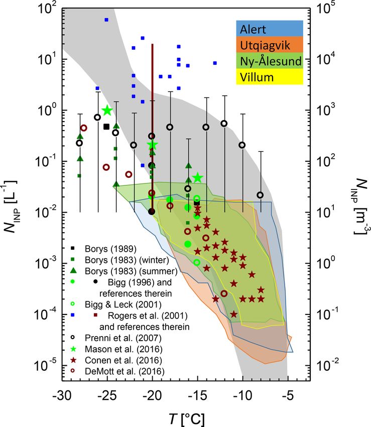
H. Wex et al.: Annual Arctic INP concentrations                                                                             5295

supermicron size range were the most efficient INPs. During        the tropics, could be expected to be linked to a lack of bio-
sampling phases from March until mid-May, when grounds             genic INPs in the Arctic due to sparse biological activity.
were covered in snow and ice, number concentrations of the         However, it is known that biogenic INPs are contained in
supermicron INPs were lower than those in late May by up to        seawater (Schnell, 1977) and the oceanic surface microlayer
2 orders of magnitude. The increase in NINP was suggested to       (SML) (Wilson et al., 2015; Irish et al., 2017) and are emit-
originate from open leads in the sea ice and from open tundra.     ted to the atmosphere by sea spray production (DeMott et al.,
Similarly, for a coastal mountain station in northern Norway       2016). An increase in INP concentrations in the SML (Wil-
(at 70◦ N), based on four filters sampled during July, Conen       son et al., 2015) and for the biosphere in general (Schnell
et al. (2016) observed that air masses were enriched in INPs       and Vali, 1976) from equatorial regions towards the poles has
ice active at −15 ◦ C when they had passed over land. An ori-      been observed. Also present in the Arctic are fungi (Fu et al.,
gin of these INPs from decaying leaves was suggested. Irish        2013), lichen, and bacteria (Santl-Temkiv et al., 2018), which
et al. (2019) derived NINP during a ship cruise in the Cana-       could potentially contribute biogenic INPs.
dian Arctic marine boundary layer in summer. They suggest             In the present study, we aimed at increasing the knowl-
that mineral dust contributed more strongly to the observed        edge of Arctic surface concentrations of INPs active in the
INPs than sea spray, with mineral dust particles likely origi-     immersion freezing mode, as described in the following.
nating in the Arctic (Hudson Bay, eastern Greenland, north-        The immersion freezing mode was examined as it has been
west continental Canada).                                          described as the most important heterogenous ice nucle-
   Different substances are known to contribute to atmo-           ation mode in mixed-phase clouds (Ansmann et al., 2009;
spheric INPs, as outlined in a number of review articles           Wiacek et al., 2010; de Boer et al., 2011). No specific mea-
(Szyrmer and Zawadzki, 1997; Hoose and Moehler, 2012;              surement campaign was organized for the examinations de-
Murray et al., 2012; Kanji et al., 2017). In general, it is        scribed herein. Instead, use was made of already existing fil-
known that NINP increases roughly exponentially with de-           ter samples. Besides for deriving temperature spectra of NINP
creasing T , although at higher T steep increases may be           for 104 filter samples (Sect. 3.1), we also determined pos-
observed, followed by a weaker increase or even a plateau          sible sources for INPs that are ice active at high T for se-
region down to roughly −20 ◦ C (as seen in, e.g., Petters          lected samples. For that, correlations between NINP and some
and Wright, 2015; O’Sullivan et al., 2018; Creamean et al.,        chemical compounds were made (Sect. 3.2.1), and an anal-
2018b). Ice nucleation at higher T is typically related to         ysis was done concerning possible regions of origin of INPs
macromolecules from biogenic entities as bacteria, fungal          that are ice active at high T (Sect. 3.2.2) for a selection of
spores, lichen, pollen, and marine biota. These ice-active         samples. The results will also be discussed in light of litera-
macromolecules nucleate ice from just below 0 ◦ C down to          ture data (Sect. 4).
roughly −20 ◦ C (Murray et al., 2012; Kanji et al., 2017;
O’Sullivan et al., 2018). Biogenic INPs typically occur in low
concentrations in the atmosphere, but nevertheless, at remote      2   Measurements
marine locations such as the Southern Ocean, where NINP is
generally low, marine biogenic INPs might make up a large          Quartz-fiber filters were sampled regularly at the four Arctic
fraction or even the entire INP population (Burrows et al.,        measurement stations of Alert, Ny-Ålesund, Utqiaġvik, and
2013; McCluskey et al., 2018a). At less remote locations, the      Villum Research Station (VRS) during the past years. Fig-
majority of atmospheric INPs consist of mineral dust parti-        ure 1 shows the locations of these four stations, which are
cles originating from deserts or soils. Pure mineral dust parti-   all in close proximity to the ocean (< 3 km). A portion of
cles of atmospherically relevant sizes typically are ice active    the filters was provided for the analysis presented herein. In
below −15 ◦ C (Murray et al., 2012; Kanji et al., 2017) or         the following, some detail will be given on these four dif-
even below −20 ◦ C (Augustin-Bauditz et al., 2014) and, with       ferent stations, including the filter handling, and on the mea-
the abovementioned exception of remote marine locations,           surement and evaluation method used to obtain INP num-
typically occur at much higher concentrations than biogenic        ber concentrations. We also describe in detail the tempera-
INPs (Murray et al., 2012; Petters and Wright, 2015). How-         ture history of the filters, although it is not yet known with
ever, mineral dust particles might also occur together with        certainty how the temperature during storage will affect INP
biogenic ice-active material (Tobo et al., 2014; O’Sullivan        concentrations. Generally, the filters were kept frozen when-
et al., 2014; Hill et al., 2016), and such a mixed particle        ever possible. Transport from the four institutes where the
acts like a biogenic INP (Augustin-Bauditz et al., 2016) and       samples had been kept to TROPOS was done in insulated
should be attributed to the aforementioned group of biogenic       boxes, together with cooling elements. The shipment was or-
INPs.                                                              ganized such that transport was fast (1–3 d) and that upon ar-
   The existence of particularly high fractions of supercooled     rival at TROPOS the temperature in the boxes was still below
water observed in Arctic stratiform clouds, as, e.g., observed     0 ◦ C. At TROPOS, samples were again stored at −18 ◦ C until
in Costa et al. (2017) in the temperature range above −20 ◦ C      the measurements were done. These measures during storage
in comparison to more convective clouds in midlatitudes and        and transport are precautions, as for biogenic INPs, storage at

www.atmos-chem-phys.net/19/5293/2019/                                               Atmos. Chem. Phys., 19, 5293–5311, 2019
5296                                                                          H. Wex et al.: Annual Arctic INP concentrations

                                                                     ilarly to the other filters, i.e., inserted into the sampler for
                                                                     2 min, but without an airflow through them. They were also
                                                                     stored similarly to the sampled filters at all times. After sam-
                                                                     pling, filters were stored (at room temperature ≈ 20 ◦ C) in
                                                                     their sampling cartridges (wrapped in aluminum foil inside
                                                                     sealed plastic bags) at the Alert station and shipped in card-
                                                                     board boxes (containing five sampling cartridges each) to the
                                                                     Toronto lab at Environment Climate Change Canada where
                                                                     they were stored frozen at < −30 ◦ C. From these filters, a
                                                                     circular piece 47 mm in diameter was shipped to Leipzig for
                                                                     this study.
                                                                        The total sampling area on the filters was
                                                                     17.8 cm × 22.8 cm. For the measurements at TROPOS,
                                                                     described in detail in Sect. 2.5 below, circles with 1 mm
                                                                     diameter were punched out from the samples using sterile
                                                                     biopsy punches and immersed in ultrapure water separately.
                                                                     The volume of air sampled per 1 mm piece of filter differed
                                                                     for the different samples and varied from roughly 270 to
                                                                     540 L.

                                                                     2.2   Ny-Ålesund

Figure 1. The location of the four stations from which filter sam-   Filter sampling in Ny-Ålesund on Svalbard (at 78◦ 550 N,
ples were included herein: Utqiaġvik (red diamond), Alert (yellow   11◦ 550 E; 11 m a.s.l.) is done by the University of Florence,
diamond), VRS (green diamond), and Ny-Ålesund (blue diamond).        Italy. Quartz-fiber filters have been sampled regularly since
                                                                     2010 using a high-volume sampler with quartz microfiber
                                                                     filters (CHMLAB Group QF1 grade, Barcelona, Spain). The
temperatures above 0 ◦ C or even storage under freezing con-         filters were pretreated at 400 ◦ C prior to sampling. The fil-
ditions has been found to reduce their ice activity (Wex et al.,     ters had a diameter of 47 mm, one-quarter of which was pro-
2015; Polen et al., 2016, respectively). In this study, unless       vided for the present study. Sampling duration was 4 d in
mentioned otherwise, all samples from all stations (also in-         2012, and of these filters, 13 sampled from late March un-
cluding field blanks) were treated similarly during all proce-       til the beginning of September were examined in the present
dures. In the next sections, peculiarities of the separate four      study, together with two field blanks. The total air volume
stations are described, followed by details of the measure-          collected on each filter was roughly 200 m3 . Each circular
ments and their evaluation.                                          1 mm filter piece used for the analysis sampled particles from
                                                                     roughly 130 L. Once sampled, filters were stored in a freezer
2.1    Alert                                                         at the Italian base in Ny-Ålesund and then shipped to Italy
                                                                     via cargo. At the home university, they were then stored in a
A custom-built high-volume aerosol sampler was used at               cold room at −20 ◦ C.
the Dr. Neil Trivett Global Atmosphere Watch Observa-
tory in Alert, Canada (82◦ 300 N, 62◦ 220 W; 210 m above             2.3   Utqiaġvik (formerly known as Barrow)
sea level, a.s.l.), to collect 38 samples between April 2015
and April 2016. The sampler is installed at a walk-up deck           Filter sampling in Utqiaġvik, Alaska (at 71◦ 180 N,
about 4 m above the ground. The flow rate is approxi-                156◦ 460 W; 11 m a.s.l.), is done by Baylor University,
mately 1.4 m3 min−1 at standard temperature and pressure             US, as described in Barrett and Sheesley (2017). For the
(STP) conditions. Quartz filters (8×10 in; Pall Life Sciences,       present study, quartz-fiber filters were used that had been
Pallflex filters, USA) were pre-fired at 900 ◦ C overnight and       sampled regularly in an annual campaign from June 2012
then shipped to Alert while already loaded on cartridges.            to June 2013 using a high-volume sampler (Tisch Environ-
During transport and storage, the filter-containing cartridges       mental, Cleves, OH, USA). Filters were stored frozen prior
were wrapped with aluminum foil, and they were inside                to and immediately following all sampling. Two rectangular
sealed plastic bags. Sampling time for those filters was ei-         filter pieces (with a lateral length of 1.5 cm) from each of
ther 1 week or 2 weeks, the latter being used from August            41 different filters and two field blanks were provided for the
until October (due to operational issues, no filter was sam-         present study. The sampled area of each filter was 399 cm2 .
pled in July). A total of nine field blanks (roughly one every       Sampling on each filter was done for 4 up to 13 d (7 d on
month) were collected. These field blanks were treated sim-          average), collecting particles from a total air volume of

Atmos. Chem. Phys., 19, 5293–5311, 2019                                               www.atmos-chem-phys.net/19/5293/2019/
H. Wex et al.: Annual Arctic INP concentrations                                                                                5297

roughly 14 000 to 51 000 m3 . This yields an air volume of          Frozen fractions (fice ) were then determined as the number
roughly 270 to 1000 L collected on each circular 1 mm filter        of frozen tubes divided by the total number of tubes. Typ-
piece used for the analysis. Prior to sampling, filters were        ically, fresh water to be used in the experiments was taken
pretreated at 500 ◦ C. After sampling, the filters were stored      once a day and stored in a glass bottle. Whenever fresh wa-
in a freezer on-site and transported to the home university in      ter was taken, an experiment was run with this water in the
coolers with cooling elements, where they were then stored          tubes only to ensure that the water was satisfyingly clean.
at −18 ◦ C.                                                         Similarly, experiments were run with field blank filters that
                                                                    had the same history as the samples but without sampling
2.4   Villum Research Station                                       (see the Supplement), and signals from the field blanks were
                                                                    well below those of the sampled filters. A subtraction of the
Villum Research Station (VRS) at Station Nord in northern           signals of the field blank from those of the measurements
Greenland (at 81◦ 360 N, 16◦ 400 W; 24 m a.s.l.) is operated by     was not done. This is justified in a detailed discussion in the
Aarhus University, Denmark (in cooperation with the Dan-            Supplement. The interpretation of the results from the filters
ish Defense, the Arctic Command). Quartz-fiber filters have         presented in this study is the same for both uncorrected and
been sampled regularly since 2008 using a high-volume sam-          background-corrected samples.
pler (DIGITEL Hegnau, Switzerland) and employing weekly
sampling (Bossi et al., 2016). The filters had an exposed           2.6   Deriving NINP
area of 154 cm2 and sampled a total air volume of roughly
5000 m3 . From filters sampled in 2015, a 2 cm diameter piece       Equation (1) was used to derive NINP from the measured fice
was cut from each of the filters and provided for this study.       (Vali, 1971; Conen et al., 2012). This equation accounts for
Due to the large interest in shares of the filters, only samples    the possibility of the presence of multiple INPs in one vial
from 11 different filters, all from different months in 2015        by assuming that the INPs are Poisson distributed. Addition-
and 1 from December 2013, could be used herein. As for all          ally it normalizes the values resulting from the measurement
samples used in this study, from the 2 cm pieces punches of         with the air volume sampled on each 1 mm filter piece. This
1 mm in diameter were cut at TROPOS directly prior to the           yields concentrations of ice-nucleating particles per volume
measurements. The resulting small pieces were then used for         of sampled air.
INP analysis. The area of these 1 mm pieces corresponds to a        NINP = − (ln(1 − fice )) / F · Ap /Af

                                                                                                                              (1)
sample volume of 255 L of air. Prior to sampling in the field,
filters were pretreated at 450 ◦ C. Storage of the filters at VRS   F is the total volume of air drawn through the filter, and Ap
was done in freezers. Filters are transported from Greenland        and Af are the surface area of a single 1 mm filter piece and
to Denmark around three times per year by the Danish Royal          the whole sampled area of the filter, respectively.
Air Force and then shipped to Roskilde, where they were then           The temperature and concentration regions for which data
stored at −18 ◦ C.                                                  were obtained for the different samples depend on a number
                                                                    of factors. The measured value fice is a fraction ranging from
2.5   Freezing device INDA, the Ice Nucleation Droplet              0 to 1. Therefore, NINP , as derived using Eq. (1), can only
      Array                                                         take on a limited range of values. This range is based on the
                                                                    negative natural logarithm of 0.01 and 0.99 (4.6 to 0.01). The
For freezing experiments examining immersion freezing, a            absolute values of NINP then also depend on the volume of
device comparable to one introduced in Conen et al. (2012)          air sampled onto each 1 mm filter piece, i.e., on the volume of
was used, but deploying PCR trays (Hill et al., 2016) instead       air drawn through the filter during the sampling period and on
of separate tubes. The same device had been used in Chen            the relation of the surface area of one filter piece to the total
et al. (2018). From each filter piece that had been shipped         sampled surface area. The volume collected per 1 mm filter
to TROPOS, circles with a diameter of 1 mm were punched             piece was within a factor of 4.5 for all filters (120 to 540 L).
out directly before measurements were done, and each of the         Altogether, the range of NINP that can be obtained herein is
96 wells of a PCR tray was filled with such a filter piece to-      roughly from 2 × 10⁻⁵ to 0.04 L−1 . From this limitation, it
gether with 50 µL of ultrapure water (background measure-           also follows that the range of T for which NINP could be
ments of ultrapure water are given in the Supplement). After        obtained is limited, as it is tied to the concentrations that can
sealing the PCR tray with a transparent foil, it was immersed       be measured. Times with more ice-active INPs show up as
into a bath thermostat such that the water table in the wells       NINP at higher T . The highest T at which ice activity was
was below the surface of the liquid in the thermostat. The          observed was close to −5 ◦ C, as will be shown in the next
bath of the thermostat was then cooled with a cooling rate of       section.
1 K min−1 , and the freezing process was monitored by a cam-           It should also be noted that samples that had less than 60 L
era, taking a picture every 6 s. An LED light source installed      of air volume collected on each 1 mm filter piece were also
below the PCR tray ensured that wells in which the water was        examined, but fice was close to the background and there-
still liquid could be easily distinguished from frozen ones.        fore these samples were not considered in this study. Results

www.atmos-chem-phys.net/19/5293/2019/                                                Atmos. Chem. Phys., 19, 5293–5311, 2019
5298                                                                         H. Wex et al.: Annual Arctic INP concentrations

from background measurements are given in the Supplement.          the back trajectories were only considered back in time until
Measurement uncertainty as shown in this work was derived          an integral amount of 2 mm of precipitation (taken from the
based on Harrison et al. (2016), i.e., following the assump-       information included in the back trajectories) was reached.
tion that the INPs are Poisson distributed between the differ-     This was done as precipitation formation occurs via the ice
ent examined droplets. The first few droplets that freeze in       phase so that precipitation is assumed to lead to a washout of
each experiment therefore show the highest uncertainties.          INPs.

2.7    Using back trajectories and satellite maps
                                                                   3     Results
A more in-depth analysis concerning possible INP source re-
gions was done for a selection of filter samples from each         In the following, NINP derived from filter samples will
measurement station. For that, 5 d back trajectories were cal-     shortly be introduced. A correlation with some available
culated with HYSPLIT (Stein et al., 2015) to determine the         chemical composition data is made. Finally, an analysis of
origin of sampled air masses. These calculations were based        air mass origins is introduced to analyze possible source re-
on GDAS (Global Data Assimilation System) meteorological           gions for INPs that are ice active at high T . A comparison to
data using an hourly time resolution. A new trajectory was         literature data and further discussion of the results are then
started every 6 h during the whole time for which sampling         presented in Sects. 4 and 5, respectively.
was done on the respective filter. Back trajectories were initi-
ated at an altitude of 100 m above the sampling locations, as      3.1    Arctic atmospheric INP concentrations
this altitude still has a high likelihood of being connected to
the ground and as lower elevations are more prone to uncer-        Quartz-fiber filters from the four different Arctic stations
tainties. In the Supplement, these back trajectories are shown     shown in Fig. 1 were analyzed to derive NINP . Figure 2 shows
separately for the selected examined filter samples.               NINP for all different samples separately for the four sam-
    Using these back trajectories, we examined over which          pling locations. Due to the comparably large number of fil-
ground the air masses collected on the filters had passed in       ters analyzed for Alert and Utqiaġvik, separate curves cannot
the 5 d prior to arrival at the measurement station. The aim       be seen easily in Fig. 2. Therefore, Fig. 3 shows time se-
was to see contributions from open land or open water for          ries of NINP for T at −7, −10, −13, and −9.5 ◦ C for Alert,
the different selected filter samples. Therefore, a distinction    Utqiaġvik, Ny-Ålesund, and VRS, respectively. T was cho-
was made between snow, open land, sea ice, and open water.         sen such that NINP could be obtained for the largest possi-
To do so, maps from the Interactive Multisensor Snow and           ble number of all curves (data for the three samples with
Ice Mapping System (IMS) (Helfrich et al., 2007; National-         the lowest NINP are missing for Alert (29 April and 27 May
Ice-Center, 2008, 2008) were used. IMS maps are a compos-          2015 and 4 April 2016), as is the one with the highest NINP
ite product produced by NOAA/NEDIS (National Oceanic               for Utqiaġvik (3 May 2013), indicated by arrows in Fig. 3).
and Atmospheric Administration’s National Environmental            The yellow background shows for which samples an more in-
Satellite Data and Information Service) combining informa-         depth analysis is presented in Sect. 3.2.2. Error bars in Fig. 3
tion on both sea ice and snow cover. Information from 15 dif-      show the 95 % confidence interval.
ferent sources of input is included in the production of these        It is worth noting that once a sample has a comparably
maps (Helfrich et al., 2007). These maps have been provided        high concentration at one T this is generally observed at all
for 20 years. We used the daily Northern Hemisphere maps           T at which measurements are available and vice versa; i.e.,
with a resolution of 4 km (National-Ice-Center, 2008, 2008).       the curves do not intersect much (see Fig. 2). Therefore, the
For each time step we applied nearest-neighbor interpolation       curves shown in Fig. 3 can be used to discuss observed trends
in space and time to find the corresponding satellite coordi-      for INPs that are ice active at high T . It should also be noted
nate along the back trajectory. With that, for each back tra-      that for Ny-Ålesund, data only exist for March until Septem-
jectory, we determined the conditions on the ground during         ber and that for VRS there is mostly only one data point per
the passage of the air mass, i.e., if the ground was covered by    month, if any (no data exist for February, March, and May).
snow or ice or if open water or open land was present. The            In Figs. 2 and 3 it can be seen that in general NINP obtained
resulting information is shown exemplarily in Fig. 4 for the       for the summer months is higher than for the winter months.
filter samples collected in Alert starting 10 June 2015. Using     A decrease in NINP is observed starting in fall (October or
these maps, we counted how often air masses that were col-         November). For months with the lowest observed ice activity,
lected on one filter were above open land or open water while      which are generally winter and early spring months, values
the air mass was below 100 m. (As will be discussed in detail      for NINP were measured down to below −20 ◦ C. From June
in Sect. 3.2.2, for Utqiaġvik, results reported here always re-   until September mostly INPs that were ice active between −5
fer to an upper altitude of 500 m and 10 d back trajectories.)     and −15 ◦ C were detected (see Fig. 2), and for Utqiaġvik and
An altitude restriction was used as we were trying to geo-         VRS such highly ice-active INPs were observed as early as
graphically locate INP sources on the surface. Additionally,       April. These highly ice-active INPs will be the focus of the

Atmos. Chem. Phys., 19, 5293–5311, 2019                                             www.atmos-chem-phys.net/19/5293/2019/
H. Wex et al.: Annual Arctic INP concentrations 5299
Figure 3. Time series of NINP at T of −7, −10, −13, and −9.5 ◦ C
for Alert, Utqiaġvik, Ny-Ålesund, and VRS, respectively. Small ar-
rows in the panels indicate times when values were either below
(for Alert) or above (for Utqiaġvik) the detection limit. The yellow
background shows for which samples a more in-depth analysis is
presented in Sect. 3.2.2. Error bars show the 95 % confidence inter-
val.
next two sections (Sect. 3.2.1 and 3.2.2). Similarly highly
ice-active INPs have been suggested to be biogenic in ori-
gin based on tests such as heat treatment (Hill et al., 2016;
O’Sullivan et al., 2018), which due to the limited available
amount of filter material could not be done in the present
study.
3.2 Sources of INPs
3.2.1 Correlation to chemical composition
Typical NINP values measured in the atmosphere are several
orders of magnitude below total particle number concentra-
tions, and therefore mass concentrations of INPs are so small
that a correlation between bulk chemical composition and
NINP might not be expected, particularly not for the very rare
INPs that are ice active at high T . This is in line with recent
findings for a long-term study of INPs at Cape Verde by Welti
Figure 2. NINP for all samples. Symbol color distinguishes between et al. (2018). There, no correlation between NINP and bulk
data obtained for the different months, while symbol type indicates chemical composition was found for T down to −16 ◦ C for a
the day of the month when sampling started. Curves with particu-
number of different compounds, which included Ca2+ , Na+ ,
larly high and low NINP are explicitly listed in the legend. (The T
and elemental carbon as tracers of continental, marine, and
axis is the same for panels a–c and different for panel d; see values
for T given on the top and bottom of the figure, respectively.) combustion sources, respectively. At a lower T of −25 ◦ C,
www.atmos-chem-phys.net/19/5293/2019/ Atmos. Chem. Phys., 19, 5293–5311, 20195300 H. Wex et al.: Annual Arctic INP concentrations
Table 1. R, R 2 , and p values for linear correlations between NINP
(as shown in Fig. 2) and different bulk chemical properties.
Location Species R R2 p
Utqiaġvik EC −0.36 0.13 0.02
OC −0.04 < 0.01 0.82
fluoride 0.14 0.02 0.41
chloride 0.13 0.02 0.43
nitrite 0.22 0.05 0.19
bromide −0.01 < 0.01 0.98
sulfate −0.12 0.01 0.47
nitrate 0.03 < 0.01 0.86
Ny-Ålesund PM10 −0.36 0.13 0.22
OC −0.39 0.15 0.18
ammonium −0.44 0.20 0.13
K −0.57 0.32 0.04
Mg −0.36 0.13 0.22
nitrite 0.15 0.02 0.62
nitrate −0.16 0.03 0.59
sulphate −0.60 0.36 0.03
Na −0.30 0.09 0.32
Ca −0.50 0.25 0.08
Cl −0.13 0.02 0.68
Figure 4. Exemplary results from the analysis of the IMS maps for MSA 0.18 0.03 0.55
the filter collected in Alert starting 10 June 2015. In both panels, Alert POC+CC 0.59 0.35 0.01
each row (indicated as track number) represents one trajectory go- OC −0.12 0.01 0.62
ing back in time for 5 d, starting from 0 (when sampling took place), EC 0.05 < 0.01 0.84
and displaying 120 separate time steps. The colors indicate the al-
titude of the air mass for the different time steps in panel (a) and
the respective nature of the ground at the location of the air mass in
panel (b). bonate carbon) in Alert. Both POC and CC contain carbon
that pyrolyzes at 870 ◦ C in a pure He stream (Huang et al.,
2006). CC might indicate the presence of soil dust (Huang
Si et al. (2019) recently reported that mineral dust tracers et al., 2006). POC includes some charred carbon formed at
correlated with INPs, which suggests that mineral dust was 550 ◦ C, which is the lower temperature step of the applied
a major contributor to the INP population at that T . Si et al. analysis (EnCan-total-900 method; Huang et al., 2006; Chan
(2018) found that for three coastal sites in Canada a model et al., 2010), and highly oxidized organic compounds and/or
based on K-feldspar as the only INP calculated NINP that high-molecular-weight refractory carbon. Based on previous
fit measurements well at −25 ◦ C, while at −15 ◦ C measure- studies, the POC mass is proportional to the oxygen mass
ments were underpredicted, suggesting a missing source of in organic aerosols (Chan et al., 2010), releasing as carbon
INPs that are active at higher T . In the following we exam- monoxide at 870 ◦ C. POC was observed to form from su-
ine whether there is a correlation between the INPs detected crose and glucose (Huang et al., 2006) and therefore might
in the present study that are ice active at high T and chemical be indicative of biogenic material. This points towards a di-
composition. rection in which more detailed studies should be undertaken
The examined filters pieces were not particularly sam- in the future. In Sect. 5, we will discuss a range of possible
pled for this study and were entirely needed for the above- sources for the observed INPs.
described INP analysis. No dedicated chemical analysis
could be done additionally. But as other parts of most of the 3.2.2 Determination of possible source regions
filters were also used in other studies, some information on
chemical composition was available. This was used to derive Results from the more in-depth analysis concerning possible
the correlations with NINP shown in Fig. 3, i.e., with those INP source regions, based on back trajectories and satellite
INPs that are ice active at high T . Table 1 shows values for maps as described in Sect. 2.7, are presented in the follow-
R, R 2 , and p for linear correlations between NINP and differ- ing. For this analysis, samples were chosen that had been
ent bulk chemical properties. collected in spring, directly before and after the transition
In general, no correlations were found. The only case with from typical winter to typical summer conditions (see yellow
a positive value for R (0.59) and a low value for p (0.01) background in Fig. 3). A total of 17 separate filter samples
was found for POC+CC (pyrolyzed organic carbon and car- were included: 2 for VRS, 4 each for Alert and Ny-Ålesund,
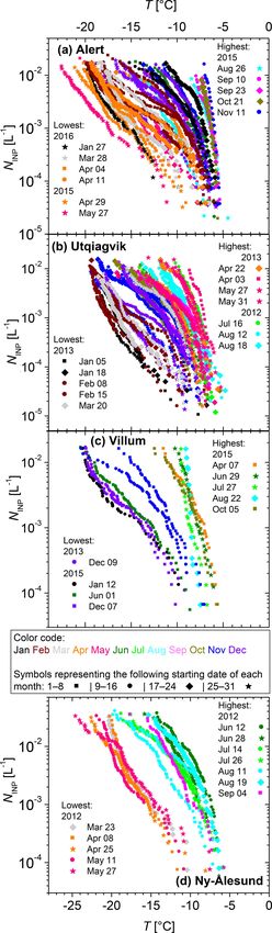
Atmos. Chem. Phys., 19, 5293–5311, 2019 www.atmos-chem-phys.net/19/5293/2019/H. Wex et al.: Annual Arctic INP concentrations 5301
ent types of INP spectra can be distinguished: first, there are
those for which we observed the start of ice activation only at
around −10 ◦ C and which went down to well below −15 ◦ C.
For these, INP spectra and locations are depicted in magenta
or orange. Second, there are INP spectra for which we ob-
served ice nucleation from roughly −5 to above −15 ◦ C. For
these, INP spectra and locations are depicted in greenish col-
ors. The third category was used only for Utqiaġvik for INP
spectra with medium ice activity depicted in blueish. Error
bars shown in Fig. 6 show the 95 % confidence interval.
For Alert, VRS, and Ny-Ålesund, the absence or scarcity
of orange and magenta marks on the maps in Fig. 6 (maps
Figure 5. The number of time steps when air masses were at low on the left in a, b, and c) shows that almost no open land
altitudes and over open land or open water are shown in green and or open water contributed to air masses sampled on the re-
blue, respectively, for different filter samples. The analysis shown spective filters. This is in accordance with the correspond-
was done for altitudes up to 100 m for Alert, Ny-Ålesund, and VRS ing INP spectra, which showed comparably low ice activity.
and up to 500 m for Utqiaġvik. Gray bars in the background in- The magenta locations close to Svalbard for the Alert sam-
dicate the percentage of time the air masses collected on each fil- ple correspond to the sample from 20 May 2015, for which
ter were below that altitude. Triangles indicate samples for which somewhat more ice-active INPs were found than for the sub-
highly ice-active INPs were detected, i.e., for which INP spectra sequent sample from 27 May 2015. For this latter sample, no
were measured at high T (single-colored triangles) and at medium contributions from open land or open water were observed,
T (triangles with yellow interior). The respective INP spectra are
and it is, in fact, the sample with the lowest ice activity ob-
shown in Fig. 6.
served in this study (see Fig. 2). Locations depicted in green-
ish colors potentially contributed INPs that are ice active at
high T . They can be found on open land as well as on open
and 7 for Utqiaġvik. The aim was to see if contributions from water. In connection to filters sampled at Alert or at VRS they
open land or open water were potentially more pronounced show up in north Greenland, on Ellesmere Island (on which
during times when INPs active at high T were observed. Alert is located), in Baffin Bay, and along the southern part
Figure 5 shows the number of time steps when air masses of the west coast of Greenland. Concerning filters sampled
were over open land or open water for the separate filter sam- at Ny-Ålesund, greenish marks show up on Svalbard and the
ples. Additionally, gray bars in the background indicate the adjacent sea.
percentage of time the air masses collected on one filter were The above analysis shows that coastal regions may be par-
below 100 m for Alert, VRS, and Ny-Ålesund. It can already ticularly important as a source for highly ice-active INPs,
be seen that the presence of highly ice-active INPs on a fil- including open waters close to coasts. Indeed, highly ice-
ter is related to air masses that fulfill the above criteria, i.e., active biogenic INPs were found in Arctic surface waters
that traveled over open land or open water at a low altitude. before (e.g., Wilson et al., 2015; Irish et al., 2017). For the
It also can be seen that this was not found for Utqiaġvik. highly ice-active samples collected on Ny-Ålesund on 12 and
Initially, no open land and hardly any open water had been 28 June 2012, the surroundings of the measurement station
found for this site when 5 d back trajectories were used, to- were completely snow free during the times when these sam-
gether with an altitude restriction of 100 m, which means that ples were collected, whereas for all other cases there was
air masses did not travel over open land or open water at alti- at least partial or total snow cover around the stations. In
tudes below 100 m. To check if the length of the back trajec- other words, local terrestrial sources close to the measure-
tory or the chosen maximum altitude influenced our results ment station may also contribute as sources for highly ice-
for Utqiaġvik, an analysis was also done using 10 d back tra- active INPs, as already discussed in Creamean et al. (2018a).
jectories and 500 m as the altitude limit, which is presented in Also, Irish et al. (2019) describe Arctic landmasses to be the
Fig. 5. This extension only resulted in larger percentages of source for observed Arctic INPs (ice active at −15, −20,
time for which the air masses were below this altitude limit. and −25 ◦ C), and these INPs were suggested to be mineral
However, there were still not a large number of time steps dust. On Svalbard, Tobo et al. (2019) found higher atmo-
found for which air masses traveled over open land or open spheric NINP in July than in March, and they additionally
water for Utqiaġvik. We will get back to this again below. described glacial outwash sediments in Svalbard to be highly
Figure 6 shows the spectra of NINP (called INP spectra ice active. This ice activity was assumed to be connected to
for simplicity from now on) for the samples included in this small amounts of organic (likely biogenic) material. Based
analysis (right side) and the locations where the respective air on these findings, Tobo et al. (2019) suggest the higher NINP
masses traveled over open land or open water at altitudes be- in summer to be connected to organic (biogenic) components
low 100 m (or 500 m for Utqiaġvik) (left side). Three differ- in glacially sourced dust. Some coastal regions in the Arctic,
www.atmos-chem-phys.net/19/5293/2019/ Atmos. Chem. Phys., 19, 5293–5311, 20195302 H. Wex et al.: Annual Arctic INP concentrations Figure 6. Panels (a), (b), (c), and (d) each show a map on the left side in which locations are indicated where air masses collected on different filters crossed over open land or open water while being at a low altitude (below 100 m for Alert, Ny-Ålesund, and VRS; below 500 m for Utqiaġvik). Black diamonds indicate the location of the measurement site. (Please note: the maps in c and d are rotated by 90◦ compared to the those in a and b.) The right side shows the INP spectra for the corresponding filters. e.g., the west coast of Greenland together with the region and INPs are likely also emitted from regions with high bi- around Baffin Bay and the Canadian Arctic Archipelago as ological activity. In Sect. 5 we will discuss possible INP well as the area around the Bering Strait and also Svalbard, sources in more detail. are known for their abundance of seabird colonies (Croft For Utqiaġvik, data from seven filters were included in the et al., 2016). These regions partially coincide with regions analysis. Two of them showed INP spectra at comparably low highlighted as possible INP sources in Fig. 6. These regions T , three at medium T , and two at high T . For all types of are known to emit ammonia, which plays a role in new par- INP spectra, no contribution from open land was observed ticle formation in the Arctic (Croft et al., 2016). But clearly, with the back-trajectory analysis. Only minor contributions newly formed particles are not expected to contribute to at- from open water were found for the latter two types, although mospheric INPs at the temperatures examined in this study, the analysis was extended to include 10 d back trajectories, Atmos. Chem. Phys., 19, 5293–5311, 2019 www.atmos-chem-phys.net/19/5293/2019/
H. Wex et al.: Annual Arctic INP concentrations                                                                                 5303

and the maximum altitude up to which air masses were con-
sidered was relaxed to 500 m. Air masses did travel below
100 m, and even more often below 500 m (see Fig. 5 and the
back trajectories for Utqiaġvik and their heights profiles in
the Supplement). However, the transition to filters on which
INPs active at comparably high T was already found to hap-
pen earlier at Utqiaġvik than at the other three measurement
locations towards the end of March. IMS maps almost exclu-
sively identified the ground as sea ice and snow in the regions
that were crossed by the air masses, even until the beginning
of May 2013. And in general, air masses spent more time
over sea ice than over snow (see back trajectories in the Sup-
plement). There has to be a source for highly ice-active INPs
that was not revealed in the analysis done here. Polynyas and
open leads may contribute to explaining this inconsistency.
The resolution of the IMS maps used may be too coarse so
that open water related to polynyas and open leads could have
gone unnoticed.
   While the analysis introduced here shows regions that may
have potentially contributed highly ice-active INPs to the
sampled air masses, it does not make any statement about
other regions. Other regions could potentially be sources, too,
but might have only been crossed by air masses at high alti-
tudes or may not have been crossed at all.
                                                                  Figure 7. Comparison of NINP determined in this study for the Arc-
                                                                  tic with literature data by Petters and Wright (2015) (gray back-
4   Comparison with literature                                    ground), Borys (1983, 1989), Bigg (1996), Bigg and Leck (2001),
                                                                  Rogers et al. (2001), Prenni et al. (2007), Mason et al. (2016), Co-
Figure 7 shows the ranges of NINP observed for the four sta-      nen et al. (2016), and DeMott et al. (2016). Green and brown sym-
tions as shaded areas. Data from the different stations cover     bols represent data from surface-based measurements; black and
a rather similar range. As explained above (Sect. 2.6), NINP      blue represent airborne measurements. For Rogers et al. (2001),
                                                                  brown indicates data they cited from the literature, with the verti-
could only be measured up to some 10−2 L−1 , depending on
                                                                  cal bar indicating the extent of the reported values.
the volume of air sampled onto one 1 mm filter piece. Hence,
the upper concentration limit of our data is determined by
the measurement method. The gray background shows lit-
erature data of NINP determined from precipitation samples        et al., 2001; Prenni et al., 2007; Mason et al., 2016; Co-
collected mostly in North America and Europe (Petters and         nen et al., 2016; DeMott et al., 2016). Not every single data
Wright, 2015). In that data set, samples showing the high-        point from these papers is shown, as Fig. 7 aims to give an
est NINP at T > −20 ◦ C originate from rain and hail sam-         overview of the range of data that exists. Data on Arctic NINP
ples collected in North Carolina (US) and Alberta, Montreal       in general are still scarce, which is particularly true for data
(CA). Some of the INP spectra we detected at the highest T ,      at high T . Also, data scatter over a wide range. The highest
observed particularly in Alert and Utqiaġvik, show values for    values of NINP shown in Fig. 7 originate from one set of air-
NINP that are similar or only about 1 order of magnitude be-      craft measurements made in May (Rogers et al., 2001), while
low data reported in Petters and Wright (2015). At the lowest     a second set of aircraft measurements, taken in September
temperatures at which we detected INP spectra, NINP val-          and October onboard an aircraft flying out of Alaska, agrees
ues are lower than data from Petters and Wright (2015), i.e.,     with our data at the highest T (Prenni et al., 2007). For the
the lowest Arctic NINP , as those we observed in the winter       data taken from Prenni et al. (2007), the reported measure-
months might be below the lowest values observed on conti-        ment uncertainty is shown, which is representative for typical
nents in midlatitudes. It is worth adding that still lower con-   uncertainties for the type of instrumentation used in Rogers
centrations were observed in marine remote locations in the       et al. (2001) and Prenni et al. (2007). Error bars indicate
Southern Ocean (McCluskey et al., 2018a) and for clean ma-        1 standard deviation at the higher end. The lower end is in-
rine air in the northeast Atlantic (McCluskey et al., 2018b).     dicative of the detection limit, and for a substantial fraction of
   Figure 7 shows additional data on Arctic NINP from the lit-    measurements no INPs were detected in Prenni et al. (2007).
erature that were already discussed in the Introduction (Bo-         Going back to Fig. 7, literature data from ground-based
rys, 1983, 1989; Bigg, 1996; Bigg and Leck, 2001; Rogers          measurements that are in the same range of NINP in which

www.atmos-chem-phys.net/19/5293/2019/                                               Atmos. Chem. Phys., 19, 5293–5311, 2019
5304 H. Wex et al.: Annual Arctic INP concentrations we measured are also within the same T range. But besides heights up to levels at which cloud formation is observed. the data from Conen et al. (2016), these data are at the lower Hence, INPs detected by ground-based measurements may end of T that we observed. This also holds for the data from well be able to influence ice formation in clouds, at least dur- DeMott et al. (2016), which were obtained during summer ing times when the cloud layers are coupled to the surface. ship cruises in Baffin Bay and in the central Bering Sea. Compared to previous literature data introduced in this Data shown for Borys (1983) were taken in Ny-Ålesund study, the new long-term data presented here extend the range and Utqiaġvik. A slight tendency towards higher NINP in of Arctic NINP towards higher T . They also clearly show that summer months, compared to winter months, can be seen. Arctic INP concentrations vary throughout the year, with a Similarly, as said in the Introduction, Bigg and Leck (2001) regular presence of INPs that are ice active at T well above found a decreasing trend for NINP at −15 ◦ C from July to −10 ◦ C throughout the summer months at all four terrestrial September. The observed decrease was roughly 1 order of measurement stations. magnitude; however, the scatter from sample to sample was almost as large as that trend. Nevertheless, these data sets are early indications of the annual trend that has very clearly 5 Discussion been found in the present study. Concerning possible sources for INPs, Bigg (1996) as- The annual cycle observed for NINP in this study is not in sumed that mainly oceanic sources contributed to the ob- tune with what is known for particle number concentrations served INPs, with only a weak contribution from land. Bigg and size distributions occurring across the Arctic (Tunved and Leck (2001) discussed a marine origin of at least some et al., 2013; Nguyen et al., 2016; Freud et al., 2017). This of the INPs they analyzed. These latter two studies were ship is not too surprising: recent studies, including Arctic loca- based. The land-based study by Conen et al. (2016) showed tions, found that a large fraction of INPs are supermicron in INPs that were ice active at higher T than those observed in size (Mason et al., 2016; Si et al., 2018; Creamean et al., Bigg (1996) and Bigg and Leck (2001). Conen et al. (2016) 2018a), while the majority of particles are in the submicron traced these INPs back to terrestrial contributions, possi- size range. bly decaying leaves. During aircraft measurements, Rogers Concerning the annual Arctic aerosol cycle, there is a max- et al. (2001) identified some INPs as mineral dust particles imum in particle number concentrations in early spring, be- and others as containing low-molecular-weight components. fore precipitation sets in, caused by accumulating anthro- These latter might have been connected to biogenic INPs. pogenic pollution known as Arctic haze (Shaw, 1995). NINP These different studies report very diverse NINP . In these values are low during that time of the year, which might in- studies, different instrumentation was used and sometimes dicate that anthropogenic pollution does not contribute to at- different ice nucleation mechanisms were probed. Also, in- mospheric INPs, at least in the T range examined in this strumental limitations typically determine the ranges of T study. This is in line with the observation that Arctic haze and NINP that can be probed. All of this might add to the particles are not efficient INPs (Borys, 1989) and also with diversity in the data. But, as can be seen in Fig. 3, a differ- a recent study showing that anthropogenic pollution did not ence of up to 2 orders of magnitude in NINP was measured contribute to INPs in very polluted air in Beijing (Chen et al., between winter and summer for a single temperature in our 2018). It is also in agreement with observations by Hartmann data set. Therefore, the diversity in NINP reported in previous et al. (2019) based on ice cores from Svalbard and Greenland, studies will also originate from different times of the year who found that NINP in the Arctic did not increase over the when these studies were conducted. past 500 years (from roughly 1480 to 1990), while tracers for All of our samples were collected on land, and regions anthropogenic pollution did increase markedly. that showed up as possible sources for highly ice-active INPs The formation of Arctic haze is related to the fact that dur- in Fig. 6 were on or close to land. While, as said above ing winter months, air masses from midlatitudes can trans- (Sect. 3.2.2), other regions cannot be excluded as sources, port aerosol particles into the Arctic (Heidam et al., 1999; it will be interesting to see in the future if NINP values de- Stohl, 2006). In contrast, in the summer months the Arctic tected further away from terrestrial sources will consistently lower atmosphere is effectively isolated and the transport of be lower than those obtained on land. atmospheric aerosol particles into the Arctic is low (Heidam Concerning an influence of INPs emitted from the ground et al., 1999; Stohl, 2006). Hence, the increase in NINP ob- at higher altitudes, Herenz et al. (2018) recently compared served here in late spring and summer has to originate from aerosol particle number size distributions (PNSDs) measured Arctic sources, including local ones situated close to the mea- on the ground and during overflights at different heights in surement site. May 2014 in Tuktoyaktuk (Northwest Territories of Canada Once Arctic haze is removed by precipitation in spring on the Arctic Ocean). PNSDs measured on the ground and (Browse et al., 2012), Arctic particles are mostly newly at heights up 1200 m were generally similar, while PNSDs formed particles in the size range up to 100 nm (Lange et al., obtained at higher altitudes were clearly different. There- 2018), originating from gaseous precursors (Engvall et al., fore, atmospheric aerosol, including INPs, can be similar at 2008; Leaitch et al., 2013; Croft et al., 2016; Wentworth Atmos. Chem. Phys., 19, 5293–5311, 2019 www.atmos-chem-phys.net/19/5293/2019/
You can also read