Mapping Spatial Distribution and Biomass of Intertidal Ulva Blooms Using Machine Learning and Earth Observation - NUI Galway
←
→
Page content transcription
If your browser does not render page correctly, please read the page content below
ORIGINAL RESEARCH
                                                                                                                                               published: 13 April 2021
                                                                                                                                      doi: 10.3389/fmars.2021.633128

                                            Mapping Spatial Distribution and
                                            Biomass of Intertidal Ulva Blooms
                                            Using Machine Learning and Earth
                                            Observation
                                            Sita Karki 1,2 , Ricardo Bermejo 1 , Robert Wilkes 3 , Michéal Mac Monagail 1 , Eve Daly 1 ,
                                            Mark Healy 4 , Jenny Hanafin 2 , Alastair McKinstry 2 , Per-Erik Mellander 5 , Owen Fenton 5
                                            and Liam Morrison 1*
                                            1
                                              Department of Earth and Ocean Sciences, School of Natural Sciences and Ryan Institute, National University of Ireland
                                            Galway, Galway, Ireland, 2 Irish Centre for High-End Computing, National University of Ireland Galway, Galway, Ireland,
                                            3
                                              Environmental Protection Agency (EPA), Castlebar, Ireland, 4 Department of Civil Engineering, School of Engineering
                                            and Ryan Institute, National University of Ireland Galway, Galway, Ireland, 5 Teagasc Agricultural Catchments Programme,
                                            Teagasc Environment Research Centre, Wexford, Ireland

                            Edited by:      Opportunistic macroalgal blooms have been used for the assessment of the ecological
                      Ricardo A. Melo,
         University of Lisbon, Portugal
                                            status of coastal and estuarine areas in Europe. The use of earth observation (EO)
                        Reviewed by:
                                            data sets to map green algal cover based on a Normalized Difference Vegetation
                            Hanzhi Lin,     Index (NDVI) was explored. Scenes from Sentinel-2A/B, Landsat-5, and Landsat-8
        University of Maryland Center
                                            missions were processed for eight different Irish estuaries of moderate, poor, and bad
 for Environmental Science (UMCES),
                         United States      ecological status using European Union Water Framework Directive (WFD) classification
                         José M. Rico,      for transitional water bodies. Images acquired during low-tide conditions from 2010 to
           University of Oviedo, Spain
                                            2018 within 18 days of field surveys were considered. The estimates of percentage
                 *Correspondence:
                        Liam Morrison
                                            coverage obtained from different EO data sources and field surveys were significantly
           liam.morrison@nuigalway.ie       correlated (R2 = 0.94) with Cohen’s kappa coefficient of 0.69 ± 0.13. The results showed
                                            that the NDVI technique could be successfully applied to map the coverage of the
                   Specialty section:
         This article was submitted to
                                            blooms and to monitor estuarine areas in conjunction with other monitoring activities
          Marine Ecosystem Ecology,         that involve field sampling and surveys. The combination of wide-spread cloud-coverage
               a section of the journal
                                            and high-tide conditions provided additional constraints during the image selection. The
          Frontiers in Marine Science
                                            findings showed that both Sentinel-2 and Landsat scenes could be utilized to estimate
       Received: 24 November 2020
          Accepted: 22 March 2021           bloom coverage. Moreover, Landsat, because of its legacy program, can be utilized
           Published: 13 April 2021         to reconstruct the blooms using historical archival data. Considering the importance
                             Citation:      of biomass for understanding the severity of algal accumulations, an artificial neural
        Karki S, Bermejo R, Wilkes R,
      Monagail MM, Daly E, Healy M,
                                            networks (ANN) model was trained using the in situ historical biomass samples and the
              Hanafin J, McKinstry A,       combination of radar backscatter (Sentinel-1) and optical reflectance in the visible and
         Mellander P-E, Fenton O and
                                            near-infrared (NIR) regions (Sentinel-2) to predict the biomass quantity. The ANN model
   Morrison L (2021) Mapping Spatial
Distribution and Biomass of Intertidal      based on multispectral imagery was suitable to estimate biomass quantity (R2 = 0.74).
Ulva Blooms Using Machine Learning          The model performance could be improved with the addition of more training samples.
               and Earth Observation.
           Front. Mar. Sci. 8:633128.
                                            The developed methodology can be applied in other areas experiencing macroalgal
    doi: 10.3389/fmars.2021.633128          blooms in a simple, cost-effective, and efficient way. The study has demonstrated that

Frontiers in Marine Science | www.frontiersin.org                                  1                                             April 2021 | Volume 8 | Article 633128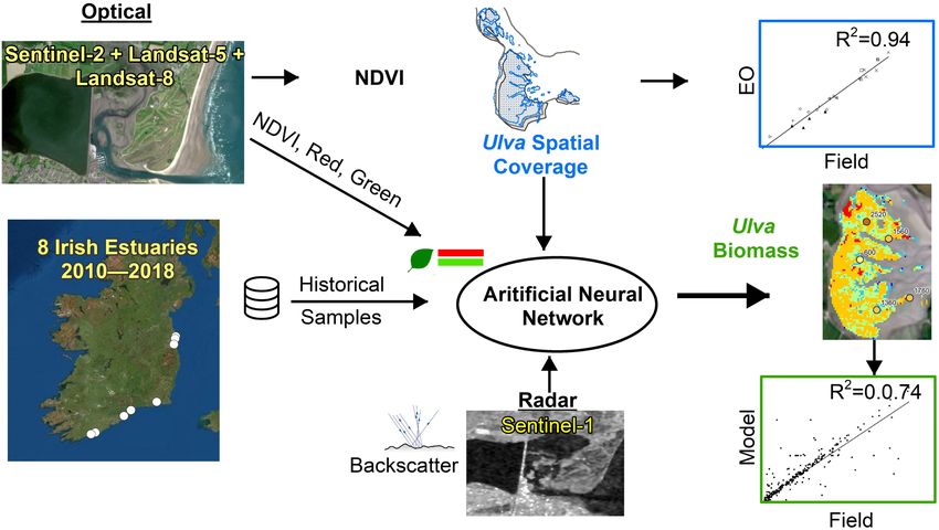
Karki et al.                                                                                                           Earth Observation for Mapping Blooms

  GRAPHICAL ABSTRACT | Overall research workflow showing data types, study area, model development and biomass results.

                                            both the NDVI-based technique to map spatial coverage of macroalgal blooms and
                                            the ANN-based model to compute biomass have the potential to become an effective
                                            complementary tool for monitoring macroalgal blooms where the existing monitoring
                                            efforts can leverage the benefits of EO data sets.
                                            Keywords: Sentinel-1/2, Landsat, earth observation, macroalgal blooms, Ulva, green tides, biomass computation,
                                            artificial neural network

HIGHLIGHTS                                                                        and has obscured the magnitude of degradation in estuarine and
                                                                                  coastal environments (Lotze et al., 2006; Airoldi and Beck, 2007).
 - Mapped green Ulva blooms across eight coastal                                      Estuarine and coastal waters worldwide have been facing the
   areas of Ireland.                                                              problem of eutrophication and macroalgal blooms (Teichberg
 - Bloom extent mapped using Normalized Difference                                et al., 2010). In Europe, eutrophication is considered one of the
   Vegetation Index delineation.                                                  main threats for aquatic ecosystems (Airoldi and Beck, 2007;
 - Developed artificial neural networks (ANN) model to                            Hering et al., 2010). This process is directly linked with nutrient
   compute bloom biomass.                                                         over-enrichment because of increasing anthropogenic nutrient
 - The biomass model utilized optical, radar, and in situ data                    loadings, which significantly increased after the generalized use
   from field surveys.                                                            of industrial fertilizers following the second world war (Cloern,
 - Developed technique could be used in conjunction with                          2001; Lotze et al., 2006; Diaz and Rosenberg, 2008). Due to
   traditional monitoring.                                                        the hydrological and ecological characteristics of estuaries, they
                                                                                  are particularly susceptible to over-enrichment of nutrients and
                                                                                  other pollutants from anthropogenic activities (Sfriso et al.,
INTRODUCTION                                                                      1992; Eyre and Ferguson, 2002). A clear sign of nutrient
                                                                                  enrichment and environmental degradation in estuaries is the
Estuarine and coastal areas play a crucial socio-economic,                        development of opportunistic macroalgal blooms and the loss
biological, and environmental role as these environments provide                  of seagrass meadows (Valiela et al., 1997; Teichberg et al., 2010;
multiple ecosystem goods and services, making them some of                        Bermejo et al., 2019a). Considering the common usage of the
the most valuable ecosystems on earth (Costanza et al., 1997;                     terms, macroalgal bloom and seaweed tides, these are used
Donkersloot and Menzies, 2015; Norton et al., 2018). Due to                       interchangeably in the present paper.
their high value, these areas have been focal points of human                         Macroalgal blooms undermine the ecosystem services that
settlement and resource exploitation (Lotze et al., 2006), resulting              estuaries provide, and affect ecosystem functioning (Smetacek
in a long history of over-exploitation, habitat transformation,                   and Zingone, 2013). As in other parts of the world, some
and pollution. This legacy has undermined ecological resilience                   Irish estuaries contained large green tides in recent years

Frontiers in Marine Science | www.frontiersin.org                             2                                         April 2021 | Volume 8 | Article 633128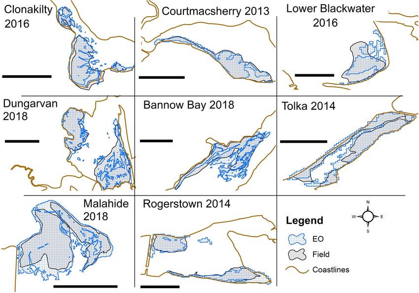
Karki et al.                                                                                                    Earth Observation for Mapping Blooms

(EPA, 2006; Ní Longphuirt et al., 2016; Wan et al., 2017). A recent         et al., 2006; Nezlin et al., 2007). Similarly, the application of
Environmental Protection Agency (EPA) report (EPA, 2019)                    earth observation (EO) satellite data to assess the severity and
has found that transitional waters (i.e., estuaries and coastal             extension of algal blooms in coastal environments has grown
lagoons) in Ireland have poorer water quality when compared                 in recent years (Cristina et al., 2015; Xing and Hu, 2016; Zhang
with other water typologies (i.e., groundwater, rivers, lakes, and          et al., 2019). With the continued development of technology,
coastal waters), with only 38% of water bodies in good or better            unmanned aerial vehicles (UAV) are also being used to monitor
ecological status.                                                          green tides and seaweed blooms in marine environments (Xu F.
    The EU Water Framework Directive (WFD) 2000/60/EC                       et al., 2017; Bermejo et al., 2019b; Taddia et al., 2019; Jiang
(European Commission, 2000) and Marine Strategy Framework                   et al., 2020). Remote sensing methods have been shown to
Directive (MSFD) (2008/56/EC; European Commission, 2008)                    provide reasonable estimates of the algal coverage on the ground
are two of the most ambitious initiatives to prevent further                (Hernandez-Cruz et al., 2006; Nezlin et al., 2007), but with
deterioration of water bodies and associated ecosystems (Wan                the availability of EO data sets with higher temporal, spatial,
et al., 2017; Boon et al., 2020). These directives represent a change       and spectral resolution, further improvement and development
in the scope of water management from the local to the basin scale          can be attained.
(Apitz et al., 2006). They are based on an ecological approach                 Different techniques such as image thresholding (Cavanaugh
rather than a traditional physicochemical assessment (European              et al., 2010, 2011; Cui et al., 2012; Bell et al., 2015), visual
Commission, 2000). This more recent approach is more holistic               interpretation (Donnellan and Foster, 1999; Gower et al., 2006;
since it puts the ecosystem at the center of management decisions           Pfister et al., 2017), supervised classification (Volent et al., 2007;
by considering ecology and biology at a larger scale (e.g., the             Casal et al., 2011; Bermejo et al., 2020), and unsupervised
whole river basin or adjacent coastal area) (Borja, 2005). Both             classification (Fyfe et al., 1999; Duffy et al., 2018) have been used
directives require that coastal areas are periodically monitored            in vegetation mapping in coastal and estuarine areas. Among
to assess their achievement of “Good Ecological Status” and                 the thresholding techniques, band ratios, vegetation indices,
“Good Environmental Status” as per WFD and MFSD targets,                    density, and biomass are commonly used (Richards, 2013),
respectively. The large expansion in monitoring required by the             whereas for supervised classification, spectral angle mapper
WFD and MFSD has created pressure from governments on                       and maximum likelihood classifications are more conventional
their regulatory agencies to reduce the costs of monitoring while           approaches (Schroeder et al., 2019). Regarding classification,
maintaining coverage and effectiveness (Borja and Elliott, 2013;            ground-truth data are used for supervised classification, whereas
Carvalho et al., 2019).                                                     such information is not utilized for unsupervised classification.
    Marine macrophytes, including macroalgae and angiosperms                For both classification types, the results need to be validated
such as saltmarsh and seagrass communities, are biological                  with ground-truth data. Despite its simplicity, one of the
quality elements used to monitor and assess the ecological status           disadvantages of supervised as well as the unsupervised
of transitional and coastal waters for the WFD (e.g., Scanlan               classification is that it results in errors due to digital noise and
et al., 2007; Wells et al., 2007; Bermejo et al., 2012, 2013). Across       these must be removed carefully (Schroeder et al., 2019). Unlike
the EU, monitoring of opportunistic macroalgal blooms is used               classification methods, the image threshold is determined based
to assess the ecological status (Scanlan et al., 2007; Wan et al.,          on the ground-truth data or a validation is performed to check
2017), based on the relative coverage and biomass abundance                 the effectiveness of the threshold.
of opportunistic macroalgae (Wilkes et al., 2018). Monitoring of               Many machine learning-based studies applying aerial or
coastal and estuarine environments can be demanding in terms                remote sensing imagery rely on the greenness of the imagery
of time, labor, costs, and sometimes can pose significant logistical        to map green tides. Although this technique is effective, some
challenges (European Commission, 2008) such as coordination                 areas of the bloom could likely be underestimated, as the
of field equipment, survey procedures, means of transportation,             technique cannot easily delineate the bloom in its entirety.
field crew, and safety. The gathering of this information in muddy          This unreliability results as the technique does not account for
environments, especially the mapping of macroalgal blooms,                  the spectral information available in the near-infrared (NIR)
can present several impediments as it frequently requires the               region where plants exhibit the majority of the photoactivity
use of specialized vehicles such as hovercrafts, or can be very             such as reflection (Tucker and Sellers, 1986). The Normalized
labor intensive. Although these field surveys are systematic and            Difference Vegetation Index (NDVI) is a proxy for vegetation
provide high-quality data regarding spatial coverage and biomass,           health and greenness, and its value ranges from −1 to 1, where
the cost of such works could range from medium to high                      higher value corresponds to the healthy vegetation and lower
(Scanlan et al., 2007).                                                     values correspond to the lack of vegetation (D’Odorico et al.,
    Remote sensing can offer an affordable complementary                    2013; Ke et al., 2015; Zhu and Liu, 2015; Zhang H. K. et al.,
solution to field-based environmental monitoring. Remote                    2018). Since the NDVI technique uses the NIR bands, which
sensing data sets can be freely available, provide wide spatial             are not visible to the naked eyes, it can detect the signature
and temporal coverage, and easily allow methodological                      of vegetation that can go undetected when only visible green
standardizations and comparability. A conventional remote                   bands are used. Although there are numerous other vegetation
sensing technique such as aerial photography has been applied               indices (Silleos et al., 2006; Bannari et al., 2009; Xue and Su, 2017)
to map seagrass and macroalgal distribution in coastal and                  used, including Enhanced Vegetation Index [EVI, primarily
estuarine environments (Jeffrey et al., 1995; Hernandez-Cruz                for Moderate Resolution Imaging Spectroradiometer (MODIS)],

Frontiers in Marine Science | www.frontiersin.org                       3                                        April 2021 | Volume 8 | Article 633128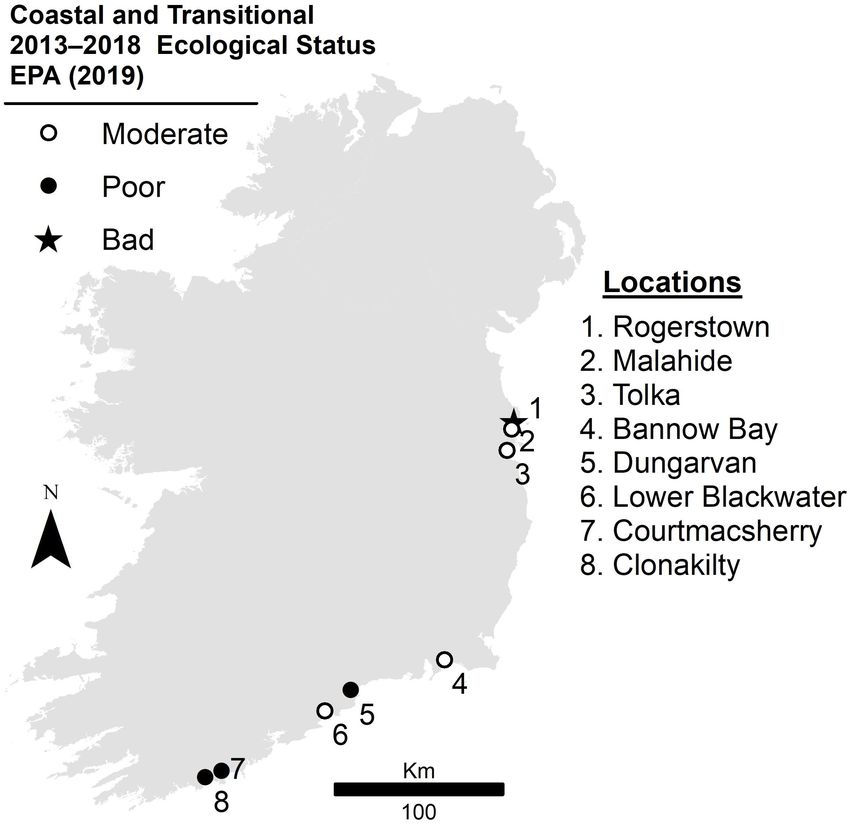
Karki et al.                                                                                                      Earth Observation for Mapping Blooms

Maximum Chlorophyll Index [MCI, primarily for MEdium                           to predict the biomass of Ulva blooms. The benefit ANN
Resolution Imaging Spectrometer (MERIS)], and Floating Algae                   offers over the traditional linear regression-type approach is the
Index (FAI), NDVI was employed in the present study primarily                  ability to model non-linear relationships (Huang, 2009; Karlaftis
because it incorporates the visible and NIR bands at 10 m                      and Vlahogianni, 2011). An ANN offers the potential to deal
resolution which are available in Sentinel-2. Additionally, indices            with a large number of training samples and model complex
developed for detecting vegetation or chlorophyll in aquatic                   relationships taking advantage of multiple input variables
conditions such as FAI and MCI are not applicable in the current               (Bourquin et al., 1998). Unlike other models, ANN offers the
context as macroalgal blooms are being mapped on tidal flats.                  scope for future additional optimization, by the inclusion of
Other studies (Siddiqui and Zaidi, 2016; Siddiqui et al., 2019;                more samples which in turn increases the robustness (Alwosheel
Taddia et al., 2019) have used NDVI and similar vegetation                     et al., 2018). Therefore, the addition of more samples and the
indices for mapping seaweed, but these studies mainly focused                  consideration of further variables provide a learning opportunity
on seaweed immersed in the water. For the studies involving                    to the ANN model which improves predictability over time
seaweed species in water, data sets from ocean color sensors                   (Nadikattu, 2017). These neural networks when adequately
have been used to obtain estimates of chlorophyll present in the               trained can model the natural environment making them suitable
water (Gower et al., 2006, 2008). Considering the size of the                  to big-data applications such as remote sensing. Due to these
estuaries and the need to map these blooms at a higher spatial                 scalable and expandable qualities, the ANN-based technique
resolution, ocean color sensor-based techniques are not relevant               was adopted in the current study. Despite numerous benefits,
to many estuaries globally. Recent studies have shown that NDVI                there are some drawbacks of ANN which can be considered
can be successfully used for mapping biomass and density of                    a “black box” because of its complex algorithms (Dayhoff and
intertidal macroalgae (Conser and Shanks, 2019; Praeger et al.,                DeLeo, 2001; Zhang Z. et al., 2018). In addition, machine
2020; Salarux and Kaewplang, 2020).                                            learning techniques require a comparatively large number of
    The assessments of the algal blooms are usually accomplished               training samples, which may be difficult for smaller scale
by comparing spatial coverage, but biomass can provide greater                 studies. More importantly, the requirement of robust computing
insights about the severity of the blooms (Scanlan et al., 2007;               and programming platforms frequently discourages quick and
Rossi et al., 2011; Xiao et al., 2019). Furthermore, biomass results           easy implementation.
are more helpful for allocating resources and adopting mitigation                 The primary goal of the current study was to evaluate remote
measures. Despite the usefulness of biomass mapping, there are                 sensing as a supplementary tool for the monitoring of macroalgal
minimal studies that focus on mapping biomass using remote                     blooms in Irish estuaries, where the presence of higher cloud
sensing data sets (Hu et al., 2017; Xiao et al., 2017, 2019). Most             coverage places an additional constraint. In this study, macroalgal
of these studies relied on reflectance computed in the laboratory              bloom mapping based on satellite imagery was compared with
environment in order to develop the biomass model. Those                       in situ mapping for ground-truthing and validation purposes.
models were later used to generate biomass using the data from                 The potential of machine learning methodologies was explored
the MODIS optical sensor. Ocean color sensors such as MODIS                    to map the biomass distribution since the higher resolution of the
are ineffective in mapping bloom patches that are smaller than                 newer sensors, such as Sentinel-2 with 5-day revisit time and 10 m
a few hundred meters in size due to their coarse resolution of                 spatial resolution, accompanied by the greater size of the data,
500 m (Karki et al., 2018). Also, considering the spatial extent of            demands robust computing resources. The integration of these
the estuarine areas, it is essential to use remote sensing data with           approaches in EO can take advantage of the recent technological
greater spatial resolution that can discriminate between various               advances in the field of data science and artificial intelligence
magnitudes of biomass on the tidal flats.                                      (Ali et al., 2015). To address this challenge, the potential of
    In addition to optical sensors, application of radar, for                  an ANN was explored using the information extracted from
example, Advanced Land Observing Satellite-1 (ALOS) PALSAR                     Sentinel-1 radar backscatter and Sentinel-2 optical reflectance.
for biomass estimation, at larger scales such as in forestry is                The historical biomass data collected from field surveys were
common (Jha et al., 2006; Le Toan et al., 2011; Hame et al.,                   combined with the data obtained from the EO to develop
2013); however, its application can be explored at a finer scale for           the biomass model.
algal biomass estimation. In recent years, there have been many
successful applications of Sentinel-1 technologies for biomass
monitoring (Ndikumana et al., 2018; Periasamy, 2018; Crabbe                    MATERIALS AND METHODS
et al., 2019) including those combining radar and optical data sets
(Chang and Shoshany, 2016; Laurin et al., 2018; Navarro et al.,                Study Area
2019; Wang et al., 2019) or using radar for bloom forming Ulva                 The current research was conducted on eight estuarine areas
species (Geng et al., 2020). The application of machine learning               most affected by macroalgal blooms across the Republic of
in the field of macroalgal blooms is increasing as demonstrated                Ireland (Figure 1): (a) Clonakilty, Co. Cork (3,465,900 m2 ); (b)
by recent studies (Zavalas et al., 2014; Kotta et al., 2018; Qiu et al.,       Courtmacsherry, Co. Cork (4,471,200 m2 ); (c) Lower Blackwater
2018; Liang et al., 2019; Kim et al., 2020).                                   Estuary, Co. Waterford (2,873,700 m2 ); (d) Dungarvan, Co.
    Although the application of NDVI is conventional, the present              Waterford (12,399,300 m2 ); (e) Bannow Bay, Co. Wexford
study aims to optimize the benefit of NDVI combined with                       (9,848,700 m2 ); (f) Tolka, Co. Dublin (1,135,917 m2 ); (g)
the application of radar and artificial neural networks (ANN)                  Malahide, Co. Dublin (4,075,200 m2 ); and (h) Rogerstown, Co.

Frontiers in Marine Science | www.frontiersin.org                          4                                       April 2021 | Volume 8 | Article 633128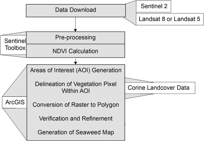
Karki et al.                                                                                                                    Earth Observation for Mapping Blooms

    FIGURE 1 | Map of Ireland showing eight estuarine areas considered in this study with their ecological status based on the study conducted from 2013 to 2018
    (EPA, 2019).

Dublin (4,488,300 m2 ). These areas show a moderate, poor, or                          Clonakilty), and only Bannow Bay had conspicuous seagrass
bad ecological status as assessed for the WFD, parameters driving                      meadows present. Bannow Bay primarily includes intertidal
status included loss of seagrass meadows, general physico-                             zones with predominant macroalgal growth, and the distinction
chemical properties, or the development of large macroalgal                            between seagrasses and Ulva was not conducted because of
blooms (EPA, 20191 ). Although there were different numbers of                         the interspersed, or sometimes negligible, growth of seagrasses
estuaries in each category (moderate: 4; poor: 3; and bad: 1),                         among the macroalgal blooms. Apart from the practical reasons,
standard field surveying techniques were conducted regardless                          green algae and seagrasses are difficult to separate from each
of their status. Consistent with the field protocol, identical EO                      other at the current spectral and spatial signature (Kutser
mapping techniques were also applied. It was important to                              et al., 2020). Since the discrimination between seagrasses and
include a varied range of ecological status conditions in this study                   macroalgae is not possible with Sentinel-2, the study aims to
to make sure that the proposed technique for mapping blooms                            develop a methodology so that field validation can be performed
was not limited to a narrow set of environmental conditions.                           where substantial levels of macroalgal growth occur and any
    In this study, seaweed blooms resembling terrestrial                               potential false positive incidences due to the presence of
vegetation present in the estuaries and tidal flats, excluding                         seagrasses can be verified. This is an example of field monitoring
the salt marshes, were mapped during the low tides. These algal                        and EO complementing each other, reducing logistical and
patches must be mapped during the low tide condition when                              human resource costs, and enhancing environmental quality
there is no water above them. It is crucial to note that estuaries in                  assessment. Seagrasses in Bannow Bay are routinely monitored
Ireland are intertidal in nature, and blooms present in the tidal                      and mapped as a part of obligations under the WFD and the data
flat region may not have water above them except during high                           confirm no risk of false observations from the EO mapping.
tide conditions. In six of the eight sampling locations, seagrass
meadows were absent, or their presence was negligible (i.e.,                           Field Survey
                                                                                       In Ireland, as well as in other cold-temperate regions,
1
    www.catchments.ie                                                                  the maximum development or peak of macroalgal

Frontiers in Marine Science | www.frontiersin.org                                  5                                             April 2021 | Volume 8 | Article 633128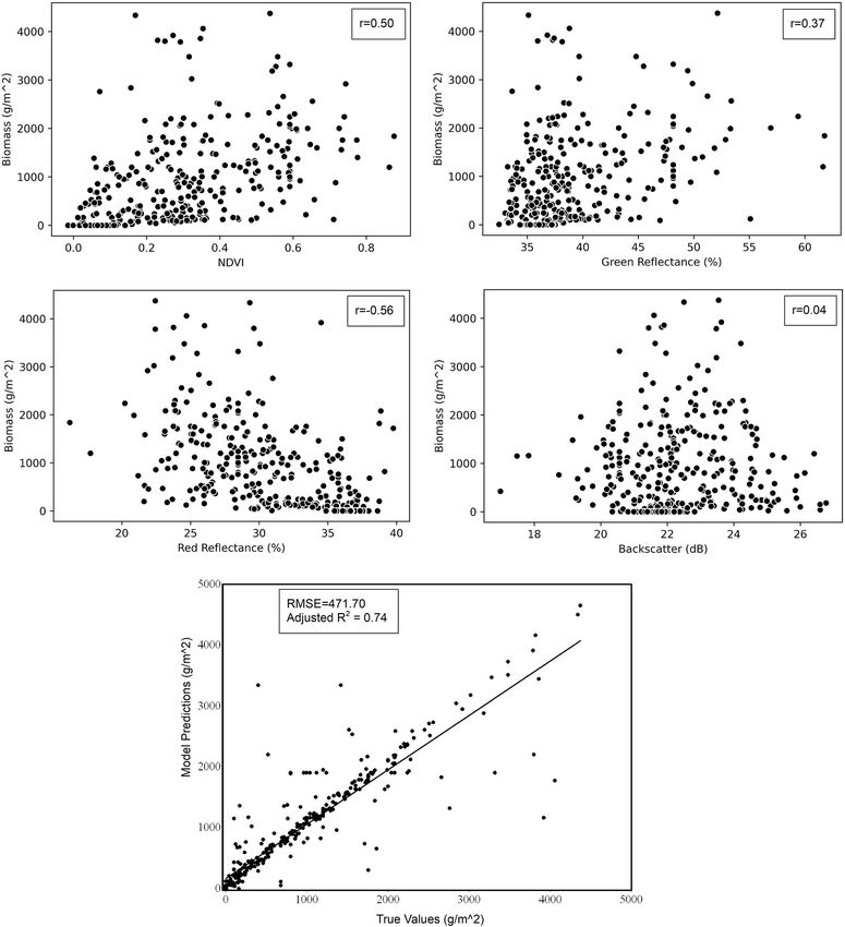
Karki et al.                                                                                                                      Earth Observation for Mapping Blooms

blooms occurs during the summer (Jeffrey et al., 1995;                                      June 2016 and August 2017 following a similar methodology,
Bermejo et al., 2019a, 2020). For this reason, the monitoring of                            were exclusively used for ANN training and validation.
the estuaries and the field sampling were concentrated through
late June to early October. The current study focused on blooms                             Earth Observation Mapping of the
from 2010 to 2018, because of the lack of overlap between field                             Spatial Coverage
surveys and Landsat acquisitions prior to that date.                                        The mapping of macroalgal blooms using satellite imagery
   Bloom extension and biomass abundance were obtained from                                 comprises several steps starting from data download to the
the WFD surveys conducted by the EPA to assess the ecological                               generation of the map (Figure 2). The study utilizes the EO data
status of opportunistic algae blooms on the dates shown in                                  sets from the Sentinel-2 and Landsat (5 and 8) missions to acquire
Table 1. The table shows the dates and locations for which                                  the temporal coverage from 2010 to 2018. The Landsat mission
both field spatial coverage and biomass data sets were available                            from the National Aeronautics and Space Administration
and were collected as a part of the WFD monitoring. Since the                               (NASA) has been operational since 1972, although the availability
WFD method primarily focuses on surveying of algal mats that                                of free and open-source data is a more recent practice that started
are mostly attached, spatial coverage and algal biomass were                                in 2008 (Zhu et al., 2019). To get better temporal coverage from
assessed in situ. The outer edges of the algal accumulations were                           2010, data sets from Landsat-5 Thematic Mapper (TM; data
mapped at low tide using a mapping grade Global Positioning                                 availability:1984–2012) and Landsat-8 Operational Land Imager
System (GPS) unit with accuracy of a meter. A light hovercraft                              (OLI; data availability: 2013–2018) were used. The data sets
was used in areas where the sediment was too soft to allow                                  are freely available from the United States Geological Survey
safe access or where the algal beds were too large to allow safe                            (USGS)’s Earth Explorer2 .
mapping during a single tidal cycle (Wilkes et al., 2017). A series                             Both, Landsat-5 and Landsat-8 missions provide the images
of transects were taken through each patch and haphazardly                                  with a swath width of 185 km and a temporal resolution
distributed 0.5 m2 quadrants were taken along each transect,                                of 16 days (USGS, 2020). These missions are identical from
and their GPS locations were recorded. The percentage cover                                 the application and data processing point of view, especially
and algal biomass in each quadrant were recorded. Biomass                                   for the bands being considered for this study. Landsat bands
from each quadrant was collected, washed, and rinsed in fresh                               in the visible region (red, green, and blue) and NIR are
seawater to remove sand and debris, squeezed dry, and the weight                            available at 30 × 30 m resolution. Unlike Landsat missions,
recorded as g/m2 wet weight. The data were compiled into five                               Sentinel-2 Multispectral Instrument (MSI), under European
sub-metrics (i.e., total percentage cover, total patch size as a                            Space Agency (ESA)’s Copernicus Program, is the newest EO
percentage of available intertidal habitat, average biomass on the                          mission and provides the acquisitions since 2015. It consists of the
intertidal area, average biomass in affected area, and percentage                           constellation of Sentinel-2A and 2B MSI sensors with a combined
of quadrants with algae entrained into sediments) to provide a                              revisit time of 5 days at the equator and swath coverage of 290 km
WFD assessment for the estuaries (Scanlan et al., 2007; Wan et al.,                         (ESA, 2019). The bands required for natural color (red, green,
2017). To meet the requirement for sufficient training data for                             and blue) imagery and vegetation mapping (red and NIR) are
model development, additional data collected as a part of the Sea-                          available at 10 × 10 m resolution. These data sets are available
MAT Project (Bermejo et al., 2019b), not shown in Table 1, were                             freely from ESA’s Sentinel Hub3 .
used. This biomass abundance (g/m2 ) data, collected between
                                                                                            Data Acquisition
                                                                                            The identification of the dates was based on the availability of
                                                                                            the field survey data collected from 2010 to 2018 as a part of
TABLE 1 | Dates of the field investigation and corresponding source of EO data
sets: Landsat-5 TM (L5), Landsat-8 OLI (L8), or Sentinel-2 MSI (S2) missions.               the WFD monitoring program. In response to the number of
                                                                                            field data accompanied by the need to find matching EO scenes
     2010      2013        2014        2015         2016        2017        2018
                                                                                            with low tide and cloud-free conditions, images acquired either
1.                         17-Sep      16 Sept                  10-Jul    21-Sep            before or after the field surveys were indiscriminately considered
                           L8:4-Oct    L8: 5-Sep                S2:17-Jul S2:5-Sep
2.                         19-Sep      15-Sep                   11-Jul    21-Sep
                                                                                            for the study. This is considered the accepted practice in the
                           L8:4-Oct    L8: 5-Sep                S2:17-Jul S2:5-Sep          field of remote sensing and is unlikely to affect the outcome
3. 5-Jul                   18-Sep                               11-Jul                      of the study for mapping Ulva blooms. For each location, the
   L5:19-Jun               L8:4-Oct                             S2:17-Jul                   archival Sentinel-2 data were screened for cloud-free scenes
4.                                                                          27-Sep
                                                                            S2:10-Oct
                                                                                            within two and half weeks of the field monitoring program under
5.                         2-Oct                                            27-Sep
                                                                                            conditions of low tide. In the absence of Sentinel-2 MSI scenes
                           L8:11-Oct                                        S2:10-Oct       (10 m resolution, 2015–2018), Landsat-8 OLI (30 m resolution,
6.                                                  7-Jul                   26-Sep          2013–2018) scenes were used. For scenes prior to 2013 (2010–
                                                    L8:19-Jul               S2:10-Oct
                                                                                            2012), Landsat-5 TM (30 m resolution; 1984–2012) images were
7.             25-Jun      15-Jul                   6-Jul                   12-Jul
               L8:11-Jul   L8:12-Jun                S2:18-Jul               S2:25-Jun       used. Table 1 provides the detailed information about the field
8.                                                  5-Jul                   11-Jul          survey and corresponding source of EO data sets for each of
                                                    S2:18-Jul               S2:28-Jun
                                                                                            2
The dates of field survey are italicized, and the serial number on the left column              https://earthexplorer.usgs.gov/
                                                                                            3
corresponds to the locations shown in Figure 1.                                                 https://scihub.copernicus.eu/

Frontiers in Marine Science | www.frontiersin.org                                       6                                          April 2021 | Volume 8 | Article 633128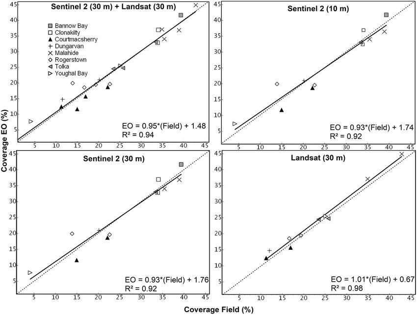
Karki et al.                                                                                                                     Earth Observation for Mapping Blooms

  FIGURE 2 | The workflow developed for mapping blooms using the NDVI delineation technique.

the eight locations. Considering the small number of historical                   NDVI Calculation
WFD monitoring data with associated geospatial information                        Although several remote sensing indices are in use for
followed by the difficulty in finding corresponding EO scenes,                    vegetation mapping, NDVI is the most widely used index
data from 2010 were selected despite the fact that there were no                  (Xue and Su, 2017). The method used in this study is based on
matching scenes for the two subsequent years (2011 and 2012).                     the NDVI for mapping and delineating the bloom. It utilizes
Additionally, 2010 is the only year for which Landsat-5 data                      the characteristic increased reflectance in the NIR region and
were used, which is identical to Landsat-8 from the application                   decreased reflectance in the red regions of the electromagnetic
point of view. Thus, the inclusion of 2010 despite a gap of two                   spectrum exhibited by the vegetation (Jensen, 1986; Tucker and
years and the usage of Landsat-5 was important for this study.                    Sellers, 1986). The NDVI is calculated using Eq. 1.
Sentinel-2 Level 2A (atmospheric corrected) products covering
the areas under consideration were identified and downloaded                                                              (NIR − Red)
                                                                                                              NDVI =                                                (1)
from ESA’s Sentinel Hub website. Similarly, Level 2 Landsat-5 TM                                                          (NIR + Red)
and Landsat-8 OLI products were downloaded from the USGS                             The next step was to compute NDVI using red and NIR bands
Earth Explorer’s website.                                                         in SNAP software. During the band specification, corresponding
                                                                                  bands were identified for Sentinel-2, Landsat-8, and Landsat-5.
                                                                                  All the processing after this step was done using ArcGIS software
Pre-processing
                                                                                  and Python 2.7. Since NDVI computation involves the uses of
The second step involved pre-processing of the scene in order
                                                                                  NIR band, it can overestimate the bloom coverage by including
to reduce the size of the files to allow quick processing in freely
                                                                                  microphytobenthos present in the sediment that contributes to
available Sentinel Application Platform (SNAP) software from
                                                                                  the primary production in an estuarine environment (Launeau
ESA. In the case of Sentinel-2, pre-processing was accomplished
                                                                                  et al., 2018). To prevent this risk, the results from NDVI
as a first step to resize the entire image to the resolution of
                                                                                  needed to be verified with field data. One important advantage
10 m bands (either blue, green, red, or NIR). This step helped to
                                                                                  of using NDVI was its ability to detect live vegetation, due
synchronize all the coarser bands (20 and 60 m) to a resolution
                                                                                  to the consideration of NIR reflectance exhibited only by
of 10 m. This is the most essential step before doing spatial
                                                                                  photosynthetically active plants.
and spectral sub-setting since it helps to significantly reduce the
computing time. After resampling, each scene was resized and                      Generation of Algal Bloom Map
clipped to the extent of each location under investigation. During                The Corine (Coordination of Information on the Environment)
the same step, the spectral sub-setting was completed to retain                   land cover data set4 was used to define area of interest (AOI,
the specific bands required for further processing (blue, green,                  i.e., intertidal mudflats) for each location. Following Corine
red, and NIR). In the case of Landsat-5 and Landsat-8, the scene                  land cover classification, the classes of interest corresponded
was resampled to the extent of 30 m band prior to spatial and
spectral sub-setting.                                                             4
                                                                                      https://www.epa.ie/pubs/data/corinedata/

Frontiers in Marine Science | www.frontiersin.org                             7                                                   April 2021 | Volume 8 | Article 633128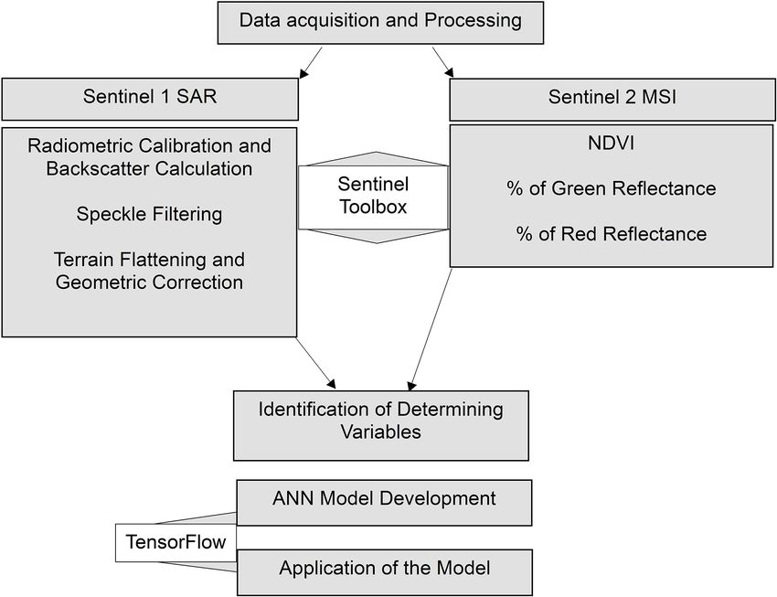
Karki et al.                                                                                                 Earth Observation for Mapping Blooms

with the tidal flats (4.2.3) and estuaries (5.2.2) labels. This               The time gap between the EO data acquisition and field
facilitated the removal of terrestrial vegetation and saltmarshes          survey varied from same day to a maximum of 18 days
from the consideration.                                                    (+/−) with an average of 12 days for 22 pairs of observations.
   The visual inspection was done to determine the threshold               Out of those 22 observations, 12 were Sentinel-2 and 10
of the NDVI values that corresponded with the bloom-forming                were Landsat acquisitions, as we primarily focused on finding
seaweed in the natural color composite. In most cases, NDVI                Sentinel scenes and selected Landsat only when the former
values greater than 0.15 and 0.20 for Sentinel-2 and Landsat               was not available. Since it was not possible to obtain both
images, respectively, represented Ulva blooms. For each location,          Sentinel and Landsat scenes for each location for the same date
the vegetation pixels were segregated after determining the                during the scene selection, more direct comparison between
threshold. This technique was able to segregate bloom patches              the influences of resolutions on identical conditions was not
bigger than a few meters.                                                  possible. To address this, the Sentinel bands were resampled
   Manual verification, subjective judgment, and refinements               to 30 m in order to compare the findings from the 10 m
are essential steps of the mapping workflow to assure that the             Sentinel-2 bands. This helped to compare the overall effects of
bloom pixels are represented correctly. Spatial delineation of the         resolution on the estimated coverage at the same location with
macroalgal blooms using the NDVI technique was the initial                 fine and coarse pixels on the same day. Further, the upscaling
step, and subsequently the computation of biomass relied on the            of the Sentinel bands to 30 m facilitated the comparison with
spatial extent outlined. Correct spatial delineation ensured that          original Landsat bands.
healthy Ulva tissue, as opposed to decomposing tissue, was only
considered. In specific locations, it was necessary to eliminate           Computation of Algal Biomass Using
areas which corresponded to terrestrial vegetation. Due to the             Machine Learning
coarse resolution of Corine land cover data sets, a few areas also         Building upon the spatial coverage extracted using the NDVI
included artificial structures and salt marshes. The minimum               delineation approach, an ANN model was developed to quantify
mapping area for Corine land cover data sets is 50,000 m2 for land         the biomass distribution in the estuarine area. Sentinel-1
cover change and 100 m for linear units. For features smaller than         Synthetic Aperture Radar (SAR) and Sentinel-2 MSI were used
these minimum mapping units, a generalized class is reported in            to develop the ANN model. The in situ biomass samples (point
the Corine database. Because of such boundary generalizations              locations in g/m2 ) collected as a part of WFD monitoring
for small features, these areas were carefully clipped out from            program and those obtained under Sea-MAT project (Bermejo
the AOI polygons. The final step involved the generation of the            et al., 2019b) were compiled as a response variable for the
vector and raster outline of the algal blooms for all locations. The       model. The entire biomass computation process can be broken
area of the bloom was computed, and the percentage coverage                down into data acquisition and processing, identification of
was calculated by taking into account the AOI of each site under           determining variables, model development, and application, as
consideration using the following Eq. 2.                                   shown in Figure 3.

                                                                           Data Acquisition and Processing
    Percentage Cover                                                       Sentinel-2 scenes acquired for mapping spatial coverage of
                                                                           Ulva blooms were also used for biomass calculation. In
        Area delineated by NDVI technique in the AOI                       addition to NDVI, two more products, percentages of green
    =                                                × 100 (2)
                            AOI                                            and red reflectance, were calculated using visible and NIR
                                                                           bands. Altogether 11 Sentinel-2 scenes corresponding to biomass
Validation and Statistical Analysis                                        surveys were used for computing optical variables. Apart from
To test the comparability and consistency of macroalgal blooms             optical data, Sentinel-1 SAR scenes, acquired from ESA’s site,
mapping using satellite imagery and field surveys, and to                  provide the radar information in C-band at a spatial resolution
identify possible disagreement between methodologies, Pearson              of around 10 m. Sentinel-1 images were acquired in either
correlation analyses and paired t-tests (Xu M. et al., 2017) and           ascending or descending modes covering the study area. The
Cohen’s kappa analyses were conducted. The limited number                  standard radar data processing chain (Small and Schubert,
of samples for Landsat show marginal significance compared to              2008; Small, 2011; Filipponi, 2019; Veci, 2019) were followed
other groups, whereas Sentinel with native bands shows higher              using ESA’s Sentinel Toolbox. The processing steps include:(i)
significance. Similarly, the root-mean-square error (RMSE) was             radiometric calibration and calculation of radar backscatter;
calculated to examine the error where lower value indicated                (ii) speckle filtering; and (iii) terrain flattening and geometric
better estimates. Similarly, to assess the influence of the temporal       correction. The final product of the processing was radar
gaps between field surveys and satellite images, the correlation           backscatter in decibels (Raney et al., 1994). Sentinel-1 SAR is
between relative mismatches and the time lapse between                     dual polarized, capable of HH/HV and VH/VV acquisition, but
samplings was evaluated. All statistical analyses were performed           VH/VV is the default mode. Polarization can impact on the
using Minitab software, ArcGIS, and Python packages. When                  results, and cross-polarized (VH) data were found to provide
necessary Shapiro–Wilks and Levene’s tests were used to ensure             better results. Altogether 16 radar scenes corresponding to the
compliance with normality and homoscedasticity assumptions.                biomass field survey data were processed which were acquired
In all statistical analysis, significance was set at 5% risk error.        within 5 days of the data collection. In addition to satellite

Frontiers in Marine Science | www.frontiersin.org                      8                                      April 2021 | Volume 8 | Article 633128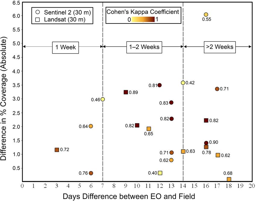
Karki et al.                                                                                                 Earth Observation for Mapping Blooms

  FIGURE 3 | The workflow developed for computing biomass using ANN.

derived variables at the resolution of around 10 m, biomass                neurons and transmit information through structured layers
data collected at the field resolution of 0.5 via field survey were        (Dayhoff and DeLeo, 2001). These interconnected neurons
used in the study.                                                         work exactly like the neurons present in the nervous system
                                                                           of organisms where it learns the relationship among input
Identification of Determining Variables                                    variables through multiple iterations or epochs (Zurada, 1992;
The independent variables were identified, which would explain             Agatonovic-Kustrin and Beresford, 2000; Hu et al., 2018). An
the variability of biomass in the study area. At first, all                ANN consists of different combinations of input variables with
the potential variables that could be related to biomass                   associated empirical weights and bias terms (Huang, 2009).
were considered. Among such variables, NDVI, percentage                    Backpropagation is one of the techniques where parameters
reflectance in green, red, and infrared wavelengths were selected          such as the number of inputs, bias terms, and weights are
as determining variables. Similarly, radar backscatter was                 adjusted in forward and backward fashion until the minimum
considered as one of the determining variables since it is the             error is achieved (Rumelhart et al., 1986; Aggarwal, 2018; Hu
measure of surface roughness. The test of significance and                 et al., 2018). The model training and, hence hyperparameter
redundancy was carried out using variance inflation factor (VIF)           tuning, is attained in several iterations until a stable solution
analysis (O’Brien, 2007) through correlation before selecting the          is achieved. With each iteration of the ANN model, these
independent variables, and only four variables were shortlisted            configurations are tuned so that the structured layers of neurons
for inclusion in the model training because these were found               can model the expected output (Bardenet et al., 2013). During
significant as well as non-redundant. Inclusion of these additional        the ANN development, a small number of validation data
variables for their non-linear contribution is expected to prevent         sets are set aside to prevent overfitting (Shahin et al., 2005;
the potential saturation of NDVI at higher biomass values (Huete           Piotrowski and Napiorkowski, 2013). This step assures that
et al., 2002; Garroutte et al., 2016; Xiao et al., 2017).                  the model is generalized enough, and its robustness does not
                                                                           degrade outside of the training samples. Thus, during the
Development of the Model                                                   model training, the samples should be representative so that the
An ANN models the relationship between the dependent and                   neurons can learn to model the complex relationships adequately
independent variables with the help of training and validation             and appropriately.
data. The model consists of multiple inputs, activation functions,            The ANN model was developed using the total of 346 biomass
hidden layers, and an output which are connected via artificial            samples where the magnitude of biomass (g/m2 ) was the response

Frontiers in Marine Science | www.frontiersin.org                      9                                      April 2021 | Volume 8 | Article 633128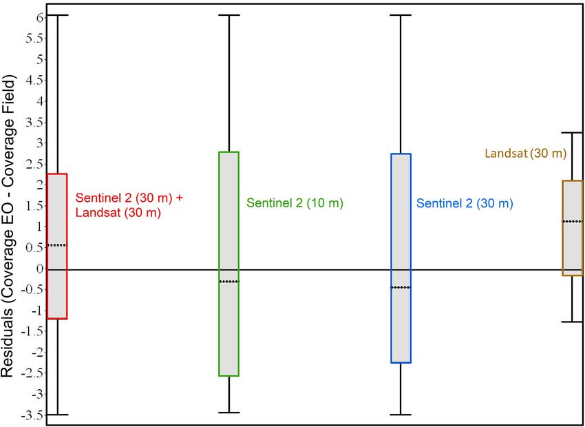
Karki et al. Earth Observation for Mapping Blooms
variable, and remaining variables (NDVI, percentage of green RESULTS
reflectance, percentage of red reflectance, and radar backscatter)
were used as determining variables. Out of the total samples, Spatial Coverage of the Bloom
20% of the data points were used as validation data, where these The extension of the macroalgal blooms from field surveys
prevent the model from overfitting due to excessive training. The ranged between 213,100 and 5,425,900 m2 for Lower Blackwater
hyperparameters, such as the number of hidden layers and the Estuary (2017) and Tolka (2017), respectively. There was a total
number of iterations to achieve a stable solution, were determined of 22 EO estimates with corresponding field survey data, some of
based on the error statistics reported by the model by using which are shown in Figure 4. A significant correlation between
backpropagation-based learning algorithms (Huang, 2009). The EO estimate and survey measurements was observed, which was
fully trained ANN model was achieved with five hidden neurons independent of the satellite missions used (p-values < 0.01).
when the number of epochs reached 50. The learning process All the correlation analyses yielded coefficients of determination
was continued until the model performance plateaued where the close to 1 (between 0.93 and 0.98) and a good fit between the
error was minimal for both validation (20%) as well as training observations (Figure 5). The spatial coverages from EO show
(80%) data sets. The entire process was accomplished using more detailed delineation than those mapped on the ground since
Google’s TensorFlow (Abadi et al., 2016), a free and open-source the field campaign was more concentrated on the predominant
application using Python programming language. The input data and accessible regions of the Ulva blooms. The scatter plots for
preparation was done using ArcGIS, where a table consisting of all the observations made for eight estuaries using Sentinel-2 and
all input variables was generated. Landsat are presented in Figure 5 together with R2 value, slope,
and intercept for each plot.
Although resampled Sentinel-2 bands, upscaled to 30 m, are
Application of the Model a derivative of bands acquired originally at 10 m resolution, it
After the development of the model, the ANN model was applied provided a similar level of performance in terms of delineation
to generate the biomass values using the input variables. In of the green algal blooms and one-to-one correspondence with
order to apply the model, the input data sets were extracted and the field data. The EO data sets show a slight overestimation
compiled in the form of a table. The TensorFlow generated results compared with the field data, as shown in Figure 5. This
were later converted to geographic information system (GIS) overestimation is slightly higher in Figures 5B,C which
raster for mapping and further analysis. The biomass quantity corresponds to Sentinel-2 original and resampled products,
can be predicted for any area as long as input data sets are respectively. For each scatter plot, the equation of the trend
available for any area. line shows the magnitude of the bias, and the slope of the
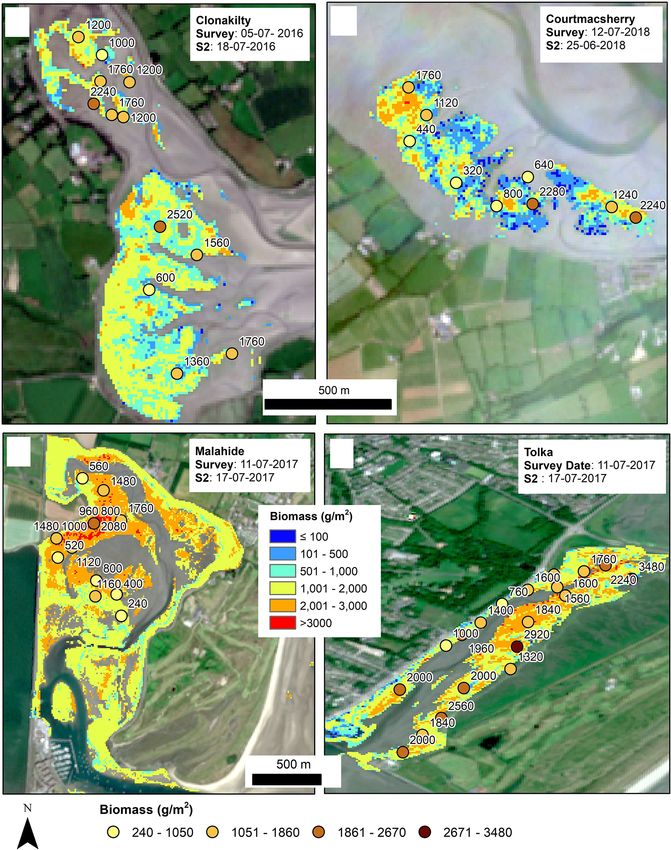
FIGURE 4 | Eight locations showing selected sites with coverages from EO and the corresponding field surveys. Scale bar shows 1 km in all the locations.
Frontiers in Marine Science | www.frontiersin.org 10 April 2021 | Volume 8 | Article 633128Karki et al. Earth Observation for Mapping Blooms
FIGURE 5 | Scatterplots showing the comparison between coverage computed using the EO and coverage obtained using the field survey for four groups based on
the resolutions of the EO data sets: (A) resampled Sentinel-2 30 m and Landsat 30 m, (B) Sentinel-2 10 m, (C) resampled Sentinel-2 30 m, and (D) Landsat 30 m.
The equation of the trend line, the associated R2 values have been shown for each plot. The 45◦ line with 1:1 correspondence between EO and field data has been
shown as a dotted line for reference.
trend line shows the level of estimation (over or under) of observations for Landsat may not statistically prove that
between EO and field survey. Comparing the rate of over- it is performing better than the Sentinel. Overall, the results
and underestimation, Landsat seems to be consistent, although show that native Sentinel-2 bands perform better than resampled
exhibiting a slight overestimation as indicated by the upward bands, as evidenced by lower RMSE. In addition, the resampled
shift of the trend line compared to the 1:1 dotted line. Sentinel-2, Sentinel-2 still managed to provide better results and did not offer
in contrast, shows overestimation for lower magnitudes and a significantly higher error than the native bands.
slight underestimation for higher magnitudes of coverage. These The error analysis was done by comparing the distribution of
under- and overestimations of Sentinel-2 and Landsat imagery the residuals computed between the EO estimates and the field
seem to be compensating each other on the combined scatter plot survey data. After these inter-comparisons of the residuals, it
in Figure 5A. The slope of the regression lines (Figure 5) was is equally important to see if there was any notable correlation
close to 1 for all correlation analyses, and the results of the paired between the difference/discrepancies in percent coverage (EO
t-test (Figure 6 and Table 2) suggest no methodological bias. The estimates and field measurements) with the corresponding time
p-value for all groups of observations shows values higher than lag between them. Thus, the relationship between the differences
0.05, as shown in Table 2. Overall, there was no bias as can be in percent coverage was analyzed against the time lags. Figure 6
seen from Figure 5 and suggested by the paired t-test. shows the differences in bloom coverage estimated using EO and
Regarding the error statistics, the result of the t-test shows field surveys. From the magnitude of the residuals, it is evident
that the RMSE is lowest for Landsat, followed by the RMSE that the differences cannot be considered different to zero in all
for the combination of resampled Sentinel-2 and native Landsat the cases except marginal difference in the case of Landsat. With
bands at 30 m. The Pearson correlation showed the correlation very few observations for less than 1 week and more than 2 weeks,
between EO estimates and field measurements, where Landsat it was difficult to draw any conclusion about the magnitude of the
shows the best results followed by the combination of Sentinel- effect due to the time gap. Figure 7 shows the number of days
2 and Landsat observations. Based on the RMSE and Pearson between those observations and the absolute difference between
correlation values, the Landsat appears to have performed better the percentage coverages. The individual breakdown of Cohen’s
than Sentinel with finer resolution. Nevertheless, the low number kappa for each Sentinel-2 and Landsat observation is indicated
Frontiers in Marine Science | www.frontiersin.org 11 April 2021 | Volume 8 | Article 633128Karki et al. Earth Observation for Mapping Blooms
FIGURE 6 | The box plots showing the residuals computed between the EO estimates and field coverages. The upper and lower bounds of the box represent the
first and third quartiles, whereas the dotted line represents the median. The long horizontal line shows the zero value. The whisker shows the range of the residual
data.
TABLE 2 | Results of the two-sample paired t-test for EO estimates and field the biomass in g/m2 . Only the non-redundant and significant
measurements.
variables were used in the ANN model development based on the
Number of RMSE P-value (paired, two Pearson result from the redundancy test using VIF (O’Brien, 2007) and
Samples value sample for means) correlation correlation analysis. Figure 8 shows the scatter plots of biomass
Sentinel-2 (30) 22 0.71 0.35 0.97
with each of the determining variables where the correlation with
+Landsat (30) red reflectance was highest, followed by NDVI, green reflectance,
Sentinel-2 (10 m) 12 0.93 0.99 0.96 and the radar backscatter. The predicted result was compared
Sentinel-2 (30 m) 12 0.96 0.92 0.96 with the biomass data measured from the field survey with RMSE
Landsat (30 m) 10 0.36 0.06 0.99 value of 471.70 and adjusted R2 of 0.74, as shown in Figure 8E.
The ANN model was used to compute the biomass images for
several estuarine areas. The biomass image shows the distribution
by its label and color code. This figure aids visualization of the of biomass blooms within the areas delineated by the spatial
distribution of data in relation to Cohen’s kappa which highlights coverage mapping technique based on NDVI. Figure 9 shows
the measure of agreement between field and EO estimations. the biomass distribution where both the EO scenes acquisition
Cohen’s kappa value also provides important information about and the field survey were conducted in the summer of 2016
changes in the position of the bloom or the degree of spatial and 2018 for Clonakilty (Figure 9A) and Courtmacsherry
agreement between EO and field data. Most of the observations (Figure 9B), respectively. Similarly, the computed biomasses
clustered around 10–13 days without showing any trend with for Malahide and Tolka for the summer of 2017 are shown in
the difference in the percentage coverage or Cohen’s kappa Figures 9C,D, respectively.
(Figure 7), and the Pearson correlation coefficient indicated no
correlation (Pearson’s r < 0.01) between them.
DISCUSSION
Biomass Computation of the Algal
Blooms Spatial Coverage of the Bloom
The ANN model was developed by using NDVI, percentages The current study used the visible and NIR bands from the
of green and red reflectance, and radar backscatter to compute optical sensors and used the NDVI delineation technique along
Frontiers in Marine Science | www.frontiersin.org 12 April 2021 | Volume 8 | Article 633128Karki et al. Earth Observation for Mapping Blooms FIGURE 7 | The scatter plot for the time gap between EO and field surveys versus the difference in percentage coverage. The number next to each observation and the intensity of color represent Cohen’s kappa coefficient and its magnitude. the tidal flats. Overall, the NDVI technique showed a fine-scale quantities of seaweed biomass because of wind and tidal delineation of blooms than those measured in the field. The currents (Gower et al., 2008; Qiao et al., 2009; Cui et al., reason for a generally better delineation for the EO estimation 2012) has not been considered in this study because algal mats could be due to its sensitivity to even small algal patches producing blooms in Irish estuaries are mostly attached to including microphytobenthos present in the sediment (Launeau the substrate. Additionally, variation in NDVI can arise from et al., 2018). It seems more evident on Sentinel-2 than Landsat, the different stages of macroalgal blooms such as healthy and most likely because of its higher spatial resolution. In contrast, photosynthetically active versus decomposing macroalgal tissue the field survey is generally restricted to the main areas of that can give rise to slightly different measures of NDVI leading the intertidal environment that can be accessed, as shown in to small variations in the spatial coverage. The NDVI-based Figure 4. Considering the increasing average monthly rainfall technique eliminates the need to filter out dead or decomposed in Ireland (80–130 mm; Walsh, 2012) and associated cloud vegetation mapped in contrast to other indices that rely entirely coverage, it is difficult to limit the temporal gaps to a couple of on the spectral reflectance on the visible part of the spectrum days or exclusively select scenes either before or after the field such as red, green, or blue regions. Due to the seasonal surveys. Despite this, a good correlation was obtained followed growth of the macroalgae, the rate of photosynthesis varies by a negligible bias and a slope close to one between satellite with time, thus the use of NDVI can correctly account for the estimates and field survey results, as during the peak bloom corresponding variation in electromagnetic signals indicative of phase (from June to September), the bloom extension might vegetation health (Erener, 2011; Turvey and Mclaurin, 2012). remain more or less constant (relative standard deviation 13– This is particularly important in our case because macroalgal 18%; Monagail et al., 2021, unpublished data). blooms may consist of algae at various states of life cycle Despite these satisfactory results, there may be small variations such as mature algal tissue or actively decomposing mass. in the estimates due to the growth of the bloom during the Furthermore, minor discrepancies may have resulted from time between the satellite overpass and the field surveys. This the methodologies currently being adopted during the field may explain relatively lower Cohen’s Kappa in few locations measurements including human error and sampling bias. These (around 0.4, Figure 7). Similarly, the movement of the large issues were unavoidable considering environmental constraints Frontiers in Marine Science | www.frontiersin.org 13 April 2021 | Volume 8 | Article 633128
Karki et al.                                                                                                                   Earth Observation for Mapping Blooms

  FIGURE 8 | Scatterplots showing the correlation between biomass data from field surveys and other determining variables: (A) NDVI, (B) green reflectance, (C) red
  reflectance, and (D) radar backscatter. Scatterplot on the bottom (E) shows the field survey biomass data versus the predicted biomass from the ANN model.

such as high-cloud coverage, high-tide conditions, and field                          of 0.69 ± 0.13 suggesting a good agreement between field and
limitations such as field safety and accessibility. Planning of                       EO observation.
the field surveys around the satellite overpass can help avoid                           The above observations provide evidence that the mapping
inconsistencies due to daily changes in coverages (Carl et al.,                       results from 10 and 30 m resolutions did not differ significantly
2014). Additionally, there could be some unavoidable errors in                        at the current scale of monitoring of algal blooms. This
the estimation due to the signal mixing that occurs when blooms                       finding is especially helpful in an Irish context, where the
are present along a pixel boundary. Regardless of the sources                         number of scenes is particularly limited by the cloud cover
of error, our data showed an excellent fit when assessing bloom                       as well as low-tide conditions. For areas with optimal weather
coverage with very high R2 (0.94) value with average Kappa value                      conditions, it offers the additional advantage of more frequent

Frontiers in Marine Science | www.frontiersin.org                                14                                              April 2021 | Volume 8 | Article 633128
You can also read