Historical CO2 emissions from land use and land cover change and their uncertainty - Biogeosciences
←
→
Page content transcription
If your browser does not render page correctly, please read the page content below
Biogeosciences, 17, 4075–4101, 2020
https://doi.org/10.5194/bg-17-4075-2020
© Author(s) 2020. This work is distributed under
the Creative Commons Attribution 4.0 License.

Historical CO2 emissions from land use and land cover
change and their uncertainty
Thomas Gasser1 , Léa Crepin1,2 , Yann Quilcaille1 , Richard A. Houghton3 , Philippe Ciais4 , and Michael Obersteiner1,5
1 InternationalInstitute for Applied Systems Analysis (IIASA), 2361 Laxenburg, Austria
2 AgroParisTech,  75231 Paris, France
3 Woods Hole Research Center, 02540 Falmouth, Massachusetts, USA
4 Laboratoire des Sciences du Climat et de l’Environnement, LSCE/IPSL, Université Paris-Saclay,

CEA–CNRS–UVSQ, 91191 Gif-sur-Yvette, France
5 Environmental Change Institute, University of Oxford, OX1 3QY Oxford, UK

Correspondence: Thomas Gasser (gasser@iiasa.ac.at)

Received: 31 January 2020 – Discussion started: 10 February 2020
Revised: 26 May 2020 – Accepted: 24 June 2020 – Published: 13 August 2020

Abstract. Emissions from land use and land cover change           ways to strengthen the robustness of future Global Carbon
are a key component of the global carbon cycle. However,          Budget estimates.
models are required to disentangle these emissions from the
land carbon sink, as only the sum of both can be physically
observed. Their assessment within the yearly community-
wide effort known as the “Global Carbon Budget” remains
a major difficulty, because it combines two lines of evidence     1   Introduction
that are inherently inconsistent: bookkeeping models and dy-
namic global vegetation models. Here, we propose a unifying       The annual flux of carbon dioxide (CO2 ) to the atmosphere
approach that relies on a bookkeeping model, which embeds         caused by land use and land cover change (LULCC) is a
processes and parameters calibrated on dynamic global veg-        key part of the Global Carbon Budget (GCB; Friedlingstein
etation models, and the use of an empirical constraint. We        et al., 2019). It is one of the two historical anthropogenic
estimate that the global CO2 emissions from land use and          sources of CO2 (along with fossil fuel burning and indus-
land cover change were 1.36 ± 0.42 PgC yr−1 (1σ range) on         try emissions), and when added to the land carbon sink it
average over the 2009–2018 period and reached a cumula-           gives the net land-to-atmosphere carbon exchange. In fact, it
tive total of 206 ± 57 PgC over the 1750–2018 period. We          is so closely connected to the land carbon sink that choos-
also estimate that land cover change induced a global loss        ing incompatible definitions for these two fluxes can lead to
of additional sink capacity – that is, a foregone carbon re-      double counting or missing part of the budget (Gasser and
moval, not part of the emissions – of 0.68 ± 0.57 PgC yr−1        Ciais, 2013). Thus, models are required to disentangle these
and 32 ± 23 PgC over the same periods, respectively. Addi-        emissions from the land carbon sink, because only the sum of
tionally, we provide a breakdown of our results’ uncertainty,     both can be physically observed. The Global Carbon Budget
including aspects such as the land use and land cover change      2019 (GCB2019) assessment (Friedlingstein et al., 2019) es-
data sets used as input and the model’s biogeochemical pa-        timated that LULCC emissions were 1.5 ± 0.7 PgC yr−1 (1σ
rameters. We find that the biogeochemical uncertainty domi-       range) on average over the 2009–2018 period. This value
nates our global and regional estimates with the exception of     relied on two lines of evidence: dynamic global vegetation
tropical regions in which the input data dominates. Our anal-     models (DGVMs), which are complex process-based and
ysis further identifies key sources of uncertainty and suggests   spatially explicit models of the terrestrial carbon cycle (and
                                                                  related processes), and bookkeeping models, which are para-
                                                                  metric models that convolute time series of LULCC areal

Published by Copernicus Publications on behalf of the European Geosciences Union.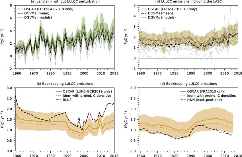
4076                                                  T. Gasser et al.: Historical CO2 emissions from land use and land cover

perturbations with empirical response functions describing           process-based) models at the yearly timescale (although it
changes in ecosystem carbon stocks after these perturbations.        cannot generate inter-annual variability by itself). Its land
   The strengths and weaknesses of those two types of mod-           carbon cycle is calibrated on DGVMs; it is not spatially re-
els are contrasting: DGVMs are developed to precisely de-            solved, but it is subdivided into 10 broad world regions and
scribe the biogeochemistry of plants and ecosystems, albeit          5 biomes (see Appendix A1 for a more detailed descrip-
without overly focusing on LULCC, whereas bookkeeping                tion). The model’s preindustrial steady state is calibrated on
models are specifically designed to evaluate LULCC emis-             the exact same simulations made for the GCB (also called
sions, although without any explicit representation of biogeo-       the TRENDY exercise), and it does not require any spin-up.
chemical processes. Any comparison between those mod-                The transient responses of net primary productivity, wild-
els is rendered even more difficult by two factors. First,           fires, and heterotrophic respiration to changes in atmospheric
DGVMs and bookkeeping models do not naturally follow                 CO2 and climate are calibrated on Coupled Model Intercom-
the same definition of LULCC emissions, as DGVMs tend                parison Project 5 (CMIP5) simulations (Arora et al., 2013).
to include the “loss of additional sink capacity” (LASC) in          Its bookkeeping module keeps track of ecosystems affected
their estimate (Gasser and Ciais, 2013; Pongratz et al., 2014).      by LULCC separately, offering a consistent and easy way
The LASC is defined as the difference between the actual             to isolate LULCC emissions from the land sink (Gasser and
land sink under changing land cover and the counterfac-              Ciais, 2013; Gasser et al., 2017). The LULCC activities ac-
tual (stronger) land sink under preindustrial land cover. The        counted for are gross land cover change transitions, wood
LASC, however, is not an actual physical flux: it is a foregone      harvest (without land cover change), and shifting cultivation
carbon removal. (A few DGVMs are now capable of provid-              (i.e., rapid rotations between young natural ecosystems and
ing LULCC emissions that are consistent with the bookkeep-           cropland). OSCAR does not include fire as a land manage-
ing definition; however, these estimates are not used to estab-      ment tool (Houghton et al., 2012), the emissions caused by
lish the best-guess estimates for the GCB (Friedlingstein et         the draining and burning of peatlands (Carlson et al., 2015;
al., 2019).) The second source of discrepancy is the differ-         Guillaume et al., 2018; Houghton and Nassikas, 2017), or
ent historical LULCC data sets used to drive the models. In          the impact of LULCC on the export of terrestrial organic
the GCB2019, the DGVMs and one of the two bookkeeping                carbon to the ocean via the land–ocean aquatic continuum
models (Hansis et al., 2015) used spatially explicit LULCC           (Regnier et al., 2013). Here, we use OSCAR v3.1: an iter-
drivers from the “Land-Use Harmonization” (LUH) project              ation over v3.0 in which the land carbon cycle’s structure
(Hurtt et al., 2006, 2011). The second bookkeeping model             was slightly altered and its preindustrial steady state was re-
(Houghton and Nassikas, 2017), however, used independent             calibrated. Both changes are described in Appendix A2, and
driving data compiled from national statistics of the United         older changes that led from v2.2 to v3.0 are summed up in
Nation’s Food and Agriculture Organization (FAO), espe-              Appendix A3. OSCAR v2.2 has been comprehensively de-
cially from its Global Forest Resources Assessment 2015              scribed by Gasser et al. (2017). These and earlier versions
(FRA2015; FAO, 2015).                                                have been used in the past to investigate LULCC emissions
   Here, using the OSCAR reduced-form Earth system                   (Arneth et al., 2017; Bastos et al., 2016; Eglin et al., 2010;
model, we bridge the gap between these approaches and es-            Gasser and Ciais, 2013; Gitz and Ciais, 2003).
timates. OSCAR embeds a bookkeeping module as well as                   We follow an experimental protocol similar to that used
simplified biogeochemical processes calibrated on DGVMs;             in the recent GCBs (and fully described in Appendix A4).
this makes it a valuable tool to consistently bridge across the      The model is driven with observed changes in environmen-
different estimates used in the GCB, as illustrated in Table 1.      tal conditions (global atmospheric CO2 , regional tempera-
Thus, the goal of this paper is threefold: first, it is to provide   ture, and precipitation) and with specific LULCC driving
another bookkeeping estimate of global and regional LULCC            data. Thanks to the model’s flexibility and low computing
emissions – that will hopefully be used in the future GCB –          requirements, we also run different LULCC data sets, sen-
obtained with an original model; second, it is to revise and         sitivity experiments in which either changes in environmen-
further investigate the LASC estimates that we provided in           tal conditions or LULCC are turned off, and a Monte Carlo
an earlier version of the GCB (Le Quéré et al., 2018b); and,         ensemble of 10 000 different biogeochemical parameteriza-
third, it is to investigate the uncertainty range in both these      tions. These parameterizations are drawn randomly and with
fluxes along the three axes of analysis shown in Table 1: the        equiprobability from a pool of potential sets of parameters.
inclusion of the LASC, the driving LULCC data sets, and the          This main pool is obtained by combining smaller pools of
biogeochemical parameterization.                                     available parameterizations for separate processes (or groups
                                                                     of processes), as described by Gasser et al. (2017). For in-
                                                                     stance, recalibration of the preindustrial steady state led to
2   Overview of the methodology                                      11 possible parameterizations for preindustrial net primary
                                                                     productivity and turnover times, 4 for preindustrial wildfire
OSCAR is a reduced-complexity model built to emulate the             rates, 5 for preindustrial export fractions from crop harvest-
behavior of more complex (typically three-dimensional and            ing, and 2 for those from animal grazing. This is already a

Biogeosciences, 17, 4075–4101, 2020                                                    https://doi.org/10.5194/bg-17-4075-2020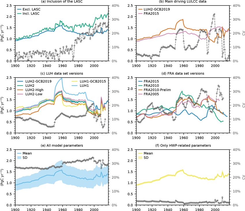
T. Gasser et al.: Historical CO2 emissions from land use and land cover                                                                             4077

Table 1. Availability of LULCC emissions estimates in the GCB2019 and this study. This follows our three main axes of analysis: the
definition of LULCC emissions (i), the driving data sets (ii), and the biogeochemical parameterization (iii).

                                                                GCB2019 (Friedlingstein et al., 2019)             OSCAR (this study)
             (i) Definition (→)                                  Excl. LASC          Incl. LASC              Excl. LASC          Incl. LASC
             (ii) LULCC data set (→)                            LUH     FRA     LUH           FRA           LUH       FRA       LUH       FRA
             (iii) Biogeochemical parametersa (↓)
             BLUE                                                 X
             H&N                                                         X
             CABLE-POP                                                           X                            X         X         X         X
             CLASS-CTEM                                                          X                            X         X         X         X
             CLM5.0b                                                             X
             DLEM                                                                X                            X         X         X         X
             ISAM                                                                X                            X         X         X         X
             JSBACH                                                              X                            X         X         X         X
             JULES                                                               X                            X         X         X         X
             LPJb                                                                X
             LPJ-GUESS                                                           X                            X         X         X         X
             LPX-Bernb                                                           X
             OCN                                                                 X                            X         X         X         X
             ORCHIDEE                                                            X                            X         X         X         X
             ORCHIDEE-CNP                                                        X                            X         X         X         X
             SDGVMb                                                              X
             SURFEXb                                                             X
             VISIT                                                               X                            X         X         X         X
           a BLUE (Hansis et al., 2015) and H&N (Houghton and Nassikas, 2017) are bookkeeping models, whereas the others are DGVMs. b OSCAR could
           not be calibrated on these DGVMs due to insufficient data.

total of 11 × 4 × 5 × 2 = 440 parameterizations. These are                       3     Results and comparison with existing estimates
further combined with available parameterizations for other
elements such as the transient response of the land carbon cy-                   3.1     Global LULCC emissions and LASC
cle to atmospheric CO2 and climate change or the handling
of harvested wood products, which leads to a main pool of                        Our primary results are shown in Table 2 and Fig. 1. We
∼ 1.5 million sets of parameters.                                                find global LULCC emissions of 1.36 ± 0.42 PgC yr−1 on
   Our best-guess estimate is derived by combining the re-                       average over the 2009–2018 period, which is consistent
sults obtained with two LULCC data sets: the latest iteration                    with the GCB2019 estimate (Friedlingstein et al., 2019) of
of the LUH2 data set used for the GCB2019 (Friedlingstein et                     1.5 ± 0.7 PgC yr−1 . Our reported value follows a bookkeep-
al., 2019) and the FRA2015 data set used by Houghton and                         ing definition (Gasser and Ciais, 2013; Pongratz et al., 2014)
Nassikas (2017). However, the latter data set ends in 2015;                      and is therefore comparable to that of the GCB. We sim-
therefore, we extended its results with constant values over                     ulate that historical LULCC emissions peaked at a value
the 2016–2018 period equal to the average of the 2011–2015                       of 1.61 ± 0.55 PgC yr−1 in 1959. Since then, they have re-
period. To constrain this best-guess ensemble, each of the                       mained roughly steady, but they reached a local minimum
20 000 elements is given a weight based on how well it com-                      of 1.14 ± 0.52 PgC yr−1 in 1999. Overall, we estimate that a
pares to a reference value. All results presented in this study                  total of 206 ± 57 PgC was emitted between 1750 and 2018,
are the ensuing weighted averages and weighted standard de-                      and a total of 178 ± 50 PgC was emitted between 1850 and
viations (see Appendix A5). The chosen constraining value                        2018. These values are also consistent with the GCB2019 es-
is the net change in the land carbon stock between 1850 and                      timates of 235 ± 75 and 205 ± 60 PgC over the same periods,
2018, which is estimated to be −25 ± 30 PgC. It is calcu-                        respectively.
lated via the carbon balance over the chosen period using the                       We estimate a global LASC of 0.68 ± 0.57 PgC yr−1 on
GCB2019 estimates of cumulative fossil fuel emissions and                        average over the 2009–2018 period. This amounted to a cu-
changes in atmospheric and oceanic carbon stocks as well as                      mulative total of 32 ± 23 PgC between 1750 and 2018 and
standard uncertainty propagation.                                                to 31 ± 22 PgC between 1850 and 2018. This extremely low
                                                                                 difference between the two periods is explained by the na-
                                                                                 ture of the LASC. It is a foregone land carbon sink – a

https://doi.org/10.5194/bg-17-4075-2020                                                                       Biogeosciences, 17, 4075–4101, 2020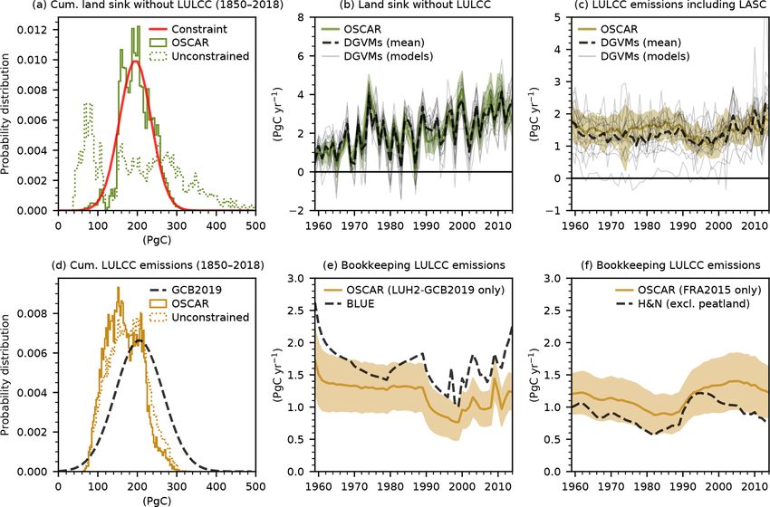
4078                                                   T. Gasser et al.: Historical CO2 emissions from land use and land cover

Figure 1. Our best-guess estimates of bookkeeping LULCC emissions and LASC. Panel (a) shows annual fluxes, and panel (b) shows
cumulative fluxes. The net land-to-atmosphere flux is also shown in panel (b) and compared with the constraint (red). Shaded areas show the
1σ uncertainty range. Panel (c) shows the detailed probability distributions of the cumulative net land flux, land sink, and LULCC emissions
in the unconstrained (dotted histograms) and constrained (plain histograms) output ensemble (20 000 Monte Carlo elements) compared with
the constraint (red) and the GCB estimates (dashed black).

product of both land cover change and environmental condi-                 The effect of the constraint is further detailed in Fig. 1c.
tion changes. Since environmental conditions only changed               Since the constraint is applied to the cumulative net land-
marginally during the early 1750–1850 period, the land sink             to-atmosphere flux over the 1850–2018 period, it corrected
and the LASC were extremely low. As the change in envi-                 the overestimate and substantially reduced the spread of this
ronmental conditions became more intense in the recent past,            value: from an unconstrained −4 ± 84 PgC to −22 ± 29 PgC
both fluxes increased in intensity. Our new estimates of the            (compared with the constraining value of −25±30 PgC). Ap-
LASC are larger than those we reported in a past GCB (Le                plying the constraint essentially resulted in the exclusion of
Quéré et al., 2018b) owing to the change in the empirical con-          aberrant values of the land carbon sink without significantly
straint. Table 2 shows that we indeed obtain estimates similar          affecting LULCC emissions. The cumulative LULCC emis-
to prior estimated values by reverting back to the old con-             sions over the 1850–2018 period were indeed 176 ± 48 PgC
straint (which was the cumulative land sink over the 1850–              before the constraint was applied (and 178 ± 50 PgC after).
2018 period without LULCC simulated by DGVMs). The                      As similar processes drive the LASC and the land sink, the
performance of this alternative constraint is further discussed         stronger constraining effect on the land sink is also logically
later in this paper and is shown in Fig. A1 in the Appendix.            visible on the LASC: the unconstrained cumulative LASC

Biogeosciences, 17, 4075–4101, 2020                                                         https://doi.org/10.5194/bg-17-4075-2020
T. Gasser et al.: Historical CO2 emissions from land use and land cover                                                      4079

over the 1850–2018 period was 25 ± 23 PgC (and the con-           3.3   Uncertainty analysis
strained value was 32 ± 23 PgC).
                                                                  Although we cannot investigate the aforementioned struc-
3.2   Comparison with GCB models                                  tural differences between bookkeeping models, our exper-
                                                                  imental setup allows for the investigation of several fac-
Comparability between our best-guess estimates and those          tors within OSCAR that affect the spread in our global re-
of the GCB2019 is limited (due to the differing definitions or    sults. Figure 3 and Table 3 summarize this. The first fac-
driving data); therefore, we dedicate this section to compar-     tor is whether the LASC is included in the estimate of the
ing like to like. Figure 2a compares the annual land sink over    LULCC emissions, as this is usually the case when they
the 1959–2018 period in the absence of the LULCC perturba-        are calculated with DGVMs, which is illustrated in Fig. 3a.
tion (i.e., with a preindustrial land cover). OSCAR simulates     Over the last decade, the difference between including and
a slightly larger land sink by the end of the period than the     excluding the LASC corresponds to a debiased 1σ range of
DGVMs, although it remains within their uncertainty range.        ±0.43 PgC yr−1 and a coefficient of variation (CV) of ±25 %
It also reproduces the inter-annual variability of the complex    (see Appendix A6). This rather substantial value is in line
models fairly well. Note that this specific simulation is used    with previous studies that quantified this discrepancy (Gasser
by the GCB to define the land sink. This implies that their       and Ciais, 2013; Stocker and Joos, 2015). Because the LASC
land sink is not comparable to ours (except in this figure),      only became non-negligible in the recent past, the effect of
as theirs does not include the LASC. Figure 2b compares           its inclusion or exclusion on cumulative LULCC emissions
LULCC emissions calculated using the DGVMs’ definition            is smaller than for recent annual emissions: we estimate that
(Gasser and Ciais, 2013; Pongratz et al., 2014; i.e., includ-     it is only ±20 PgC (±9 %) over the 1750–2018 period. How-
ing the LASC) over the 1959–2018 period. OSCAR is in line         ever, it is crucial to understand that the intensity of this dis-
with the DGVMs, although it estimates a slightly larger flux      crepancy will keep increasing and accumulating as long as
over the beginning of the period. More importantly, it dis-       changes in environmental conditions do not stabilize (Gasser
plays a much lower uncertainty range than the spread among        and Ciais, 2013). This is illustrated by the positive trend in
DGVMs. Since OSCAR emulates the carbon densities of the           the CV in Fig. 3a. In our view, this ever-growing discrep-
DGVMs well (Table A1 in the Appendix), we attribute this          ancy strongly pleads in favor of choosing, retaining, and con-
difference in spread to the large variance in the land cover      sistently applying one clear definition of LULCC emissions.
map used by the DGVMs (Table A2) and their processing of          In the following, we exclude the LASC from LULCC emis-
the input LULCC data set.                                         sions; therefore, we discuss it separately.
   Figure 2c compares OSCAR and BLUE estimates of the                 The second factor of uncertainty is the driving LULCC
bookkeeping LULCC emissions (i.e., without the LASC).             data set. Figure 3b shows the difference between the average
BLUE is one of the two bookkeeping models used in                 bookkeeping emission estimates based on LUH2-GCB2019
the GCB2019, and both models are driven by the LUH2-              and those based on FRA2015. We find that the annual emis-
GCB2019 data set. OSCAR and BLUE display similar an-              sions from the two data sets are in particularly good agree-
nual variations in their LULCC emissions, but BLUE is sys-        ment on average over the last decade (Table 3), although
tematically higher than OSCAR, and it is above the 1σ range       this is purely fortuitous as the discrepancy is ±0.30 PgC yr−1
of our estimates by the end of the simulation. Figure 2d com-     (±24 %) over the 1995–2004 period and even peaks at
pares OSCAR and H&N estimates (also without the LASC).            ±0.39 PgC yr−1 (±34 %) in 1999. More worrying, perhaps,
H&N is the second bookkeeping model of the GCB2019, and           is the two data sets’ disagreement on the trend in emis-
this time both models are driven by the FRA2015 data set.         sions after 1990. This discrepancy is hidden in our best-
Again, both models display similar annual variations, except      guess emissions that are rather even over the last 30 years. In
near the end of the simulation, and this time H&N is sys-         terms of cumulative emissions over the 1750–2018 period,
tematically lower than OSCAR, although it remains mostly          however, results from the two data sets are in good agree-
within its 1σ range. Given that BLUE and H&N are parame-          ment, with only a ±8 PgC (±4 %) discrepancy. Addition-
terized with the same carbon densities, one would expect that     ally, Fig. 3c and d display the same source of uncertainty but
OSCAR’s estimates would systematically be either higher or        among different versions of each of the two main data sets.
lower. The fact that this is not the case suggests that part of   This variation, which is caused by updating the data sets, is
the differences between the three bookkeeping models pos-         visible, for instance, when comparing older versions of the
sibly stems from other factors such as structural assumptions     GCB with one another. We find that the difference among
or ways of processing and implementing the LULCC data             several versions of the same data set is of the same order of
sets.                                                             magnitude as the difference between our two main data sets.
                                                                  For the LUH data set, this is explained by several factors,
                                                                  from the simple update of the historical land cover data used
                                                                  as input (Klein Goldewijk et al., 2017; Klein Goldewijk et al.,
                                                                  2011) to the complete overhaul of how shifting cultivation is

https://doi.org/10.5194/bg-17-4075-2020                                                  Biogeosciences, 17, 4075–4101, 2020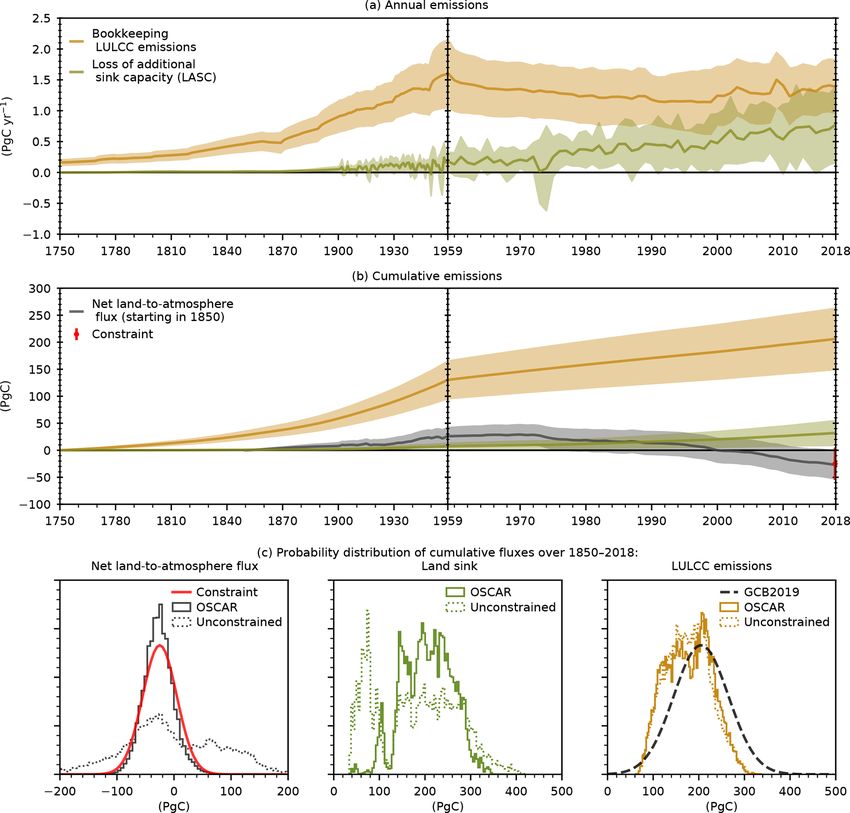
4080                                                            T. Gasser et al.: Historical CO2 emissions from land use and land cover

Table 2. Estimates of the global net land-to-atmosphere flux, LULCC emissions, land sink, and LASC. Estimates following our default (i.e.,
best-guess) and alternative constraints are provided. The land sink includes the LASC; therefore, the net land-to-atmosphere flux is strictly
equal to the LULCC emissions minus the land sink.

                                                                Annual flux (PgC yr−1 )                  Cumulative flux (PgC)
                                                                       2018         2009–2018       1850–2018             1750–2018
                Default constraint (net land flux as residual from fossil emissions, atmospheric growth, and the ocean sink)
                Net land-to-atmosphere flux∗                −1.85 ± 0.75         −1.62 ± 0.79        −27 ± 26              −22 ± 29
                Bookkeeping LULCC emissions                  1.39 ± 0.43          1.36 ± 0.42        178 ± 50              206 ± 57
                Land carbon sink                             3.24 ± 1.02          2.98 ± 1.02        205 ± 53              228 ± 59
                Loss of additional sink capacity             0.78 ± 0.62          0.68 ± 0.57         31 ± 22               32 ± 23
                Alternative constraint (land sink without LULCC perturbation as estimated by the DGVMs)
                Net land-to-atmosphere flux∗                −1.51 ± 0.66         −1.33 ± 0.71        −16 ± 47               −9 ± 54
                Bookkeeping LULCC emissions                  1.27 ± 0.36          1.26 ± 0.36        166 ± 44               192 ± 51
                Land carbon sink                             2.78 ± 0.68          2.58 ± 0.73        181 ± 36               201 ± 40
                Loss of additional sink capacity             0.51 ± 0.33          0.44 ± 0.32         21 ± 11                22 ± 11
              ∗ Counted algebraically: negative values denote carbon removal from the atmosphere.

Figure 2. Comparison of our results with the GCB2019. (a) The annual terrestrial carbon sink in the absence of the LULCC perturbation
simulated by OSCAR (color), the individual GCB DGVMs (light gray), and their multi-model mean (dashed black). (b) The annual LULCC
emissions deduced from the GCB DGVMs (i.e., including the LASC). (c) Bookkeeping LULCC emissions when the model is driven by the
LUH2-GCB2019 data set compared with BLUE estimates reported by the GCB2019. The dotted line shows the same emissions but when
carbon densities are kept at their preindustrial level throughout the simulation (shown without uncertainty for legibility). (d) Bookkeeping
LULCC emissions when the model is driven by the FRA2015 data set compared with the H&N estimates from which emissions from
peatlands were subtracted. All shaded areas show the 1σ uncertainty range. “Idem” stands for “same as above”.

Biogeosciences, 17, 4075–4101, 2020                                                                      https://doi.org/10.5194/bg-17-4075-2020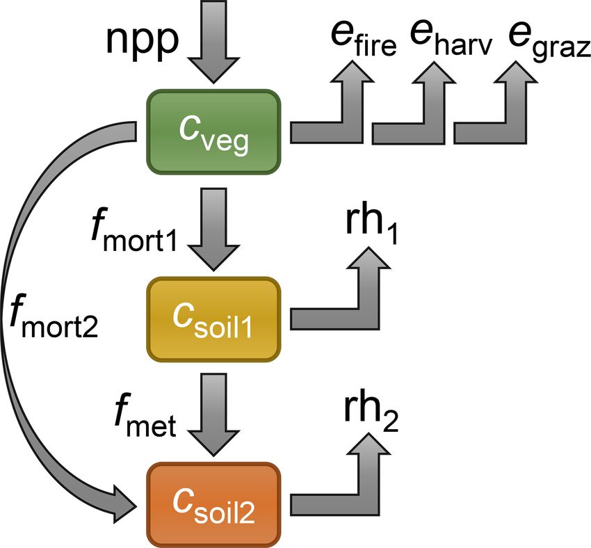
T. Gasser et al.: Historical CO2 emissions from land use and land cover                                                                        4081

Table 3. Uncertainty sources in our estimates of bookkeeping LULCC emissions and LASC expressed as the debiased standard deviation
(1σ ) and the coefficient of variation (CV; in parentheses).

                                                                     Annual flux (PgC yr−1 )               Cumulative flux (PgC)
                                                                    1995–2004             2009–2018      1850–2004         1750–2018
                     Uncertainty breakdown of bookkeeping LULCC emissions
                     (i) Definition                              ±0.31 (21 %)         ±0.43 (25 %)       ±14 (8 %)          ±20 (9 %)
                     (ii) LULCC data set                         ±0.30 (24 %)          ±0.03 (2 %)        ±8 (5 %)           ±8 (4 %)
                     – LUH data set version                      ±0.14 (14 %)                    –       ±14 (8 %)                  –
                     – FRA data set version∗                     ±0.25 (21 %)                    –      ±15 (10 %)                  –
                     (iii) Biogeochemical parameters             ±0.40 (32 %)         ±0.40 (29 %)      ±43 (27 %)         ±55 (27 %)
                     – only HWP-related parameters                ±0.03 (2 %)          ±0.02 (2 %)        ±4 (2 %)           ±5 (3 %)
                     Uncertainty breakdown of the loss of additional sink capacity
                     (ii) LULCC data set                         ±0.14 (28 %)         ±0.21 (31 %)       ±7 (31 %)         ±10 (31 %)
                     (iii) Biogeochemical parameters             ±0.35 (75 %)         ±0.50 (77 %)      ±13 (62 %)         ±19 (63 %)
                   ∗ These values were taken directly from Houghton and Nassikas (2017); therefore, they were not computed with OSCAR. They
                   include some biogeochemical uncertainty, although to a lesser but unknown degree.

estimated (Heinimann et al., 2017). Among the FRA-based                             gests that the latter is kept relatively low thanks to compen-
data set’s versions, this difference is found to be somewhat                        sation effects that do not come into play in the former. We
larger. This is likely due to the concomitant update of some                        also find that the biogeochemical uncertainty in the LASC is
biogeochemical parameters of the H&N model (Houghton                                high: ±0.50 PgC yr−1 (±77 %) for the annual flux over the
and Nassikas, 2017) that we cannot separate here, because                           2009–2018 period and ±19 PgC (±63 %) for the cumulative
the results shown in Fig. 3d are not based on OSCAR.                                flux over the 1750–2018 period. These values reflect the large
    The third and last factor of uncertainty is the parameteri-                     uncertainty in the ecosystems’ response to transiently chang-
zation of the model (for biogeochemistry). Using our Monte                          ing environmental conditions, despite our constraints (uncon-
Carlo ensemble, we find a weighted standard deviation of                            strained CVs are ±98 % and ±86 % for the abovementioned
±0.40 PgC yr−1 (±29 %) for annual emissions averaged over                           time periods, respectively).
the 2009–2018 period and of ±55 PgC (±27 %) for emis-
sions cumulated over the 1750–2018 period. Except in some                           3.4     Breakdown by region
specific years, this source of uncertainty in annual emissions
is the largest of the three we studied, and it dominates without
exception in cumulative emissions. Carbon densities (and the                        Figure 4 and Table 4 provide our best-guess estimates of the
parameters determining them) are the key modeling factors                           bookkeeping LULCC emissions in our 10 broad world re-
explaining this spread (Gasser and Ciais, 2013). Figure 3f                          gions. Unsurprisingly, tropical regions (Latin America, sub-
and Table 3 show the spread in our results when looking only                        Saharan Africa, and South and Southeast Asia, in decreasing
at the variation caused by the parameters that relate to har-                       order) are found to be the main LULCC emitters over the
vest wood products (HWPs). It is found to be one order of                           last decade, with a positive trend over the last 50 years. Con-
magnitude smaller than the total uncertainty caused by all                          versely, North America, Europe, the former Soviet Union,
parameters, confirming that biogeochemical parameters ex-                           and China are all found to have a decreasing trend over the
plain most of the uncertainty. However, we acknowledge that                         last 50 years – to the point of North America, Europe, and
OSCAR likely underestimates the HWP-related uncertainty,                            China being net carbon absorbers over the last decade. Look-
because there is only one option to choose from (in the Monte                       ing at a larger historical period, Latin America and South and
Carlo setup) regarding how HWPs are split between pools                             Southeast Asia were the top two emitters over the 1750–2018
with different decay timescales (Appendix A7).                                      period, with North America being the third-highest emitter.
    Finally, a similar uncertainty breakdown for the LASC is                        It must be noted, however, that this ranking is not statistically
reported in Table 3. We find that the uncertainty in the aver-                      significant due to uncertainties. When the subset of our sim-
age annual LASC between our two main LULCC data sets                                ulations driven by the FRA2015 data set is isolated, our esti-
over the last decade is ±0.21 PgC yr−1 (±31 %), and it is                           mates compare very well to the estimates of H&N (Houghton
±10 PgC (±31 %) for the cumulative LASC since the year                              and Nassikas, 2017; see Table A3 in Appendix).
1750. The much higher CV in the cumulative LASC com-                                   The uncertainty in our regional bookkeeping LULCC
pared with that in the cumulative LULCC emissions sug-                              emissions can be attributed to the LULCC data sets and the
                                                                                    biogeochemical parameters using Fig. 4 and Table 4. For

https://doi.org/10.5194/bg-17-4075-2020                                                                         Biogeosciences, 17, 4075–4101, 2020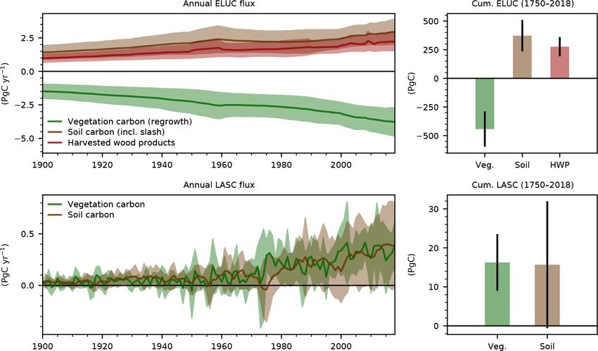
4082                                                     T. Gasser et al.: Historical CO2 emissions from land use and land cover

Figure 3. Variations and uncertainties in the time series of global annual LULCC emissions. (a) The effect of adding the LASC to LULCC
emissions. (b) The effect of the LULCC driving data sets (only the two data sets used to estimate our best guess). (c) The effect of the data set
version among the LUH variants (not used for our best guess). (d) The effect of the data set version among FRA variants. These emissions
were not simulated by OSCAR; they were reported by Houghton and Nassikas (2017; their Fig. 8). (e) The effect of all of the parameters
of OSCAR (using the weighted Monte Carlo ensemble). (f) The effect of the subset of parameters of OSCAR that are related to harvested
wood products (i.e., the parameters that are not derived from DGVMs). All panels show bookkeeping LULCC emissions with the obvious
exception of panel (a). Thick colored lines show the values obtained by averaging over all axes of analysis apart from the one investigated
in the panel. The dashed gray lines with markers show the debiased coefficients of variation (CVs), i.e., the ratios of the debiased standard
deviation over the average, and refer to the y axis on the right-hand side of each panel.

North America, the former Soviet Union, and, to a lesser ex-               nores those declarations and considers that China lost a large
tent, Europe, the two LULCC data sets lead to emissions that               amount of forest over the same period. Ultimately, it is not
are in rather good agreement; this implies that the regional               the goal of this paper to provide a detailed analysis of the re-
uncertainty is dominated by the biogeochemical parameteri-                 gional discrepancies between the two data sets nor to recom-
zation. In tropical regions, however, the two data sets show               mend one over the other. Nevertheless, we produced Fig. A2,
substantial disagreement – to the point of being the main                  which shows regional LULCC drivers, to offer a starting
source of uncertainty in sub-Saharan Africa and in South and               point for such an endeavor.
Southeast Asia. Remarkably, the disagreement in the emis-                     Our estimate of the LASC is also broken down regionally
sions of Latin America is shown in Fig. 4, but the inverse                 in Fig. 4. The annual LASC of most regions follows a sim-
global trends is shown in Fig.3b. China is another region in               ilar trend to the global one. However, in North Africa and
which the discrepancy between the two data sets leads to a                 the Middle East as well as in Oceania, the noise produced
substantial uncertainty range. On the one hand, FRA2015                    by the inter-annual variability appears to dominate over the
exhibits large-scale forest plantation in China based on na-               trend. It is unclear what exactly causes this noise, but the
tional declarations, which leads to a significant atmospheric              fact that both regions include large non-vegetated areas sug-
carbon removal; on the other hand, the LUH2-GCB2019 ig-                    gests that the parameterization of OSCAR is not very robust

Biogeosciences, 17, 4075–4101, 2020                                                             https://doi.org/10.5194/bg-17-4075-2020
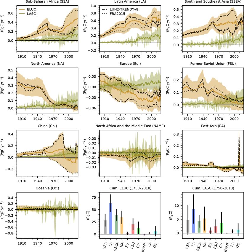
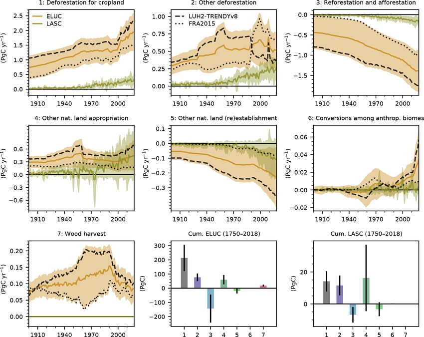
T. Gasser et al.: Historical CO2 emissions from land use and land cover                                                          4083

Figure 4. Regional breakdown of our best-guess estimates. Annual bookkeeping LULCC emissions (in brown) and LASC (in green) are
shown, except in the last two panels where the regional cumulative bookkeeping LULCC emissions (ELUC) and LASC over the 1750–2018
period are shown. Shaded areas and uncertainty bars represent the 1σ uncertainty range. To help identify regional discrepancies between
LULCC driving data sets, we also separate the average estimates for the LUH2-GCB2019 (dashed black line) and FRA2015 (dotted black
line) data sets (which are shown without their own uncertainty for legibility).

in such a case. The noise intensity in Oceania is even larger         3.5   Breakdown by transition
than the signal in any other region, suggesting that some of
the uncertainty in our LASC estimates could be an artifact of         Figure 5 and Table 5 show a breakdown of our global book-
this weakness in our modeling approach. As to the regional            keeping LULCC emissions and LASC following seven cate-
split of the cumulative LASC over the 1750–2018 period, it            gories of LULCC activities. These categories are essentially
roughly follows that of the cumulative LULCC emissions, al-           a subdivision of the main three LULCC activities mentioned
though it is modulated by the land sink’s relative efficiency in      previously in the short description of OSCAR. Category 1
each region. Latin America is the region in which the largest         corresponds to land cover change (LCC) where forest is re-
part of this loss of sink capacity occurred (almost one-third),       placed by cropland. Category 2 is LCC where forest is re-
followed by North America, South and Southeast Asia, and              placed by anything else (but forest). Category 3 is the oppo-
sub-Saharan Africa. However, uncertainties in the LASC are            site of 1 and 2: LCC where any type of land but forest is re-
too high for this ranking to be determined with good statisti-        placed by forest. Category 4 is LCC where non-forested nat-
cal confidence.                                                       ural land is replaced by any anthropogenic land. Category 5

https://doi.org/10.5194/bg-17-4075-2020                                                       Biogeosciences, 17, 4075–4101, 2020
4084                                                  T. Gasser et al.: Historical CO2 emissions from land use and land cover

Table 4. Regional breakdown of bookkeeping LULCC emissions and LASC. This is provided for our best-guess estimates and the two main
LULCC data sets (LUH2-GCB2019 and FRA2015) separately. The regions are defined in Houghton and Nassikas (2017).

                                                  Annual flux 2009–2018 (PgC yr−1 )           Cumulative flux 1750–2018 (PgC)
                                               Best guess            LUH              FRA     Best guess     LUH         FRA
        Bookkeeping LULCC emissions (ELUC)
        Sub–Saharan Africa                   0.46 ± 0.24      0.29 ± 0.11     0.66 ± 0.20        28 ± 13   25 ± 14      31 ± 9
        Latin America                        0.63 ± 0.23      0.52 ± 0.14     0.76 ± 0.24        63 ± 18   67 ± 18     59 ± 17
        South and Southeast Asia             0.32 ± 0.11      0.35 ± 0.09     0.29 ± 0.12        39 ± 12    36 ± 8     42 ± 14
        North America                        0.00 ± 0.04      0.02 ± 0.03    −0.02 ± 0.03        34 ± 13   34 ± 14     35 ± 13
        Europe                              −0.03 ± 0.03     −0.02 ± 0.02    −0.05 ± 0.03          2±3       4±2       −1 ± 2
        Former Soviet Union                  0.01 ± 0.05      0.03 ± 0.03    −0.02 ± 0.05        20 ± 12   20 ± 12     20 ± 12
        China                               −0.05 ± 0.21      0.14 ± 0.07    −0.27 ± 0.05        13 ± 13    23 ± 8       1±5
        North Africa and the Middle East    −0.01 ± 0.01      0.00 ± 0.01    −0.01 ± 0.01        −1 ± 2    −1 ± 2        0±2
        East Asia                            0.00 ± 0.05      0.01 ± 0.04    −0.01 ± 0.01          3±2       4±2           ∼1
        Oceania                              0.03 ± 0.06      0.00 ± 0.04     0.07 ± 0.07         6 ± 10     1±8       11 ± 10
        Loss of additional sink capacity (LASC)
        Sub–Saharan Africa                     0.12 ± 0.13     0.16 ± 0.17     0.08 ± 0.04         5±6       7±7         2±1
        Latin America                          0.18 ± 0.18     0.21 ± 0.21     0.15 ± 0.14         9±5      10 ± 6       7±4
        South and Southeast Asia               0.11 ± 0.08     0.11 ± 0.08     0.11 ± 0.07         4±2       4±3         4±2
        North America                          0.10 ± 0.08     0.11 ± 0.09     0.08 ± 0.07         5±4       6±5         5±4
        Europe                                 0.01 ± 0.02     0.03 ± 0.02     0.00 ± 0.01         1±1       2±1          ∼0
        Former Soviet Union                    0.06 ± 0.06     0.06 ± 0.06     0.05 ± 0.05         2±3       3±3         2±2
        China                                  0.07 ± 0.10     0.12 ± 0.10     0.02 ± 0.07         4±4       5±4         2±3
        North Africa and the Middle East       0.00 ± 0.01     0.00 ± 0.01     0.00 ± 0.01          ∼0         ∼0         ∼0
        East Asia                              0.01 ± 0.01     0.02 ± 0.01          ∼ 0.00         1±1       1±1          ∼0
        Oceania                                0.02 ± 0.11     0.02 ± 0.14     0.03 ± 0.05         1±2       1±3         1±2

Table 5. Breakdown of bookkeeping LULCC emissions and LASC by LULCC activity. This is provided for our best-guess estimates and the
two main LULCC data sets (LUH2-GCB2019 and FRA2015) separately.

                                                  Annual flux 2009–2018 (PgC yr−1 )             Cumulative flux 1750–2018 (PgC)
                                               Best guess           LUH               FRA     Best guess        LUH         FRA
     Bookkeeping LULCC emissions (ELUC)
     Deforestation for cropland              1.86 ± 0.57      2.20 ± 0.48     1.47 ± 0.37      213 ± 93     285 ± 62    131 ± 38
     Other deforestation                     0.55 ± 0.26      0.41 ± 0.14     0.70 ± 0.27       77 ± 27      88 ± 26     64 ± 24
     Reforestation and afforestation        −1.36 ± 0.49     −1.70 ± 0.38    −0.96 ± 0.22     −144 ± 99    −230 ± 48    −45 ± 11
     Other natural land appropriation        0.42 ± 0.31      0.63 ± 0.26     0.17 ± 0.08       60 ± 33      82 ± 30     35 ± 12
     Other natural land (re)establishment   −0.21 ± 0.18     −0.33 ± 0.15    −0.07 ± 0.08      −20 ± 18     −34 ± 11     −3 ± 2
     Conversions among anthrop. biomes       0.02 ± 0.02      0.03 ± 0.02     0.01 ± 0.01         1±1          1±1           ∼0
     Wood harvest                            0.09 ± 0.04      0.10 ± 0.04     0.07 ± 0.03        19 ± 6       21 ± 5      16 ± 6
     Loss of additional sink capacity (LASC)
     Deforestation for cropland              0.29 ± 0.16      0.31 ± 0.17     0.27 ± 0.15         14 ± 6      16 ± 7      12 ± 5
     Other deforestation                     0.24 ± 0.15      0.30 ± 0.15     0.17 ± 0.10         12 ± 6      15 ± 6       7±3
     Reforestation and afforestation        −0.15 ± 0.10     −0.21 ± 0.10    −0.09 ± 0.04        −7 ± 5      −10 ± 4      −3 ± 1
     Other natural land appropriation        0.39 ± 0.53      0.57 ± 0.63     0.19 ± 0.24        16 ± 21     24 ± 25       8±9
     Other natural land (re)establishment   −0.09 ± 0.12     −0.14 ± 0.14    −0.03 ± 0.06        −3 ± 4       −5 ± 5      −1 ± 1
     Conversions among anthrop. biomes       0.00 ± 0.01      0.00 ± 0.01          ∼ 0.00            ∼0          ∼0          ∼0
     Wood harvest                                   0.00             0.00            0.00              0           0           0

Biogeosciences, 17, 4075–4101, 2020                                                         https://doi.org/10.5194/bg-17-4075-2020
T. Gasser et al.: Historical CO2 emissions from land use and land cover 4085 Figure 5. Breakdown of our best-guess estimates by LULCC activities. Annual bookkeeping LULCC emissions (in brown) and LASC (in green) are shown, except in the last two panels that show the regional cumulative bookkeeping LULCC emissions (ELUC) and LASC over the 1750–2018 period. Shaded areas and uncertainty bars represent the 1σ uncertainty range. Similarly to Fig. 3, we also separate the average estimates for the LUH2-GCB2019 (dashed black line) and FRA2015 (dotted black line) data sets (which are shown without their own uncertainty for legibility). is the opposite of 4. Category 6 is any LCC occurring among 213 ± 93 PgC due to deforestation for cropland, 77 ± 27 PgC anthropogenic land (e.g., pasture to cropland). Category 7 is due to other types of deforestation, and 60 ± 33 PgC due to the sum of wood harvest and LCC occurring from any type the loss of other natural land. This was partly compensated of natural land to the same type of natural land (e.g., for- for by −144±99 PgC from reforestation and afforestation as est to forest). Note that the effects of shifting cultivation are well as −20 ± 18 PgC when other natural land was regained. included in their corresponding LCC categories due to the The uncertainty in the bookkeeping LULCC emissions is model’s structure. largely dominated by the discrepancy between the two main Forest-related land cover change dominates historical LULCC data sets. For annual emissions, this is even rein- bookkeeping emissions. Over the last decade, we estimate forced by the fact that shifting cultivation is included in our that an average of 1.86 ± 0.57 PgC yr−1 was emitted due to estimates. Figure A2 indeed shows that both data sets have deforestation in order to establish cropland, an additional a very different level of shifting cultivation area, although 0.55 ± 0.26 PgC yr−1 was from other types of deforestation this is somewhat artificial as it is caused by the difference in (e.g., deforestation for pastoral land or simply due to forest the data sets’ starting year. Therefore, our uncertainty ranges degradation), and a capture of −1.36 ± 0.49 PgC yr−1 was for the deforestation and reforestation categories are over- due to reforestation and afforestation. These estimates in- estimated. For cumulative emissions, however, this overesti- clude the effect of our shifting cultivation driver that en- mation is much lower, as shifting cultivation has a long-term compasses traditional activities such as “slash-and-burn”, effect of zero net emissions in OSCAR (Appendix A7). How- which leads to large but counteracting gross carbon fluxes ever, a few other clear differences between the two data sets caused by back-and-forth deforestation/reforestation activi- remain, such as the opposite trend in 1990 in the “other de- ties (Houghton et al., 2012; Li et al., 2018; Yue et al., 2018). forestation” category or the difference in wood harvest. The cumulative emission over the 1750–2018 period was https://doi.org/10.5194/bg-17-4075-2020 Biogeosciences, 17, 4075–4101, 2020
4086                                                T. Gasser et al.: Historical CO2 emissions from land use and land cover

   When we split the LASC between these transitions types,        pendent and is largely dominated by the biogeochemical un-
we obtain a slightly different picture. Our three categories of   certainty.
natural land appropriation caused roughly similar amounts of
cumulative LASC: 14 ± 6 PgC from deforestation for crop-
land, 15 ± 6 PgC from other deforestation, and 24 ± 25 PgC        4     Discussion
from loss of other natural land. This was partially compen-
                                                                  4.1    The constraint
sated for by a negative LASC (i.e., an increase in the sink ca-
pacity) of −7 ± 5 PgC caused by reforestation and afforesta-      Table 2 shows that the choice of constraint does not drasti-
tion and −3±4 PgC caused by other natural land gain. Other        cally impact our results, as there is a large overlap between
types of LULCC led to a negligible LASC. Regarding the            the estimates obtained with both the old and new constraints.
uncertainty in the LASC, the noise we identified in the pre-      More precisely, LULCC emissions do not show a large im-
vious section can be attributed to the “other natural land”       pact, whereas the land sink and the LASC do. However, this
biome. Combined with the diagnosis from the previous sec-         is somewhat artificial, as both our constraints are aimed at
tion, this suggests that OSCAR may benefit from separating        constraining the processes that dictate the land sink (such as
desert areas (i.e., bare soils) from the non-forest biome. How-   the fertilization effect), which is visible in Fig. 1c where the
ever, this would make processing the LULCC data sets more         unconstrained distribution of the land sink exhibits a large
difficult, as new assumptions should then be made regarding       spread that is reduced after the application of constraints.
how much of this new biome is affected by LULCC.                  Other (or additional) constraints focused on LULCC emis-
                                                                  sions, such as constraints on carbon densities, could be envi-
3.6    Breakdown by carbon pool                                   sioned – although we deemed this unnecessary for this study.
                                                                  Because the constraint is applied after the simulations are
A final axis of analysis that OSCAR can provide is a break-       actually run, it is indeed possible to decide on the best con-
down of the model’s carbon pools, thereby indirectly fol-         straint (or combination thereof) ex post, depending on one’s
lowing its biogeochemical processes. Figure 6 shows such          ultimate goal. Our choice of constraint was driven by our
a breakdown into our three main carbon pools: vegetation          will to make our estimates of LULCC emissions compati-
carbon, soil carbon, and HWPs. Bookkeeping LULCC emis-            ble with the overall GCB2019, our scientific conviction that
sions over the last decade have consisted of a combina-           it is preferable to use physical (i.e., observable) variables as
tion of −3.66 ± 0.96 PgC yr−1 of vegetation carbon (i.e.,         constraints, and our own expert judgement as to which parts
biomass) regrowth, 2.84 ± 0.85 PgC yr−1 emitted by equili-        of the GCB are the most robust. Our choice can be debated,
brating soils, and 2.18 ± 0.65 PgC yr−1 emitted by HWP ox-        however, and we invite the community to download our raw
idization. Here, the equilibration of soils includes both the     estimates and apply their own constraints if they so wish (see
heterotrophic respiration in originally carbon-rich soils that    the “Data availability” section). Ultimately, a Bayesian syn-
is not compensated for by enough primary productivity (e.g.,      thesis framework could be used at the GCB scale (Li et al.,
when deforesting to establish cropland) and the oxidation         2016) to avoid having to make such an arbitrary choice.
of slash products (i.e., dead biomass left on site after land
cover change). The three sub-fluxes have been steadily in-        4.2    The OSCAR model
creasing over the past century or so. Cumulated over the
1750–2018 period, these three pool-specific values amount         OSCAR satisfactorily emulates the carbon densities and
to −443 ± 155, 373 ± 137, and 276 ± 84 PgC, respectively.         stocks of DGVMs (Table A1), but these stocks are in the
   For the LASC, this pool-based decomposition only con-          lower end of existing assessments. The DGVMs we cal-
cerns the vegetation and soil pools, as no HWPs are involved      ibrated OSCAR upon have global preindustrial pools of
in the processes driving the land sink. Both components of        457 ± 77 PgC for vegetation and 1140 ± 336 PgC for soil,
the annual LASC are positive, with notable inter-annual vari-     whereas the IPCC Fifth Assessment Report (Ciais et al.,
ability and positive trend, reaching 0.33 ± 0.25 PgC yr−1 for     2013) gives values of 450–650 and 1500–2400 PgC, respec-
the vegetation and 0.35 ± 0.36 PgC yr−1 for soils, on average     tively. Some of the difference in soil carbon comes from the
over the 2009–2018 period. Over the 1750–2018 period, the         absence of peatland in DGVMs (Nichols and Peteet, 2019),
cumulative component fluxes are 16 ± 7 PgC for vegetation         and some may be explained by the existence of “passive” soil
and 16±16 PgC for soils. These positive values must be inter-     carbon that is not mobilized under the timescales we con-
preted as a storage of carbon that did not occur because the      sider here (Barré et al., 2010; He et al., 2016). Nevertheless,
preindustrial land cover was modified and the new ecosys-         the relatively low carbon pools suggest that our bookkeeping
tems could not provide as strong a land sink as the prein-        LULCC emissions could be underestimated. Alternatively,
dustrial ecosystems. The breakdown shows how this storage         our preindustrial land cover taken from the LULCC data sets
would have been split between vegetation and soil carbon          could be inaccurate (Table A2). We ran the LUH2 data set
pools, had it occurred. Since it is implicitly determined by      starting in 850, and did not find substantial carbon loss be-
the model’s processes, this breakdown is heavily model de-        tween 850 and 1750 (23 ± 15 PgC in total). Other studies

Biogeosciences, 17, 4075–4101, 2020                                                  https://doi.org/10.5194/bg-17-4075-2020
T. Gasser et al.: Historical CO2 emissions from land use and land cover 4087 Figure 6. Breakdown of our best-guess estimates by carbon pools: vegetation (green), soils (brown), and HWPs (red). Shaded areas and uncertainty bars represent the 1σ uncertainty range. that specifically focused on the more distant past have found the model’s parameters depend on the time elapsed since a much higher carbon loss over this early period (Erb et al., given LULCC perturbation (i.e., it has no age classes). For 2018; Kaplan et al., 2011; Pongratz et al., 2008), again sug- instance, 5-year-old forests grow and die at the same rate gesting this part of our results could be underestimated. as 50-year-old forests. This, by construction, means that the A key feature of OSCAR is that the model’s carbon den- biomass regrowth of disturbed ecosystems follows an expo- sities transiently change as a response to changes in en- nential response curve, which we acknowledge is unrealistic. vironmental conditions. This change in carbon densities is The impact of this structural choice is difficult to estimate; fully coupled to the bookkeeping module and, therefore, im- however, as it affects only dynamics and not carbon densities, pacts bookkeeping LULCC emissions. This feature contrasts we can speculate that annual emissions are more impacted with the fixed carbon densities of other bookkeeping mod- than cumulative emissions. Other regrowth curves could be els and makes it possible to account for processes such as introduced (Fekedulegn et al., 1999), although this would CO2 fertilization, wildfire changes, and climate feedbacks. require the introduction of age-dependent functions in the Without any change in environmental conditions, we find model’s formulation, which, in turn, would make it heavier that annual bookkeeping LULCC emissions would have been and slower. Actually, when OSCAR v2.4 was developed, the 1.11±0.35 PgC yr−1 on average over the last decade, and cu- only process that had been age dependent until then, namely mulative emissions would have been 191 ± 52 PgC over the the decay of HWPs (Gasser et al., 2017), was reformulated 1750–2018 period. This is 19 % and 7 % less than our best to be age independent. The reason for this simplification is guesses with environmental changes for the abovementioned that, beyond being a carbon cycle model, OSCAR is also an periods, respectively, and is primarily driven by the lower Earth system model, and the complexity of each of its mod- carbon densities that are caused by the absence of the fertil- ules has to be kept in check. However, it is not excluded that ization effect. The effect on the cumulative emissions is in future variants of the model will see implementation of such line with a previous estimate (Gasser and Ciais, 2013). The a feature. effect on annual emissions, however, is higher. This suggests A final structural element that we find worth mention- that this effect increases with time and will keep increasing ing is the biome aggregation of our model. The final list in the future as environmental conditions change and move of five biomes in OSCAR is a trade-off between the plant further away from preindustrial conditions. This underscores functional types (PFTs) of the DGVMs and the land cover the importance of building hybrid bookkeeping models such classes of the LULCC data sets. Typically, DGVMs tend to as OSCAR that are capable of capturing such an effect. A focus on natural ecosystems (i.e., they have many types of structural limitation of this version of OSCAR is the ab- forests), whereas LULCC data sets focus on anthropogenic sence of any age-specific process. This means that none of ecosystems (i.e., more types of croplands and pastures). Our https://doi.org/10.5194/bg-17-4075-2020 Biogeosciences, 17, 4075–4101, 2020
4088                                                 T. Gasser et al.: Historical CO2 emissions from land use and land cover

list of biomes aimed at limiting the number of assumptions         albeit resource-intensive way of reducing this source of un-
made when processing both types of data for implementa-            certainty. Posterior evaluation and weighting of the DGVMs
tion within OSCAR, but some were necessary nonetheless.            is another approach, be it through a specifically designed pro-
Qualitatively, we see two important caveats caused by our          tocol such as the International Land Model Benchmarking
biome aggregation. First, as we only have one natural biome        (ILAMB) project (Collier et al., 2018) or a synthesis setup
to cover all natural land but forests, we average actual natu-     like ours.
ral ecosystems with relatively high carbon densities such as
shrubland with almost carbon-free ecosystems like deserts.
We saw in previous sections that this may explain part of the
large uncertainty in our LASC estimates, but it likely also af-
fects our bookkeeping LULCC emissions. Second, we do not
distinguish between primary and secondary natural land. In
other words, pristine and disturbed natural ecosystems are as-
sumed to have the same steady-state carbon densities. How-
ever, this does not mean that the actual carbon densities are
the same. It means that it is assumed that, if left undisturbed,
previously disturbed ecosystems will grow back to the exact
same steady state as those that have never been disturbed.
Because they relate to carbon densities, these structural as-
pects are likely to have the largest impact on our estimates.
Quantifying this impact would require a significant amount
of work; however, it would undoubtedly require making new
assumptions that, in turn, would introduce additional uncer-
tainty and potential biases.

5   Conclusions

In spite of those caveats, this study has introduced an in-
novative method to estimate historical LULCC emissions
and LASC, whereby a bookkeeping approach, data from
processed-based models, several LULCC data sets, and an
empirical constraint are consistently combined. We have also
identified key sources of uncertainty that must be reduced
to improve future GCBs. One easy improvement is to de-
cide on where to account for the LASC. We argued else-
where (Gasser and Ciais, 2013) that it is ill-advised to in-
clude the LASC in LULCC emissions, as it is a theoreti-
cal flux that cannot be observed and that does not tend to
zero after LULCC activities cease. However, reducing the
other sources of uncertainty is a more challenging endeavor.
Although satellite data (Hansen et al., 2013) and crowd-
sourcing (Fritz et al., 2019) are currently promising ways of
establishing more accurate land cover maps, these must be
backcast over the past to be relevant for the long-term dy-
namic of the global carbon cycle. Such backcasting gener-
ates new uncertainty (Peng et al., 2017), and additional data,
perhaps in the form of historical records (Bastos et al., 2017;
Houghton and Nassikas, 2017), are required to mitigate the
lack of direct observations. We found that the biogeochem-
ical uncertainty dominated, although that is a reflection of
the uncertainty in the DGVMs’ own parameterization, and
not the uncertainty stemming from direct observations of
real-life carbon densities. Improving the DGVMs’ calibra-
tion (e.g., by assimilating observational data) is an obvious

Biogeosciences, 17, 4075–4101, 2020                                                  https://doi.org/10.5194/bg-17-4075-2020
You can also read