Estimating the probability of compound floods in estuarine regions
←
→
Page content transcription
If your browser does not render page correctly, please read the page content below
Hydrol. Earth Syst. Sci., 25, 2821–2841, 2021
https://doi.org/10.5194/hess-25-2821-2021
© Author(s) 2021. This work is distributed under
the Creative Commons Attribution 4.0 License.

Estimating the probability of compound floods in estuarine regions
Wenyan Wu1,2 , Seth Westra2 , and Michael Leonard2
1 Department    of Infrastructure Engineering, The University of Melbourne, Melbourne, 3010, Australia
2 School   of Civil, Environmental and Mining Engineering, The University of Adelaide, Adelaide, 5005, Australia

Correspondence: Wenyan Wu (wenyan.wu@unimelb.edu.au)

Received: 11 September 2020 – Discussion started: 25 September 2020
Revised: 3 February 2021 – Accepted: 12 April 2021 – Published: 26 May 2021

Abstract. The quantification of flood risk in estuarine re-        ceedance probability flood or 1-in-100-year flood), as well
gions relies on accurate estimation of flood probability,          as for risk-based approaches that consider the integration
which is often challenging due to the rareness of hazardous        of both probability and consequence. Indeed, the estimation
flood events and their multi-causal (or “compound”) na-            of flood probability represents one of the core objectives of
ture. Failure to consider the compounding nature of estuar-        the field of engineering hydrology (Maidment, 1993), with
ine floods can lead to significant underestimation of flood        methodological developments dating back to early flood fre-
risk in these regions. This study provides a comparative re-       quency estimation approaches (Condie and Lee, 1982; Riggs,
view of alternative approaches for estuarine flood estima-         1966; Singh, 1980; Woo, 1971) and the development of rain-
tion – namely, traditional univariate flood frequency analy-       fall intensity–frequency–duration (IFD) curves (Koutsoyian-
sis applied to both observed historical data and simulated         nis et al., 1998; Niemczynowicz, 1982; Yu and Chen, 1996).
data, as well as multivariate frequency analysis applied to           Although many aspects of the flood probability calcula-
flood events. Three specific implementations of the above ap-      tion are strongly supported by theory and embedded in engi-
proaches are evaluated on a case study – the estuarine portion     neering practice (e.g. Ball et al., 2019 and Robson and Reed,
of Swan River in Western Australia – highlighting the advan-       1999), there are several challenges specific to applications in
tages and disadvantages of each approach. The theoretical          estuarine regions that make this a unique category of prob-
understanding of the three approaches, combined with find-         lem. Primary amongst these is that estuarine floods have the
ings from the case study, enable the generation of guidance        potential to be caused by several separate but physically con-
on method selection for estuarine flood probability estima-        nected processes, including high water levels from the ocean
tion, recognizing issues such as data availability, the com-       resulting from storm surge and/or high astronomical tide, as
plexity of the application/analysis process, the location of       well as riverine floods due to intense flood-producing rain-
interest within the estuarine region, the computational de-        fall in the contributing catchments (Couasnon et al., 2020;
mands, and whether or not future conditions need to be as-         IPCC, 2012; Leonard et al., 2014; Zscheischler et al., 2018).
sessed.                                                            In addition, many estuaries around the world and their con-
                                                                   tributing catchments have exhibited substantial changes in
                                                                   land use (e.g. urbanization, agricultural expansion), channel
                                                                   modification (dredging, straightening and damming), coastal
1   Introduction                                                   engineering works and various other modifications (Depart-
                                                                   ment of Climate Change and Energy Efficiency, 2011; Ha-
Estimates of the probability of future floods represent a criti-   bete and Ferreira, 2017; Hallegatte et al., 2013), with the
cal information source for applications such as land-use zon-      implication that historical flood records may provide a poor
ing and planning, reservoir operation, flood protection infras-    guide to future hazard and risk (Milly et al., 2008; Razavi et
tructure design, and dam safety assessments (e.g. Ball et al.,     al., 2020). Climate change adds a further layer of complexity,
2019). Such probability estimates form the basis for calcula-      resulting in increasing ocean levels and changes to storm dy-
tions of the “design flood” (a hypothetical flood with a de-       namics that in turn will lead to changes in both storm surges
fined probability of exceedance, such as the 1 % annual ex-

Published by Copernicus Publications on behalf of the European Geosciences Union.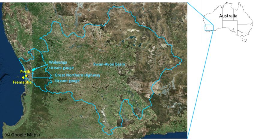
2822                                       W. Wu et al.: Estimating the probability of compound floods in estuarine regions

and rainfall patterns (Lowe and Gregory, 2005; Wasko and            mechanism arises through the combination of astronomic
Sharma, 2015; Westra et al., 2014) as well as their depen-          tides and a set of meteorological processes (e.g. tropical or
dence (Ganguli and Merz, 2019; Wahl et al., 2015; Wu and            extra-tropical cyclones) that produce onshore winds and an
Leonard, 2019). The combination of these factors means that         inverse barometric effect, which in turn leads to storm surges
conventional approaches for flood risk estimation as com-           and strong waves. The magnitude, timing and duration of el-
monly applied to inland catchments are rarely suitable for          evated oceanic water levels due to this mechanism depend on
estuarine situations (Couasnon et al., 2020; Zscheischler et        the dynamics (e.g. timing and duration) of the storm surge,
al., 2018).                                                         its superposition on the astronomic tide (i.e. the interaction of
   To illustrate these challenges, consider Typhoon Ramma-          surge and tide, with the greatest effects during spring tides;
sun, in which intense rainfall combined with storm surge pro-       Cowell and Thom, 1995) and various bathymetric effects that
duced a compound flood. As one of only two Category 5               influence propagation of the flood wave up the estuary (Resio
super typhoons recorded in the South China Sea, Typhoon             and Westerink, 2008; Wu et al., 2017).
Rammasun made landfall at its peak intensity over the is-              Although these two physical processes are often treated
land province of Hainan in China on 18 July 2014. It brought        separately, the flood level within an estuary is not a sim-
both heavy rainfall and a strong surge with return periods          ple addition of a fluvial hydrograph and an elevated coastal
of more than 100 years to the city of Haikou, the capital           water level (Bilskie and Hagen, 2018; Ikeuchi et al., 2017;
of Hainan province located on the estuary of Nandu River            Santiago-Collazo et al., 2019). In particular, complex estu-
(Xu et al., 2018). Heavy rain caused widespread flooding            arine hydrodynamics need to be considered, and the poten-
in Haikou city and nearby urban areas. Storm surge over             tial for coincident or offset timing of each component (in
3 m was observed on the northern coast of the island, which         terms of the coincidence between the arrival of the hydro-
prevented water from the Nandu River from draining into             graph peak, the storm surge peak and the interaction with
the sea, further exacerbating the impacts of floods in and          tidal cycles) can add considerable complexity to probabil-
nearby Haikou city (Wang et al., 2017). Yet flood estimation        ity calculations. Furthermore, the meteorological drivers are
in this region proved problematic (Wang et al., 2017; Xu et         sometimes (but not always) common between heavy rain-
al., 2018): historical flood records are short; the region has      fall events and storm surges, such that the catchment and
experienced rapid and extensive urbanization including sig-         oceanic processes that drive estuarine floods can exhibit a
nificant hydraulic changes in Nandu River leading to non-           non-negligible probability of occurring simultaneously (Be-
stationarity, and climate change is already modifying key           vacqua et al., 2017; Leonard et al., 2014; Wahl et al., 2015;
flood-generating processes such as mean sea level and heavy         Wu et al., 2018; Zheng et al., 2015a; Zscheischler et al.,
rainfall (IPCC, 2012). This is not an isolated example; with        2018). Methods that explicitly address this compounding be-
large human populations situated at low elevations in close         haviour have only started to be developed relatively recently
proximity to where rivers meet the ocean, there are many            (Zscheischler et al., 2020).
cases where interacting processes lead to complex flood dy-            To address this complexity and provide credible estimates
namics and substantial impacts (e.g. Hanson et al., 2011;           of flood probability in estuarine regions, it is necessary to
Couasnon et al., 2020). On top of this, recent studies show         make methodological decisions based on factors including
that the joint probability of flood drivers in estuarine areas is     – the dominant processes that have the greatest potential
affected by low-frequency climate variability, such as due to
                                                                        to produce estuarine flooding;
the El Niño–Southern Oscillation (Wu and Leonard, 2019),
and may also be experiencing long-term changes (Arns et al.,          – the extent to which key coastal, estuarine and/or catch-
2020; Bevacqua et al., 2019), making it a more challenging              ment properties (e.g. land-use change and hydraulic
task to estimate future flood risk in these areas.                      structures) have changed or are anticipated to change
   A generalized schematic for how the flood-producing pro-             in the future;
cesses interact in an estuarine region is provided in Fig. 1.
                                                                      – the extent to which key meteorological and climatic
Conceptually, elevated estuarine water levels are often repre-
                                                                        drivers have changed or are anticipated to change in the
sented as the combined effect of two separate mechanisms.
                                                                        future;
The first mechanism arises from extensive rainfall occurring
in the upstream catchments, leading to elevated riverine flows        – the availability of data on either historical flooding in
and high water levels in the lower catchment reaches. The               the estuary and/or data on the dominant flood drivers;
magnitude, timing and duration of the ensuing flood wave                and
driven by this mechanism depends on a combination of me-
teorological factors (e.g. intensity, duration and spatial ex-        – a range of other factors (e.g. availability of numerical
tent of the flood-producing rainfall event) and catchment at-           models, methodological expectations articulated in en-
tributes (e.g. size, topography, the wetness of the catchment           gineering guidance documents, available budget) that
prior to the flood-producing rainfall event, and other fac-             ultimately will have a significant bearing on method se-
tors influencing the rainfall–runoff relationship). The second          lection.

Hydrol. Earth Syst. Sci., 25, 2821–2841, 2021                                        https://doi.org/10.5194/hess-25-2821-2021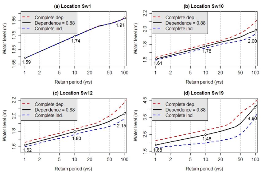
W. Wu et al.: Estimating the probability of compound floods in estuarine regions                                                 2823

Figure 1. Processes that commonly lead to flooding in estuarine regions with common meteorological drivers such as wind and the inverse
barometric effect. Extreme rainfall can cause significant streamflow events in upstream or local urban regions, which may combine with
elevated ocean levels at the lower estuarine boundary. The specific flood magnitude depends on the timing and magnitude of constituent
processes.

The purpose of this paper is to provide a detailed conceptual         use of a probability distribution (often, but not always, an
overview of the broad approaches for estimating the prob-             extreme value distribution) to convert historical and/or simu-
ability of compound floods in estuarine regions and to re-            lated flood records or their drivers into an exceedance proba-
view a set of specific methods available from each approach,          bility. In defining the typology, three general approaches for
given availability of data, calibrated models and computa-            the probability calculation have been identified and consid-
tional power. Advantages and disadvantages of a subset of             ered here:
these methods are then illustrated using a real-world case
study of an estuarine river system in Australia.                        – Approach 1 – univariate flood frequency analysis ap-
   The rest of the paper is organized as follows. A typology              plied directly to observed compound flood data;
of three approaches for estimating the probability of flood
                                                                        – Approach 2 – univariate flood frequency analysis ap-
in estuarine regions is provided in Sect. 2. A description of
                                                                          plied to simulated compound flood data; and
the case study area and data used in this study is provided in
Sect. 3. Details a set of specific methods selected from the            – Approach 3 – multivariate frequency analysis applied to
three approaches and how they are applied to the case study               key compound-flood-generating processes.
are provided in Sect. 4. The flood estimates produced by ap-
plying the selected methods to the case study are summa-                 These approaches are defined by two key methodologi-
rized in Sect. 5. The discussion of main findings is included         cal decisions. The first decision is the extent to which key
in Sect. 6, followed by conclusions in Sect. 7.                       processes need to be explicitly resolved through numerical
                                                                      models or are embedded as stationary boundary conditions.
                                                                      In the first approach (i.e. univariate flood frequency analy-
2     A typology of approaches for estimating the                     sis applied to observed flood data), all the physical processes
      probability of estuarine floods                                 that have led to the historical flood record are embedded in
                                                                      the observed flood data, and thus no physical modelling is
2.1    Background                                                     required. In contrast, the remaining approaches all involve
                                                                      some level of numerical or statistical modelling of the key
A typology of different approaches for estimating estuarine           physical processes that lead to flooding, albeit with signif-
flood probability is given in Fig. 2. Given the requirement           icant differences in the specific models used to implement
for probability estimation, common to all approaches is the           the approaches and the manner in which they are combined.

https://doi.org/10.5194/hess-25-2821-2021                                          Hydrol. Earth Syst. Sci., 25, 2821–2841, 2021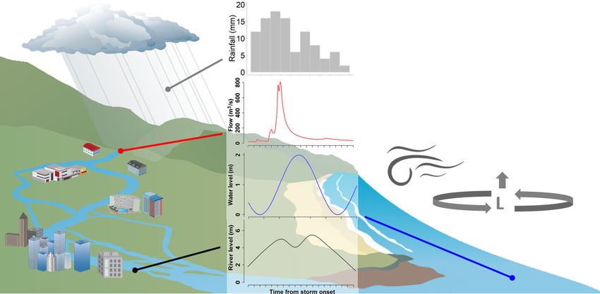
2824                                          W. Wu et al.: Estimating the probability of compound floods in estuarine regions

Figure 2. Pathways for relating process modelling and statistical modelling to determine extremal water levels in estuarine river reaches,
where the top-left panel shows typical system boundaries for identifying relevant modelling domains (atmospheric, hydrological, oceano-
graphic and riverine hydrodynamic) as well as key variables crossing between model domains (R – rainfall, P – pressure, W – wind, Q –
streamflow/river discharge, H – tailwater height in the ocean). Pathway 1: first transform variables to water level via continuous time-stepping
process models and then apply univariate frequency analysis. Pathway 2: first abstract the system to multivariate events represented via mul-
tivariate frequency analysis and then apply the design event process model to derive the compound flood water levels and their corresponding
probability of exceedance.

Each of the modelling approaches therefore requires identi-               merically simulated flood data (Approach 2). The univari-
fication of a modelling domain and a set of boundary con-                 ate probability calculation is illustrated in Fig. 2 by moving
ditions that delineate this domain (top-left panel of Fig. 2).            from the bottom-left panel to the bottom-right panel. Ap-
These boundary conditions may trace back to the meteoro-                  proach 2 requires the additional step of using continuous
logical drivers (e.g. barometric pressure and wind data that              or censored continuous simulation models to move from the
would inform ocean models such as ROMS, Shchepetkin and                   top-left panel of Fig. 2 (describing the physical processes to
McWilliams, 2005; or rainfall data that would inform hydro-               be simulated) to the bottom-left panel (providing the con-
logical models to convert rainfall to flow) or to some inter-             tinuous or censored continuous sequences of flood levels or
mediate variable(s) such as the historical ocean levels and/or            similar flood metrics), before conducting the univariate prob-
historical fluvial flows that represent inflows to the estuary            ability calculation. In contrast, Approach 3 applies multivari-
(Chu et al., 2020; Xie et al., 2021).                                     ate probability approaches further up the modelling chain to
   The second decision is the point at which a probability                define multivariate design events (shifting from the top-left to
model is applied (i.e. directly to the variable of interest, such         top-right panel in Fig. 2), which are then converted to flood
as flood height at a critical location, or to the drivers of flood-       levels by dynamically modelling the individual multivariate
ing some distance up a modelling chain). Approaches 1 and 2               design events (top right to bottom right in Fig. 2).
both apply a univariate probability model directly to the flood              The three primary approaches are described further in the
data (e.g. flood level) at the location of interest, with the dif-        sections below. Within each approach there is significant va-
ference between them being whether the probability model                  riety in terms of specific methods and modelling assumptions
is applied to observed historical data (Approach 1) or nu-

Hydrol. Earth Syst. Sci., 25, 2821–2841, 2021                                                https://doi.org/10.5194/hess-25-2821-2021
W. Wu et al.: Estimating the probability of compound floods in estuarine regions                                               2825

used, and a detailed review is provided for alternative imple-            engineering works, natural littoral drift and fluvial sed-
mentations for each approach.                                             iment transport processes) and/or the upstream catch-
                                                                          ment (e.g. urbanization, agricultural expansion, reser-
2.2   Approach 1: univariate flood frequency analysis                     voir construction, channel modification) can mean that
      applied to observed flood data                                      the historical flood record may be a poor guide to future
                                                                          flood probabilities.
Arguably the simplest approach is the application of a uni-
variate probability model to observed historical flood data at        – Historical and/or future changes to the atmospheric and
the location of interest. This method is well developed (Rob-           oceanic drivers of flooding due to climate change, in-
son and Reed, 1999) and requires sufficient historical data (to         cluding sea level rise, storm surge and changes to rain-
ensure sufficient accuracy in flood estimates, with a typical           fall patterns, can also result in the historical record being
rule of thumb being the requirement of at least 30 years to             a poor guide to future flooding.
estimate flood levels corresponding to probabilities up to the
                                                                    As a result of these limitations, traditional univariate flood
1 % annual exceedance probability; Ball et al., 2019). Once
                                                                    frequency analyses applied to observed historical flood data
these data are obtained, a univariate probability model is ap-
                                                                    are rarely directly appropriate for estimates of future proba-
plied, usually to annual maxima or block maxima time series
                                                                    bilities of estuarine flooding (Yu et al., 2019), and thus one of
of water levels (Bezak et al., 2014; Machado et al., 2015;
                                                                    the alternative approaches outlined below will be required for
Wright et al., 2020). As such there is no explicit physical
                                                                    most real-world applications. Note that in situations where
modelling of any constituent processes; rather, all the physi-
                                                                    historical records of estuarine flooding levels are available,
cal processes are considered to be embedded in the observed
                                                                    these data are still likely to be highly valuable to help cali-
historical flood data.
                                                                    brate numerical models and/or otherwise benchmark proba-
   A key assumption is that the physical generating processes
                                                                    bility calculations.
that gave rise to this historical record of flooding will con-
tinue into future floods (in a statistical sense), so that the      2.3   Approach 2: univariate flood frequency analysis
probability distribution fitted to the historical data can be as-         applied to simulated flood data
sumed to be stationary. Although there are many benefits to
this approach – including its simplicity and transparency –         The second approach (tracing from the top-left panel to the
there are a number of limitations.                                  bottom-left panel and then to the bottom-right panel in Fig. 2)
                                                                    is often referred to as “continuous simulation” and involves
  – Historical gauges are rarely available precisely at the
                                                                    simulating the dynamical flood response to continuous time
    location(s) of interest within an estuary, with the com-
                                                                    series of the modelling boundary conditions using process-
    plexity of flood wave attenuation throughout estuarine
                                                                    based models (Boughton and Droop, 2003; Sopelana et al.,
    systems making it problematic to simply extrapolate in-
                                                                    2018). For example, if extended continuous historical data of
    formation from one location to the next without con-
                                                                    catchment inflows (upper boundary condition) and ocean lev-
    sideration of the hydrodynamic processes. The lack of
                                                                    els (lower boundary condition) are available, then it becomes
    gauges within estuaries is likely to be at least in part due
                                                                    possible to run a hydrodynamic model forced by those con-
    to the fact that there has historically been greater interest
                                                                    ditions to achieve continuous water level time series at all
    in measuring either the sea level or the river discharge,
                                                                    relevant locations within the estuary. This in turn can form
    and therefore there is less interest to place stations at the
                                                                    the basis of a univariate flood frequency analysis applied to
    interface between the two (Bevacqua et al., 2017).
                                                                    the simulated flood level data at the location(s) of interest.
  – Frequency approaches are more commonly applied to               An advantage of this approach is that flood levels can be cal-
    flood volume (i.e. flow) data rather than flood water           culated at all desired locations throughout the estuary and
    level data, which can be problematic in estuarine re-           that changes within the estuary (e.g. changes in bathymetry,
    gions where flows can be bidirectional and water levels         engineering works) can be explicitly captured in the model.
    are influenced by both upstream and downstream pro-             However, the approach assumes that the physical generating
    cesses.                                                         processes that lead to the boundary conditions are and will
                                                                    continue to be stationary, which is increasingly unlikely to
  – Complex bathymetry and other physical features of es-           be valid for a range of applications.
    tuarine flooding make it difficult to extrapolate the fre-         A possible solution for addressing boundary condition
    quency curve when using observed historical records             non-stationarity is to widen the modelling chain, thereby ex-
    to estimate rare design events that are greater than the        plicitly representing a broader range of physical processes
    largest observed flood.                                         in the model (Heavens et al., 2013). For example, land-use
                                                                    change or the construction of a reservoir in the upstream
  – Historical and/or future changes to either the estuary it-      catchment can lead to significant non-stationarity in stream-
    self (e.g. changes to bathymetry due to dredging, coastal       flow time series (the upper boundary condition in the pre-

https://doi.org/10.5194/hess-25-2821-2021                                         Hydrol. Earth Syst. Sci., 25, 2821–2841, 2021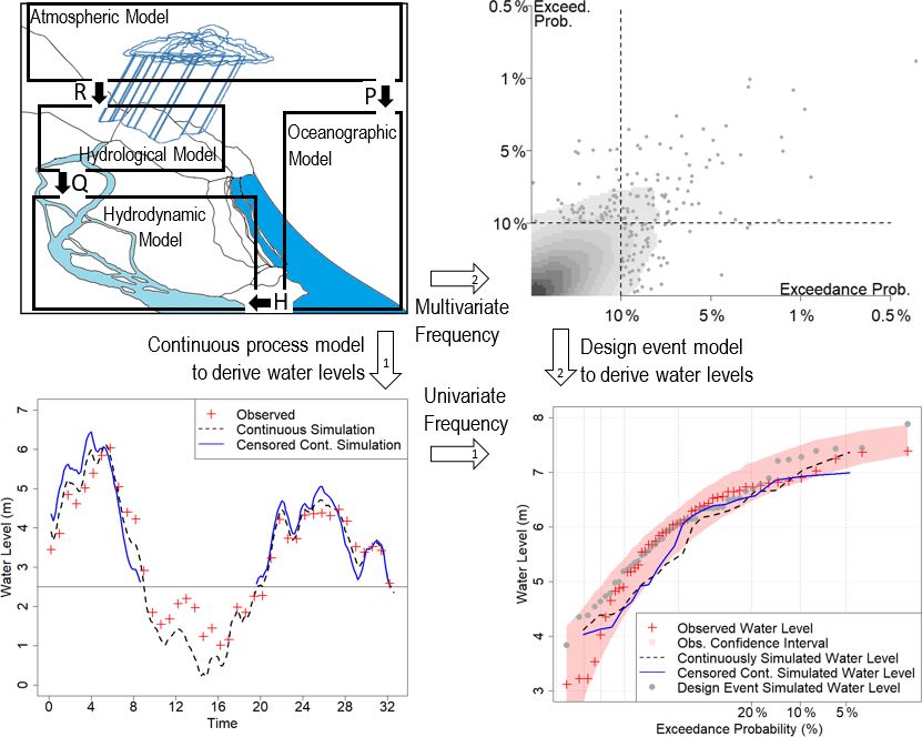
2826                                     W. Wu et al.: Estimating the probability of compound floods in estuarine regions

ceding example), and this could be addressed by extending         of how to correctly apply continuous simulation approaches
the boundary condition further up to time series of histori-      to estuarine floods remain an open research question.
cal rainfall (Hasan et al., 2019). From there it becomes pos-
sible to explicitly model the key flow-generation processes       2.4   Approach 3: multivariate frequency analysis
(including the effects of land-use change and/or reservoirs)            applied to key flood-generating processes
before coupling this to a hydrodynamic model of the estuary.
This would enable continuous flood height data in the estuary     The third approach involves the application of multivariate
to be generated based on current or future catchment condi-       probability distributions and is often referred to as “event
tions (which would need to be parameterized into the hydro-       based” because of the emphasis on deriving a series of mul-
logical and hydraulic models), forced in this case by histori-    tivariate design events for further simulation through a mod-
cal rainfall time series. Although this approach explicitly ad-   elling chain. These approaches are the multivariate analogy
dresses some sources of non-stationarity, evidence of climate     of applying IFD curves for delineating design rainfall events
change shifting both rainfall patterns and storm surge pat-       with pre-defined probabilities, which are then converted into
terns (Lowe and Gregory, 2005; Wasko and Sharma, 2015;            streamflow events that are assumed to have equivalent prob-
Westra et al., 2014) means that the assumption of station-        ability to the driving rainfall event.
ary meteorological forcing is also increasingly questionable.        These methods factorize the flood estimation problem into
Addressing this issue would lead to further widening of the       two separate components:
boundary conditions. This is represented as ever larger boxes       1. the estimation of a multivariate (commonly bivariate)
in the top-left panel of Fig. 2, defining the components of the        probability distribution function based on the continu-
system to be modelled and the boundary conditions to those             ous boundary conditions; and
models. Widening the modelling chain to explicitly represent
an ever-increasing set of time-varying processes is certainly       2. the estimation of the flood magnitude (i.e. water lev-
an attractive means to explicitly address the non-stationarity         els) for each combination of boundary conditions, us-
of key flood-generating processes. This is especially the case         ing what is often referred to as a “structure variable” or
considering that some datasets from climate models already             “boundary function”.
exist as boundary conditions for hydrodynamical modelling
runs (e.g. Kanamitsu et al., 2002; Naughton, 2016), which         A range of multivariate approaches have been applied to
are helpful to assess climate change impact on compound           compound flood estimation problems, including vine cop-
flooding with Approach 2. However, it is important to rec-        ula (Bevacqua et al., 2017), standard copulas (Muñoz et al.,
ognize that widening the modelling chain can also lead to         2020), unit Fréchet transformations (Zheng et al., 2014), re-
evermore complex models, with greater possibility of induc-       gression type models (Serafin et al., 2019) and conditional
ing biases and other forms of modelling errors into the re-       exceedance models (Jane et al., 2020). The use of copu-
sults (Zaehle et al., 2011). This is particularly the case for    las or equivalent formulations (e.g. unit Fréchet transforma-
climate model outputs, with the lack of hydrological validity     tions) enables the factorization of multivariate distributions
of precipitation fields from climate models often leading to      into a set of marginal distributions and a dependence struc-
the requirement for significant bias correction or other forms    ture (i.e. a joint probability distribution). This joint probabil-
of post-processing (e.g. Nahar et al., 2017).                     ity distribution captures the defining features of the variables
   Furthermore, in the context of estuarine applications, the     of interest and their interaction. For example, in Australia,
implications of anthropogenic climate change mean that it         a bivariate logistic extreme value distribution has been fitted
may be necessary to explicitly resolve the multivariate me-       to tide (observed and simulated) and rainfall data through-
teorological forcing variables that drive estuarine floods. Yet   out the Australian coastline, and the dependence parameter
very little research has been conducted on the generation of      of this distribution has been made available to flood practi-
continuous multivariate meteorological forcing variables for      tioners across the entire coastline to describe the dependence
estuarine catchments while preserving the interactions be-        between storm tide levels and extreme rainfall (Wu et al.,
tween these variables (e.g. the joint probability of extreme      2018; Zheng et al., 2014). To capture the full joint distribu-
rainfall and the meteorological drivers of storm surge such       tion (including both marginal distributions), the dependence
as pressure and wind) and eliminating their respective bi-        parameter can be coupled with publicly available IFD curves
ases. Although approximate approaches may be available in         that capture the rainfall exceedance probabilities of equiva-
certain instances (e.g. manually scaling the rainfall or storm    lent durations and with a frequency analysis of storm tide to
surge boundary conditions), the complexity of possible fu-        reflect the lower boundary condition (Ball et al., 2019). Sim-
ture changes (e.g. heavy rainfall events being more likely to     ilar approaches exist elsewhere (e.g. Bevacqua et al., 2017;
coincide with storm surge events in the future; see Senevi-       Zellou and Rahali, 2019; Moftakhari et al., 2019), and meth-
ratne et al., 2012, and Bevacqua et al., 2019) could render       ods are available to estimate all the key parameters of a suit-
simple scaling approaches invalid. Therefore, many aspects        able distribution when the relevant parameters are unavail-
                                                                  able.

Hydrol. Earth Syst. Sci., 25, 2821–2841, 2021                                      https://doi.org/10.5194/hess-25-2821-2021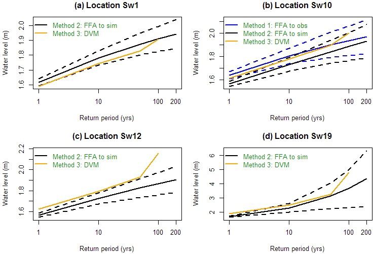
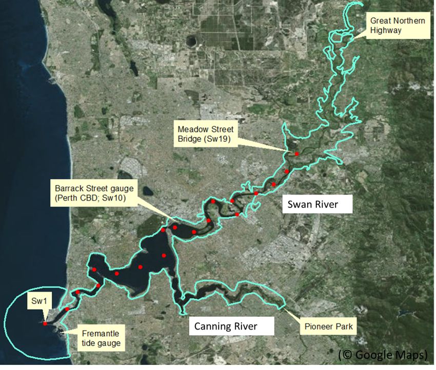
W. Wu et al.: Estimating the probability of compound floods in estuarine regions                                              2827

   There are several advantages of taking an event-based             ing to align the timing of the storm surge and astronomical
approach. First, because of the emphasis on simulating a             tide events with the timing of the flood-producing rainfall in
smaller number of significant design events, the computa-            the upstream catchments (Santiago-Collazo et al., 2019). In-
tional loads are much lower than multi-year continuous simu-         deed, this problem has not been resolved, with most current
lations of hydrodynamic models. Second, because the drivers          methods using a stochastic method to account for the tempo-
of estuarine flooding are factorized through the multivariate        ral shape of surge peaks (MacPherson et al., 2019) or taking a
distribution, it becomes easier to incorporate the effects of        simplified approach such as assuming static lower boundary
future changes. This is particularly the case if one is able to      conditions rather than explicitly resolving the tidal dynamics
assume either that the dependencies between variables are            (Zheng et al., 2015a). The extent to which this simplification
not greatly affected by climate change or that changes in de-        leads to mis-specified flood risk (and whether this misspeci-
pendencies produce second-order effects on flood probability         fication leads to an under- or overestimation of probabilities)
compared to changes in the marginal distributions (Bevacqua          is not known.
et al., 2020). Under these conditions, the method can capital-
ize on published information on uplift factors to changes in
the key marginal distributions (e.g. scaling factors for IFD         3     Case study and data
curves, or for peak ocean levels), which are becoming in-
creasingly commonly available as part of engineering flood           3.1    Case study area and hydrodynamic model
guidance in many parts of the world (Wasko et al., 2021). A
further advantage is that under the assumption that the rel-         The case study is the Swan River system in the lower part
ative timing of different flood drivers is not considered (see       of the Swan–Avon basin in Western Australia, as shown in
discussion in the paragraph below), the flood surface pro-           Fig. 3. The total catchment area of the Swan–Avon River
duced using hydrodynamic models will not change under cli-           system is approximately 124 000 km2 , which makes it one
mate change; rather it is how the flood surface is converted         of the largest river basins in Australia. The river system runs
into flood probability based on the dependence model that            from the town of Coolgardie 500 km east of Perth to its out-
will change. Indeed, by separating the flood estimation prob-        let to the Indian Ocean at Fremantle. The catchment covers a
lem into the two components indicated above (i.e. flood sur-         large proportion of the south-western region of Western Aus-
face and associated probability), it could be possible under         tralia and consists of a wide range of hydrological regimes
certain conditions to estimate the impact of future changes          and land uses, including the relatively wet and forested areas
such as climate change on estuarine flooding without addi-           of the Darling Scarp in the west, the Wheatbelt in the mid-
tional hydrodynamic simulations, simply by re-calculating            dle and the semi-arid Goldfields region in the east. Due to
the probabilities of the flood drivers and their dependence          its large size and hydrological complexity, there is currently
structure under changed future conditions.                           no hydrological model available for the catchment. However,
   Despite these advantages, there are several simplifications       there are a few streamflow gauges near the outlet of the catch-
involved in this approach when converting continuous mete-           ment but outside of the zone of tidal influence. These gauges
orological data into a set of multivariate design events, which      include the Walyunga stream gauge and the Great Northern
could lead to significant misspecification of flood probability      Highway stream gauge and are shown in Fig. 3.
if not taken into account. This is illustrated through an anal-         The case study area is shown in Fig. 4, which covers Swan
ogy of the application of IFD curves to estimate design flood        River from the Great Northern Highway Bridge to its out-
hydrographs, whereby the process of calculating IFD curves           let at Fremantle. A two-dimensional flexible mesh hydro-
involves collapsing complex rainfall events into average rain-       dynamic model is available for the study area. The model
fall intensities for different durations, resulting in the loss of   was developed using the DHI modelling suite MIKE21 by
the spatial and temporal dynamics of individual storm events.        URS on behalf of the Department of Water and Environmen-
To convert IFDs into design floods, this additional temporal         tal Regulation in Western Australia to simulate water levels
and spatial information of the rainfall event is then typically      within the Swan and Canning rivers’ estuarine region (URS,
re-introduced through temporal patterns and areal reduction          2013). The model domain extends from Fremantle to the
factors, respectively. Translating this analogy to multivariate      Great Northern Highway Bridge 40 km north-east of Perth
design events for estuarine conditions, intensity–frequency          on the Swan River and the Pioneer Park gauge station 20 km
relationships for storm tides are often derived from time se-        south-east of Perth on the Canning River. The main area of
ries of daily maximum storm tide. During this process infor-         interest is the Swan River between Fremantle and Meadow
mation on the temporal dynamics of storm surges and astro-           Street Bridge, where model results are most representative of
nomical tides is discarded. Although it may be possible to           historical calibration events (URS, 2013). Therefore, 19 lo-
introduce this information on oceanographic temporal pat-            cations are marked within this region and labelled from Sw1
terns through the use of basis functions such as applied by          at Fremantle to Sw19 at Meadow Street Bridge (represented
Wu et al. (2017) or a similar approach by the UK Environ-            by red dots in Fig. 4), where flood level results are extracted
ment Agency (2019), a significant difficulty arises when try-        from the model. The downstream boundary of the MIKE21

https://doi.org/10.5194/hess-25-2821-2021                                         Hydrol. Earth Syst. Sci., 25, 2821–2841, 2021
2828                                        W. Wu et al.: Estimating the probability of compound floods in estuarine regions

Figure 3. Locations of Perth, Fremantle, Great Northern Highway and Walyunga stream gauges, and Swan–Avon basin. The yellow dots
represent the locations of major urban areas, and the blue dots represent the locations of the stream gauges. (This figure was created using
© Google Maps.)

model is an offshore arch-shaped water level boundary lo-
cated 4 km from Fremantle. The upstream boundaries are
located at the Great Norther Highway Bridge on the Swan
River and Pioneer Park on the Canning River. The region
downstream of Sw10 is mainly storm tide dominated, the re-
gion upstream Sw16 (near the Perth Airport) is mainly flow
dominated, and the region between Sw10 and Sw16 has sig-
nificant joint impact from both tailwater levels at Fremantle
and upstream flow and therefore is referred to as the “joint
probability zone” or “transition zone”.

3.2    Observed data available

Water level data (i.e. not flow volume) within the estuarine
regions of the Swan River are available at one gauge located
at the end of Barrack Street in the city of Perth (near loca-
tion Sw10 in Fig. 4). The data are available from the Depart-
ment of Transport, Western Australia, between July 1990 and
June 2015 at 15 min intervals with approximately 10 % miss-             Figure 4. Model extent and key locations for the case study system.
ing or erroneous values. This leads to about 22 years of data           The blue line represents hydrodynamic model extent. The red dots
with no missing or erroneous values and with water levels               represent the 19 locations where flood level results are extracted,
                                                                        from Sw1 at Fremantle to Sw19 at Meadow Street Bridge. (This
ranging from 0.06 to 1.92 m.
                                                                        figure was created using © Google Maps.)
   Sea level data at Fremantle are available at hourly inter-
vals for 118 years between 1897 and 2015 from the Bureau
of Meteorology, with about 10 % missing or erroneous data.
The sea level data represent the combined influence of astro-           way Bridge gauge are available for 14 years between 1996
nomical tides, storm surge, and other factors that have an im-          and 2010, which is considered to be too short for analysis of
pact on ocean water levels and therefore are also referred to           extreme events. Consequently, streamflow data from the Wa-
as storm tide. The recorded sea levels range between 0.1 and            lyunga gauge, available between 1970 and 2016, are used.
1.95 m.                                                                 The Walyunga gauge is about 4 km upstream of the Great
   Hourly streamflow data from both the Walyunga and the                Northern Highway Bridge, and this distance is considered to
Great North Highway Bridge gauge stations are obtained                  have minimal impact on model results considering the size of
from the Department of Water and Environmental Regula-                  the catchment. After removing missing and erroneous data,
tion, Western Australia. Data from the Great North High-                there are in total 31 years of data available. No streamflow

Hydrol. Earth Syst. Sci., 25, 2821–2841, 2021                                             https://doi.org/10.5194/hess-25-2821-2021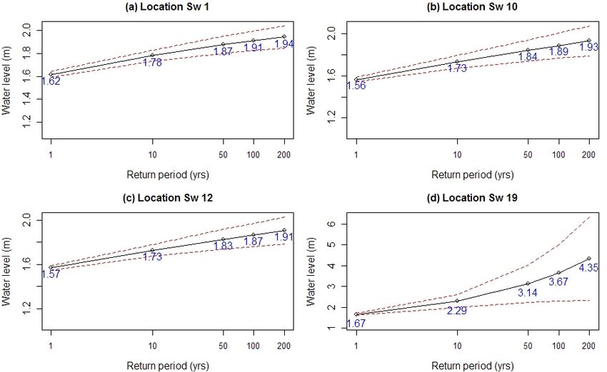
W. Wu et al.: Estimating the probability of compound floods in estuarine regions                                                  2829

data are available for the Canning River. This is not consid-          One challenge associated with a GPD-based frequency
ered a problem, as the inflows upstream of the Canning River        analysis is the choice of the threshold value u. If the thresh-
have little impact on water levels within the study area along      old value is too low, it will violate the basic asymptotic as-
the Swan River (URS, 2013). Consequently, a constant small          sumption of the peak-over-threshold model and lead to high
flow of 1 m3 s−1 is used as the boundary condition at Pioneer       bias in estimation. On the other hand, if the threshold value
Park (URS, 2013).                                                   is too high, there will be insufficient data for fitting the distri-
                                                                    bution, which can lead to high variance. The basic principle
                                                                    for threshold selection is to choose as low a threshold value
4     Methodology                                                   as possible that does not invalidate the asymptotic assump-
                                                                    tion of the model. In this study, the commonly used mean
As described in Sect. 2, each of the general approaches to
                                                                    residual life (MRL) plot method (Coles, 2001) is used for
the estimation of estuarine flood probabilities can be imple-
                                                                    threshold value selection. At the suitable threshold value, the
mented in many different ways, and one specific method is
                                                                    MRL plot should be approximately linear as a function of
applied on the real-world case study to demonstrate the ad-
                                                                    threshold value u (Coles, 2001).
vantages and disadvantages of each approach. The details of
these specific methods and how they are implemented over
                                                                    4.2   Method 2: peak-over-threshold-model-based flood
the case study are presented in this section.
                                                                          frequency analysis applied to simulated flood data
4.1    Method 1: peak-over-threshold-model-based flood
       frequency analysis applied to observed flood data            For Approach 2, univariate flood frequency analysis is ap-
                                                                    plied to flood level data simulated using a 2D hydrodynamic
Univariate flood frequency analysis is the simplest approach        model. To be consistent with the method selected for Ap-
for estimating flood probabilities when flood data are avail-       proach 1, the GPD is also used. One advantage of using the
able, and this method has been used extensively in previous         peak-over-threshold model for Approach 2 is that censoring
studies (Guru and Jha, 2016; Seckin et al., 2014; Xu and            can be used to improve the efficiency of full continuous simu-
Huang, 2011; Zhang et al., 2017). It generally involves fit-        lation using a 2D hydrodynamic model, as only values above
ting a specified distribution (e.g. Gumbel distribution, log-       certain high thresholds need to be included as part of the
Pearson type III distribution or generalized extreme value          joint probability calculation. This assumption is also based
distribution) to flood data so that the magnitude of floods         on the fact that floods are relatively rare events, and there-
can be associated with their occurrence probability (Tao and        fore data from the majority of the record will not be used to
Hamed, 2000). For this study the peak-over-threshold repre-         estimate the probability of floods. Therefore, it is more ef-
sentation of extremes is used.                                      ficient to only simulate water levels above an appropriately
   The peak-over-threshold representation for extreme value         high threshold value, which will reduce simulation time sig-
analysis is based on the Pickands–Balkema–de Haan the-              nificantly.
orem, which leads to the generalized Pareto distribu-                  The censored continuous simulation for generating com-
tion (GPD) family (Coles, 2001). Let {X1 , X2 , . . . , Xn } be a   pound flood levels resulting from tailwater level T and river
sequence of independent and identically distributed random          discharge Q is illustrated in Fig. 5. By selecting all of the
variables that follow a generalized extreme value (GEV) dis-        time periods when at least one of the boundary conditions
tribution:                                                          is above the pre-determined threshold, this approach aims to
             (                         )                           simulate all water levels H above a specified high threshold
                          x − µ −1/ξ

                                                                    value. One challenge to implementing this approach is that it
G(x) = exp − 1 + ξ                        ,                   (1)
                            σ                                       is not possible to know a priori (i.e. without simulating the
                                                                    full time series of joint boundary conditions) the exact value
where µ, σ > 0 and ξ are the location, scale and shape pa-          of the boundary condition thresholds that will guarantee all
rameters, respectively. Then, for a high threshold ux , the dis-    water levels H above the GPD threshold are simulated. For
tribution of values Y = (X − ux ) conditional on X > ux con-        example, extreme water levels H may also be driven by non-
verges to the GPD:                                                  extreme conditions of either of the flood drivers. However,
                                                                    the relative rareness of the extreme conditions of each flood
               ξ(y) −1/ξ

                                                                    driver and the selection of relatively low threshold values for
G(y) = 1 − 1 +           ,                                   (2)
                σ̃                                                  the boundary conditions can provide reasonable assurance
                                                                    that flood levels above a very high threshold value required
where y = x − ux and σ̃ = σ + ξ(u − µ), with σ and ξ being          for fitting a GPD are simulated (i.e. the flood periods depicted
the scale and shape parameters of the associated GEV. Then          in Fig. 5 always cover the periods when flood levels H are
the maximum likelihood method can be used to fit a GPD              above the suitable GPD threshold value). When implement-
(Coles, 2001).                                                      ing the censored continuous simulation method, a time buffer
                                                                    is also defined to separate different flood periods identified.

https://doi.org/10.5194/hess-25-2821-2021                                         Hydrol. Earth Syst. Sci., 25, 2821–2841, 2021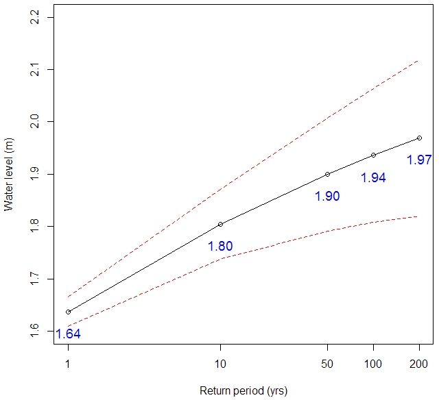
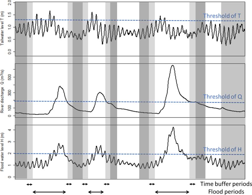
2830                                       W. Wu et al.: Estimating the probability of compound floods in estuarine regions

Figure 5. Conceptual illustration of censored continuous simulation for simulating compound flood level H in estuarine regions caused
by tailwater level in the ocean T and river discharge Q. The time periods highlighted in dark grey are low-water-level periods, while the
remaining time periods are high-water-level periods, which include flood periods and the time buffer.

The use of a time buffer accounts for the travelling time of           the entire low-water-level periods. Then the corresponding
water in the hydrodynamic model and further ensures that               flood levels are simulated using the hydrodynamic model.
the periods when flood levels H are above the suitable GPD             Thereafter, all river water level information that is not in-
threshold value (e.g. generated by combination of moderate             cluded in the high-water-level periods is sampled with re-
flood driver levels) will be fully simulated. The combination          placement from the simulated low-water-level sample based
of the flood periods and the time buffer periods is referred to        on the nearest-neighbour rule applied to both the storm tide T
as the high-water-level periods, when flood level time series          and river flow Q values. Thus, water level information for the
is fully simulated using the 2D hydrodynamic model. The                entire analysis period is obtained by combining the simulated
time periods outside these high-water-level periods are re-            water level information during the high-water-level periods
ferred to as the “low-water-level periods” and are accounted           and resampled water level information during the low-water-
for using a resampling approach described below.                       level periods.
   Since water level information below the selected thresh-               As part of the method selected for Approach 2, the
old for fitting a GPD is censored in the frequency analysis,           31 years of concurrent historical sea level and river flow
a resampling approach is used to fill in water level informa-          data are used as the basis for driving the 2D hydrodynamic
tion during the low-water-level periods, which also addresses          model of the Swan River system. A 99th percentile threshold
the challenge of not knowing a priori the exact value of the           value is selected for both flood drivers to select flood peri-
boundary condition thresholds. During the resampling pro-              ods for censored continuous simulation. This is equivalent to
cess, a random sample of the simulation period (e.g. 1000 h)           a sea water level of 1.32 m at Fremantle and a river flow of
is selected from the original flood driver time series, sub-           150 m3 s−1 at the Walyunga station. A time buffer of 12 h is
ject to values of both flood drivers being below their pre-            selected, as the average travel time of water from the upper
determined thresholds described above. In other words, only            boundary to the lower boundary of the model is under 10 h.
a fraction of the low-water-level periods is simulated, and re-        In addition, a low-water-level period sample of 1000 h is ran-
sampling with replacement is used to fill in flood data across         domly selected. Thus, this process leads to a total of 29 792 h

Hydrol. Earth Syst. Sci., 25, 2821–2841, 2021                                           https://doi.org/10.5194/hess-25-2821-2021
W. Wu et al.: Estimating the probability of compound floods in estuarine regions                                             2831

simulation time, which is approximately 10 % of the entire
31-year period under consideration. The censored simulation
                                                                              \
                                                                   Pr[X ≤ x        Y ≤ y] = GXY (x, y)
runs are carried out using a Windows server (with 2 × Xeon                                     h                   α i
E5-2698 V3 at 2.6 GHz × 256 GB RAM and 2 X K80 Tesla                                      = exp − x̃ −1/α + ỹ −1/α            (3)
GPU).
   Once the simulated water levels are obtained, the same          for x > ux , y > uy and 0 < α ≤ 1. Here, X and Y are the two
GPD-based frequency analysis described under Method 1              stochastic variables, i.e. storm tide T and river discharge Q;
is used to estimate flood probabilities at selected locations      x and y are realizations of X and Y ; G is the bivariant
based on these simulated water level data.                         distribution function of X and Y ; x̃ and ỹ are the Fréchet-
                                                                   transformed values of x and y; ux and uy are the threshold
4.3   Method 3: event-based design variable method                 values of x and y, above which function G is valid; and α is
      considering multivariate frequency analysis over             the dependence parameter, with α = 0 representing complete
      key flood-generating processes                               dependence and α = 1 representing complete independence.
                                                                   The maximum censored likelihood method can be used to es-
For Approach 3, the design variable method (DVM) (Zheng
                                                                   timate parameter α (Tawn, 1988). For the case study, the de-
et al., 2015a) is selected. The DVM was initially developed as
                                                                   pendence between flood drivers is estimated using observed
a simpler and efficient alternative to the full continuous sim-
                                                                   data of storm tide and river discharge.
ulation method, and it includes four distinct steps: (1) event
                                                                      In the third step, the hydraulic response (i.e. simulated
selection, (2) dependence model development, (3) flood sur-
                                                                   flood levels) of the selected flood events is simulated (associ-
face simulation and (4) final probability estimation. The de-
                                                                   ated with component 2 of Approach 3; see Sect. 2.4). This is
tails of these four steps are described as follows.
                                                                   often done with a 2D hydrodynamic model, which can sim-
   In the first step, compound flood events caused by different
                                                                   ulate the interaction between the two flood drivers. For this
flood drivers, such as storm tide and river discharge (i.e. com-
                                                                   study, the MIKE21 model for the Swan River is used.
binations of boundary conditions with different return peri-
                                                                      In the fourth and final step, the probability of different
ods), need to be selected for simulation. Flood levels gen-
                                                                   compound flood levels simulated in Step 3 can be derived
erated from these flood events will be interpolated to form
                                                                   based on the bivariate dependence model developed in Step 2
flood surfaces or response surfaces with different flood mag-
                                                                   using the bivariate integration method introduced by Zheng
nitudes. The DVM only requires the simulation of a limited
                                                                   et al. (2015a). More details of this integration method can be
number of flood events (often on a regular grid, e.g. 10-by-
                                                                   found in Zheng et al. (2015b).
10 flood events generated from combinations of flood drivers
with different return levels) to produce a reasonable cover of
the bivariate probability surface formed by two flood drivers
(Zheng et al., 2014, 2015a). In this study, both historical and    5     Results
synthetic flood events on an irregular grid are used to ensure
                                                                   The advantages and disadvantages of each approach are il-
flood events from drivers with a significantly longer return
                                                                   lustrated using the Swan River system case study. The re-
period than the estimated flood required are included. This is
                                                                   sults obtained from the specific implementation of each of
recommended in order to have reasonable confidence in the
                                                                   the three approaches are summarized in this section.
estimates (Zheng et al., 2014). In total, 28 flood events with
flood drivers (i.e. storm tide and river discharge) with return
                                                                   5.1    Method 1
periods of up to 1 in 250 years are selected based on the his-
torical record to produce a flood response surface with flood      The first method based on the univariate flood frequency
levels up to a return period of 1 in 100 years for the case        analysis approach is only implemented at the Barrack Street
study area. A summary of these flood events is provided in         tide gauge in the city of Perth near location Sw10 in Fig. 4,
Table S1 in the Supplement.                                        as this is the only location where relatively long records of
   In the second step, the dependence model reflecting the         observed water level data are available. The mean residual
dependence structure between the two flood drivers and their       life (MRL) plot (Fig. S1 in the Supplement) for water levels
marginal distributions needs to be developed using either ob-      observed at the Barrack Street gauge is used for threshold se-
served or simulated data (associated with component 1 of           lection. The mean excess stabilized around 1.37 m, which is
Approach 3; see Sect. 2.4). This study follows the approach        selected to be the threshold value for fitting a GPD. The es-
developed by Zheng et al. (2013, 2014, 2015a), where the bi-       timated return levels and their 95 % confidence interval (es-
variate logistic threshold excess model (Coles, 2001) is used      timated using a bootstrap method) are shown in Fig. 6. The
to quantify the dependence between the two flood drivers.          estimated flood levels range from 1.64 m for a return period
The model can be described using the following equation:           of 1 year to 1.97 m for a return period of 200 years. The con-
                                                                   fidence intervals become increasingly wide with increasing
                                                                   return period, and it is important to note that return periods

https://doi.org/10.5194/hess-25-2821-2021                                          Hydrol. Earth Syst. Sci., 25, 2821–2841, 2021
2832 W. Wu et al.: Estimating the probability of compound floods in estuarine regions
ing material. The estimated return levels at Sw1, Sw10 and
Sw12 are similar, with the 1-in-100-year return levels be-
ing 1.91, 1.89 and 1.87 m at the three locations, respectively.
The estimated 1-in-100-year flood level at location Sw19 is
much higher at 3.67 m. In addition, the 95 % confidence in-
terval for location Sw19 is much wider (higher variance)
compared to the other three locations. This is mainly be-
cause location Sw19 is flow dominated and high flood levels
are dominated by relatively few flood events in the histori-
cal record, leading to a more highly skewed distribution with
fewer data points above the threshold for flood estimation at
location Sw19 compared to the other locations.
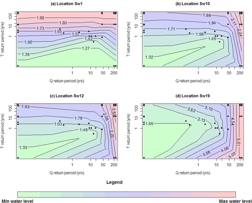
5.3 Method 3
For the design variable method (DVM), the dependence be-
Figure 6. Results of Method 1 applied to observed flood level data tween storm tide T and fluvial flood Q is first estimated using
at Barrack Street gauge near location Sw10. The black line repre- the bivariate logistic threshold excess model. The results are
sents estimated flood levels. The red dashed lines indicate the 95 % summarized in Fig. S4 for a range of time lags between T
confidence interval. and Q. The results show that the maximum dependence be-
tween storm tide T and fluvial flood Q occurs at a lag of
3 d with an α value of 0.88, indicating that the peak of flow
have been calculated based on only 22 years of historical wa- often comes 3 d after the peak of storm tide. This lag is not
ter level data. surprising given that the large catchment size generates sig-
nificant lags between rainfall events (which are more likely
5.2 Method 2 to co-occur with the storm surge peak) and the runoff to-
wards the catchment outlet. Therefore, an α value of 0.88
For the second method adopted in this case study, hourly is used for flood estimation using the DVM. This is because
flood inundation data are generated using the MIKE21 model in this method the information on the temporal dynamics of
for the entire model domain for both high-water-level periods storm surges and astronomical tides is discarded, and only
and the sampled low-water-level periods. Water level esti- the peaks of flood drivers and their joint dependence are con-
mates from the 19 marked locations (see Fig. 4) are extracted sidered, as discussed in Sect. 2.4.
from the MIKE21 model for analysis. Since the hourly wa- Flood response surfaces (i.e. flood contours) obtained for
ter levels are highly correlated, the de-clustering method de- the four selected locations are presented in Fig. 8. At loca-
scribed in Coles (2001) is used before fitting the GPD model. tion Sw1 where storm tide dominates the flood responses,
In addition, the MRL plot is used to select a suitable thresh- it can be seen that as the storm tide T becomes more ex-
old value for frequency analysis using the GPD. The MRL treme, the flood contours become horizontal and river flow Q
plots for de-clustered river level data at all 19 marked loca- has little impact on flood levels. Similar phenomena can be
tions are provided in Fig. S2. observed for location Sw19, which is flow dominated – as
In this section, results from four representative locations river flow Q becomes more extreme (especially with a re-
are selected for detailed analysis. These locations include lo- turn period of 20 years or longer), flood contours become
cation Sw1 from the tide-dominated zone, locations Sw10 vertical and storm tide T has little impact on resulting flood
and Sw12 from the joint probability zone, and location Sw19 levels. In contrast, within the joint probability zone (i.e. lo-
from the flow-dominated zone (see Fig. 4). Location Sw10 is cations Sw10 and Sw12), the flood levels are influenced by
specifically selected as it is located near the Barrack Street both flood drivers for the majority of the bivariate probability
gauge, where the only observed water level data within the surface.
river system are available (i.e. this is where the results of It can also be observed in Fig. 8 that there are some vari-
Method 1 and Method 2 can be directly compared). Based on ations in estimates of flood levels with very short return pe-
the MRL plots, a threshold value of 1.3 m is selected for lo- riods (e.g. return periods of 1 in 1 year or below), with the
cations Sw1, Sw10 and Sw12; and a threshold value of 1.4 m increase in one flood driver leading to decreased compound
is selected for location Sw19. flood levels. Careful inspection of the results shows that this
The estimated flood levels up to a return period of feature does not apply to any of the simulated data points,
200 years and their 95 % confidence intervals at these four in the sense that simulation points with larger values of the
locations are plotted in Fig. 7. The results for the remain- boundary conditions always yield larger flood levels. Rather,
ing 15 locations are provided in Figure S3 in the support- the inflection only occurs in a sparsely sampled region of
Hydrol. Earth Syst. Sci., 25, 2821–2841, 2021 https://doi.org/10.5194/hess-25-2821-2021You can also read