Future surface mass balance and surface melt in the Amundsen sector of the West Antarctic Ice Sheet - The Cryosphere
←
→
Page content transcription
If your browser does not render page correctly, please read the page content below
The Cryosphere, 15, 571–593, 2021
https://doi.org/10.5194/tc-15-571-2021
© Author(s) 2021. This work is distributed under
the Creative Commons Attribution 4.0 License.

Future surface mass balance and surface melt in the Amundsen
sector of the West Antarctic Ice Sheet
Marion Donat-Magnin1 , Nicolas C. Jourdain1 , Christoph Kittel2 , Cécile Agosta3 , Charles Amory1,2 , Hubert Gallée1 ,
Gerhard Krinner1 , and Mondher Chekki1
1 Institut
         des Géosciences de l’Environnement (IGE), Univ. Grenoble Alpes/CNRS/IRD/G-INP, Grenoble, France
2 SPHERES    research unit, Geography Department, University of Liège, 4000 Liège, Belgium
3 Laboratoire des Sciences du Climat et de l’Environnement, LSCE-IPSL, CEA-CNRS-UVSQ Université Paris-Saclay,

91198 Gif-sur-Yvette, France

Correspondence: Nicolas C. Jourdain (nicolas.jourdain@univ-grenoble-alpes.fr)

Received: 20 April 2020 – Discussion started: 1 July 2020
Revised: 3 November 2020 – Accepted: 30 November 2020 – Published: 8 February 2021

Abstract. We present projections of West Antarctic surface         face liquid water occur for higher ratios. This suggests that
mass balance (SMB) and surface melt to 2080–2100 un-               western ice shelves might remain unaffected by hydrofrac-
der the RCP8.5 scenario and based on a regional model              turing for more than a century under RCP8.5, while eastern
at 10 km resolution. Our projections are built by adding a         ice shelves have a high potential for hydrofracturing before
CMIP5 (Coupled Model Intercomparison Project Phase 5)              the end of this century.
multi-model-mean seasonal climate-change anomaly to the
present-day model boundary conditions. Using an anomaly
has the advantage to reduce CMIP5 model biases, and a
perfect-model test reveals that our approach captures most         1   Introduction
characteristics of future changes despite a 16 %–17 % under-
estimation of projected SMB and melt rates.                        In a perfectly stable climate, the Antarctic ice sheet would
   SMB over the grounded ice sheet in the sector between           have a constant mass, and the surface mass balance (SMB,
Getz and Abbot increases from 336 Gt yr−1 in 1989–2009 to          the sum of rainfall and snowfall minus sublimation, runoff,
455 Gt yr−1 in 2080–2100, which would reduce the global            and eroded snow) over the grounded ice sheet, i.e. 2000 to
sea level changing rate by 0.33 mm yr−1 . Snowfall indeed in-      2100 Gt yr−1 under the present climate (van Wessem et al.,
creases by 7.4 % ◦ C−1 to 8.9 % ◦ C−1 of near-surface warm-        2018; Agosta et al., 2019; Mottram et al., 2020), would be
ing due to increasing saturation water vapour pressure in          exactly compensated for by the ice flow across the grounding
warmer conditions, reduced sea-ice concentrations, and more        line, i.e. into the ocean. In contrast to this hypothetical stable
marine air intrusion.                                              climate, the Antarctic ice sheet has lost 2720 ± 1390 Gt of
   Ice-shelf surface melt rates increase by an order of mag-       grounded ice from 1992 to 2017, which corresponds to 7.6 ±
nitude in the 21st century mostly due to higher downward           3.9 mm of sea level rise (The IMBIE team, 2018). The main
radiation from increased humidity and to reduced albedo in         origin of the current mass loss is the acceleration of major ice
the presence of melting. There is a net production of sur-         streams (Bamber et al., 2018; The IMBIE team, 2018; Rignot
face liquid water over eastern ice shelves (Abbot, Cosgrove,       et al., 2019) mostly driven by increased oceanic melt (e.g.
and Pine Island) but not over western ice shelves (Thwaites,       Turner et al., 2017; Jenkins et al., 2018). In a warmer climate,
Crosson, Dotson, and Getz). This is explained by the evolu-        SMB may significantly increase and partly compensate for
tion of the melt-to-snowfall ratio: below a threshold of 0.60      the loss due to accelerated ice flows (e.g. Favier et al., 2017;
to 0.85 in our simulations, firn air is not entirely depleted by   Seroussi et al., 2020).
melt water, while entire depletion and net production of sur-         Recent SMB trends (1979–2000) reconstructed from firn
                                                                   cores are slightly negative, with SMB decreasing at a

Published by Copernicus Publications on behalf of the European Geosciences Union.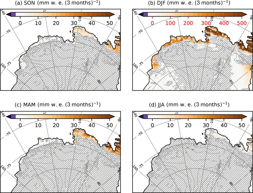
572                                                                          M. Donat-Magnin et al.: Amundsen projections

rate of −2.7 ± 3.8 Gt yr−2 for the entire ice sheet and            Trusel et al., 2015), potentially leading to higher mass loss
large differences existing between West Antarctica (−0.1 ±         through runoff and to the occurrence of melt water ponds,
1.4 Gt yr−2 ) and East Antarctica (−4.5 ± 3.5 Gt yr−2 ) (Med-      ice-shelf hydrofracturing or bending, and subsequent ice-
ley and Thomas, 2019). These trends only represent a small         shelf collapse. Based on a firn model forced by regional
fraction of the current ice-sheet imbalance (−110 Gt yr−1          atmospheric simulations constrained by global projections,
over 1992–2017), but climate models predict a significant          Kuipers Munneke et al. (2014) estimated that a few more ice
increase in Antarctic precipitation over the 21st century          shelves could experience near-complete firn air depletion by
(Krinner et al., 2007; Genthon et al., 2009; Nowicki et al.,       2100 and many more ice shelves by 2200 in East and West
2020). Under the A1B or RCP8.5 scenarios to 2100, sim-             Antarctica under the strongest emission scenario. Using re-
ulated Antarctic SMB increases by 13 % to 25 % depend-             gional atmospheric simulations and global projections with
ing on the climate model (Agosta et al., 2013; Ligtenberg          bias corrections, Trusel et al. (2015) reported that large frac-
et al., 2013; Lenaerts et al., 2016; Palerme et al., 2017).        tions of East and West Antarctic ice shelves could experience
These changes are strongly related to temperatures (Frieler        melt rates greater than the pre-collapse value of Larsen B by
et al., 2015) with an SMB sensitivity of 5 %–7 % per degree        the end of the 21st century under the warmest scenario.
of near-surface warming (Krinner et al., 2008; Ligtenberg             Computing projections of future SMB and surface melt
et al., 2013; Agosta et al., 2013; Palerme et al., 2017). In a     rates remains challenging because of the strong natural vari-
warmer climate, the saturation water vapour pressure indeed        ability at regional scales (Lenaerts et al., 2016; Donat-
increases (Clapeyron, 1834; Clausius, 1850), and more hu-          Magnin et al., 2020b), biases in global climate models
midity can be transported over the ocean and made available        (GCMs) (Bracegirdle et al., 2013; Swart and Fyfe, 2012),
for Antarctic precipitation.                                       and GCM resolutions that are too coarse to resolve the oro-
   Runoff into the ocean is a negative contribution to SMB. It     graphic processes in the relatively steep coastal area (Krinner
is produced if surface melt and/or rain rates are high enough      et al., 2008; Lenaerts et al., 2012; Agosta et al., 2013). Most
to (i) bring the temperature of underlying snow and firn           models that participated in the Climate Model Intercompar-
layers to the freezing point and (ii) percolate and saturate       ison Project Phase 5 (CMIP5; Taylor et al., 2012) overesti-
the pore space in the snow and firn layers, which is some-         mated the present-day Antarctic precipitation by more than
times referred to as firn air depletion (Pfeffer et al., 1991;     100 % in some cases (Palerme et al., 2017). These models
Kuipers Munneke et al., 2014; Alley et al., 2018). Currently,      also had a generally poor representation of the snow-pack
runoff is at least 3 orders of magnitude smaller than precip-      energy balance, which is why future melt-rate estimates have
itation for the entire Antarctic ice sheet (van Wessem et al.,     often been derived from simulated air temperatures rather
2018; Agosta et al., 2019). Surface melt and/or rainfall be-       than being directly provided by the models (Davies et al.,
yond the pore space saturation do not necessarily lead to          2014; Trusel et al., 2015), and most limitations remain rele-
runoff. Liquid water in excess can alternatively be trans-         vant in the CMIP6 models (Mudryk et al., 2020). Recent ver-
ported horizontally on the ice shelf and/or form ponds. In         sions of regional climate models (RCMs) with a comprehen-
some circumstances, these processes can trigger ice-shelf          sive representation of polar processes are now able to sim-
collapse through hydrofracturing or ice-shelf bending (e.g.        ulate melt rates in reasonable agreement with observational
Bell et al., 2018; Robel and Banwell, 2019; Lai et al., 2020)      estimates when they are driven by reanalyses (van Wessem
with important consequences for the ice-sheet dynamics (Sun        et al., 2018; Lenaerts et al., 2018; Datta et al., 2019; Donat-
et al., 2020).                                                     Magnin et al., 2020b). Using this kind of RCM to down-
   Surface melt only occurs to a significant extent over the       scale simulations from GCMs can significantly reduce sur-
peninsula (Scambos et al., 2009; Trusel et al., 2013) and spo-     face biases (Fettweis et al., 2013). However, this approach is
radically in other regions like the Amundsen Sea (Nicolas          not sufficient to remove the large-scale biases inherited from
et al., 2017; Donat-Magnin et al., 2020b) and Ross Sea (Bell       GCMs, and bias corrections of the GCM solution (Trusel
et al., 2017; Wille et al., 2019) sectors. Over most ice shelves   et al., 2015; Beaumet et al., 2019a) may be needed prior to
in Antarctica, current melt and rainfall rates are nonethe-        RCM downscaling. In this paper, we build SMB and surface
less low compared to snowfall rates, and there is no signif-       melt projections for the end of the 21st century by forcing
icant firn air depletion (Kuipers Munneke et al., 2014). In        an RCM with the 3-dimensional climate-change anomalies
such circumstances, the resulting liquid water is buried in        from a CMIP5 RCP8.5 multi-model mean with the aim of
the snow and likely refreezes. An exception is the eastern         removing a part of the CMIP model biases (see Sect. 2).
side of the Antarctic Peninsula that experienced melt water           We focus on the Amundsen Sea sector, where potential
ponds and the resulting collapse of the Larsen B ice shelf         future melt-induced hydrofracturing and associated loss of
(Vaughan et al., 2003; van den Broeke, 2005; Scambos et al.,       ice-shelf buttressing could have strong effects on the stabil-
2009) and where simulations suggest nearly depleted firn air       ity of the West Antarctic Ice Sheet and therefore on sea level
(Kuipers Munneke et al., 2014).                                    rise (Pattyn et al., 2019). Currently, the Amundsen sector ac-
   In a warmer climate, surface melt increases exponentially       counts for 60 % of the total Antarctic mass loss (Rignot et al.,
with surface air temperature (Kuipers Munneke et al., 2014;        2019). While oceanic melting is currently the dominant pro-

The Cryosphere, 15, 571–593, 2021                                                       https://doi.org/10.5194/tc-15-571-2021
M. Donat-Magnin et al.: Amundsen projections                                                                                   573

cess causing mass loss (Thoma et al., 2008; Turner et al.,          water retention of 10 % of the porosity in each successive
2017; Jenkins, 2016; Jenkins et al., 2018), surface air temper-     layer. The firn layers are fully permeable until they reach
ature is expected to increase (Bracegirdle et al., 2008), and       a close-off density of 830 kg m−3 . To account for possible
whether the ice shelves of the Amundsen sectors will respond        cracks in ice lenses and moulins, the part of available wa-
with the same hydrofracturing mechanism as in the Antarctic         ter that is transmitted downward to the next layer decreases
Peninsula remains an open question. Contrasting behaviours          as a linear function of firn density, from 100 % transmitted
were indeed projected for individual ice shelves in previ-          at the close-off density to zero at 900 kg m−3 and denser. If
ous studies at relatively coarse resolutions (Kuipers Munneke       the liquid water is not able to percolate further down, then it
et al., 2014; Trusel et al., 2015). In the following, we describe   fills the entire porosity space of surface layers, and the ex-
our general methodology (Sect. 2), then we describe future          cess is removed from the simulated snow/firn because there
projections in Sect. 3 with a particular focus on SMB over          is no representation of ponds or horizontal routing of liquid
the grounded ice sheet (relevant for sea level) and melting         water in our version of MAR. In this paper, we refer to the
over the ice shelves (relevant for hydrofracturing). We then        formation rate of liquid water in excess as “net production
propose an extrapolation of our results to other scenarios and      of surface liquid water”, and we use it as an indicator of po-
time horizons, and we thoroughly discuss the impact of mod-         tential ice-shelf collapse. Liquid water in excess can indeed
elling and methodological biases in our projections (Sect. 4).      accumulate in ponds or flow into crevasses (potentially in-
                                                                    ducing hydrofracturing) or into the ocean (potentially induc-
                                                                    ing ice-shelf bending). It is important to keep in mind that
2     Method                                                        this is only a potential for collapse because the liquid wa-
                                                                    ter can flow into the ocean in some cases (thereby protecting
2.1    Regional atmosphere and firn model                           the ice shelf from hydrofracturing; Bell et al., 2017) and be-
                                                                    cause there are mechanical conditions for hydrofracturing to
Our projections of the West Antarctic surface climate for           develop (Lai et al., 2020).
the end of the 21st century are based on version 3.9.3 of
the MAR regional atmospheric model (Gallée and Schayes,             2.2   Present-day and future forcing
1994; Agosta et al., 2019). Our regional configuration is cen-
tred on the Amundsen Sea sector, covers 2800×2400 km, and           The simulation representative of the present climate is the
was developed by Donat-Magnin et al. (2020b). The horizon-          one described in Donat-Magnin et al. (2020b). It is forced
tal resolution is 10 km, and we use 24 vertical sigma levels        laterally (pressure, wind, temperature, specific humidity), at
located from approximately 1 m above the ground to 0.1 hPa.         the top four levels (temperature, wind), and at the surface
The topography is derived from BEDMAP2 (Fretwell et al.,            (sea-ice concentration, sea surface temperature, SST) by 6-
2013), and the drainage basins used for averages are those          hourly outputs of the ERA-Interim reanalysis (Dee et al.,
defined by Mouginot et al. (2017).                                  2011), which has a good representation of the Antarctic cli-
    The radiative scheme and cloud properties are the same          mate (Bromwich et al., 2011; Huai et al., 2019). A thorough
as in Datta et al. (2019), and the surface scheme, includ-          evaluation of the present-day simulation with respect to in
ing snow density and roughness, are the same as in Agosta           situ and satellite observational products is provided in Donat-
et al. (2019). The atmosphere is coupled to the SISVAT sur-         Magnin et al. (2020b) and indicates a good fidelity of the sim-
face scheme (Soil Ice Snow Vegetation Atmosphere Trans-             ulated surface mass balance and melt rates. Here we further
fer; Gallée and Duynkerke, 1997; Gallée et al., 2001), which        show that simulated present SMB values over the grounded
here is a 30-layer snow and firn model representing the first       parts of Pine Island and Thwaites (Table 1) are within the ob-
20 m with refined resolution at the surface. It includes prog-      servational range of uncertainty estimated by Medley et al.
nostic equations for temperature, mass, water content, and          (2014) after correction to account for different basin areas
snow properties (dendricity, sphericity, and grain size). SIS-      (their Table 3). In the present paper, we do not describe or
VAT and the atmosphere are coupled through exchanges of             discuss features located eastward of 75◦ W (e.g. George VI
mass fluxes, as well as radiative and turbulent heat fluxes.        Ice Shelf) and southward of 78◦ S (e.g. Ross and Ronne ice
    Surface albedo depends on the evolving snow properties          shelves) as these locations are considered too close to the re-
and on the solar zenithal angle (Tedesco et al., 2016). As          laxation zone of the model domain where lateral boundary
in Agosta et al. (2019), the density of fresh snow increases        conditions are prescribed.
with wind speed (+6.84 kg m−3 (m s−1 )−1 ) and temperature             For the future, we calculate the climate-change absolute
(+0.48 kg m−3 ◦ C−1 ) at the time of snow deposit, and our          anomaly from a CMIP5 multi-model mean (MMM), and we
set-up does not include drifting snow, which is not con-            add it to the 6-hourly ERA-Interim variables used to drive
sidered as a strong limitation for this sector of Antarctica        MAR, i.e. sea surface temperature (SST), sea-ice concen-
(Lenaerts et al., 2012), although this remains a poorly quan-       tration (SIC), and 3-dimensional wind velocity, air temper-
tified process. In the case of surface melt or rainfall, liquid     ature, and specific humidity. Considering all these anoma-
water percolates downward into the next firn layers with a          lies together allows us to keep the consistency of linear re-

https://doi.org/10.5194/tc-15-571-2021                                                      The Cryosphere, 15, 571–593, 2021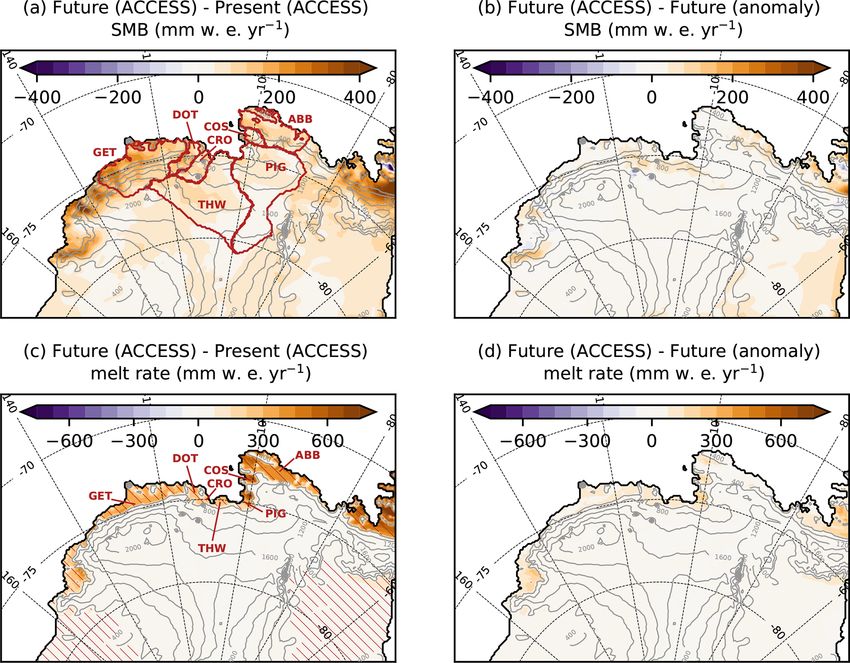
574                                                                                   M. Donat-Magnin et al.: Amundsen projections

Table 1. (a) SMB and its components over the grounded part of individual glacial drainage basins for the present day (regular) and future
(bold). The results are here provided in gigatons per year (Gt yr−1 ), i.e. integrated over the drainage basins (areas indicated in b), to be
directly convertible into a rate of sea level rise. SMB is the sum of snowfall and rainfall minus sublimation and runoff. Here we assume that
the net production of surface liquid water is equivalent to runoff because of the significant slopes over the coastal grounded ice sheet. (c) The
relative increase in snowfall per degree of air warming at 2 m above ground level (see Eq. 1).

           (a) SMB component (Gt yr−1 )               Abbot    Cosgrove      Pine Island    Thwaites    Crosson     Dotson      Getz
              SMB                                      36.3          7.1           80.1         95.9        20.6       16.9     79.3
                                                       50.8         10.0          110.2        129.1        28.4       22.9    103.5
              Snowfall                                 37.0          7.3           82.0         95.6        21.0       17.3     81.0
                                                       50.5         10.0          111.3        127.7        28.6       23.2    104.5
              Rainfall                                  0.1           0.0            0.1          0.0         0.1        0.0      0.0
                                                        0.7           0.1            0.3          0.1         0.2        0.1      0.2
              Sublimation                               0.7           0.2            2.0        −0.2          0.5        0.4      1.7
                                                        0.4           0.1            1.1        −1.3          0.4        0.3      1.2
              Runoff                                    0.0           0.0            0.0          0.0         0.0        0.0      0.0
                                                        0.1           0.0            0.3          0.0         0.0        0.0      0.0
           (b) Area (103 km2 )                         30.0           8.8         186.3        192.4        23.5       16.2.     90.0
           (c) Snowfall rel. sensitivity (% ◦ C−1 )   +8.5          +8.4           +8.1         +7.8        +8.9       +8.6     +7.4

lationships, such as the geostrophic and thermal wind bal-                  zero SIC unchanged) does not conserve the applied CMIP5
ances, although it does not necessarily conserve non-linear                 anomaly. To circumvent this issue, we apply the anomaly
relationships. This type of method was previously referred                  through 20 iterations: we start applying the CMIP5-MMM
to as “anomaly nesting” (Misra and Kanamitsu, 2004) or                      anomaly to the days and locations with SIC greater than zero
“pseudo global warming” (e.g. Kimura and Kitoh, 2007),                      (for negative anomaly) and smaller than 100 % (for positive
although this term was often used for more simple temper-                   anomaly), and after each iteration, we calculate the resid-
ature and humidity perturbation methods (e.g. Schär et al.,                 ual SIC that would be needed to reach the original CMIP5-
1996). The MMM anomaly is defined as the mean differ-                       MMM SIC anomaly, and we add it to the applied climatolog-
ence between 1989–2009 and 2080–2100 under the RCP8.5                       ical anomaly. The effect of this sea-ice anomaly correction
emission scenario for an ensemble of 33 CMIP5 models (see                   is briefly described in Sect. 4. Alternative sea-ice correction
Appendix A). The anomaly is calculated separately for each                  methods were evaluated by Beaumet et al. (2019b), but here
calendar month, meaning that we apply an anomaly that in-                   we prefer to stay as close as possible to the simple anomaly
cludes a seasonal cycle. Monthly anomalies are linearly in-                 method used for the other variables.
terpolated to avoid discontinuity of 6-hourly boundary con-                    As discussed by Knutti et al. (2010), the MMM is often
ditions. In the future simulation, we do not modify green-                  considered as the “best” estimate for future climate because
house gas concentrations in our regional domain, which is                   individual model biases are partly cancelled in the MMM,
expected to have a minor effect because the dominant effect                 although an equal weight for all the models does not ac-
of global increase in greenhouse gas concentrations on our                  count for the fact that models are not independent from each
regional simulations comes from changes in sea surface and                  other because of the same operating centres, common his-
sea-ice forcing, as well as through increased humidity and                  tory, shared physical parameterisations, and numerical meth-
temperature at the lateral boundaries (Krinner et al., 2014;                ods (Knutti et al., 2017; Herger et al., 2018). Given that the
Bull et al., 2020).                                                         CMIP model biases are largely stationary even under strong
   Adding an anomaly is relatively simple but requires a spe-               climate changes (Krinner and Flanner, 2018), our method is
cific calculation for two variables. First, specific humidity is            also expected to remove a part of the biases in individual
set to zero in rare cases when applying the CMIP5 anomaly                   model projections. This method has previously been used in
would produce unphysical negative values. Second, sea-ice                   various regional studies (e.g. Sato et al., 2007; Knutson et al.,
concentration (SIC) anomalies are applied through an itera-                 2008; Michaelis et al., 2017; Dutheil et al., 2019) but, to our
tive process, which is needed because some locations have                   knowledge, never in Antarctica. Krinner et al. (2008, 2014)
non-zero SIC on some days and zero SIC on other days. As                    and Beaumet et al. (2019a) used anomalies in global simu-
negative SIC values are unphysical, applying a negative cli-                lations with a stretched grid over Antarctica, but this only
matological SIC anomaly to all days (but keeping days with                  involved anomalies in sea surface conditions.

The Cryosphere, 15, 571–593, 2021                                                                 https://doi.org/10.5194/tc-15-571-2021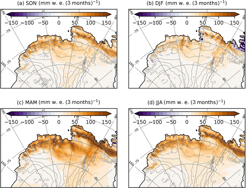
M. Donat-Magnin et al.: Amundsen projections 575
All the simulation years are run in parallel with a 12- from 336 Gt yr−1 presently to 455 Gt yr−1 by the end of the
year spin-up for each simulated year, which is sufficient to 21st century (Table 1). As previously reported by Ligten-
obtain a steady net production of surface liquid water in berg et al. (2013), increasing snowfall explains most of the
the future simulation over all ice shelves except Abbot (see SMB changes. Projected sublimation slightly decreases in all
Sect. 4). When not stated otherwise, the present-day period basins, while rainfall slightly increases, but both components
represents 1988–2017. The future period corresponds to the remain 2 orders of magnitude smaller than snowfall. Runoff
1988–2017 period to which was added the CMIP5-MMM is projected to remain negligible over the grounded ice sheet
anomaly (2080–2100 minus 1989–2009) and therefore repre- in this sector.
sents something like 2079–2108 (with the inter-annual vari- We now briefly analyse possible causes for increased SMB
ability of 1988–2017). While our CMIP5-MMM anomaly in a warmer climate. In the following, the relative increase A
is only based on 21 years, we decided to run our regional in a variable V (saturation water vapour pressure or snow-
simulations over 30 years, which provides more statistical fall) per degrees of warming is calculated by integrating the
significance given that surface melt rates and SMB exhibit following:
high inter-annual variability in this region (Scott et al., 2019;
Donat-Magnin et al., 2020b). Retrospectively, it would have A = 1 dV
V dT
been better to use the same 30-year time window for CMIP5 1
V2
, (1)
and for our MAR simulations.
= T2 −T1 ln V1
We now briefly describe the CMIP5-MMM anomalies ap-
plied to ERA-Interim. The troposphere is warmed relatively which has the advantage to give A values that are relatively
uniformly from the surface to ∼ 300 hPa (Fig. 1a). There independent of the chosen (T2 − T1 ) temperature interval
is a clear seasonal cycle in the low-tropospheric anomalies given the approximate exponential relationship expected for
with stronger warming in winter than in summer. This is re- the variables under consideration.
lated to stronger changes in winter sea-ice cover compared to The saturation water vapour pressure increases with air
summer (solid lines in Fig. 2) because present-day summers temperature at a rate of 7.1 ± 0.1 % ◦ C−1 in the 0–10 ◦ C
are already relatively sea-ice free, and, as such, sea-ice cover range (Clausius–Clapeyron relation). In our simulations,
cannot decrease much further. As expected from the radiative near-surface warming reaches 3.4 to 3.7 ◦ C for the various
effects of greenhouse gases, the stratosphere tends to cool in basins, which is very close to the RCP8.5 MMM global
response to the increased anthropogenic emissions of green- warming value (Collins et al., 2013). The corresponding in-
house gases (e.g. Seidel et al., 2011). There is also a clear crease in snowfall over the grounded ice sheet represents
seasonal cycle in the lower stratosphere (∼ 100 hPa) with fu- +7.4 to +8.9 % ◦ C−1 (Table 1c), which is higher than the
ture warming in spring and summer and cooling in the other theoretical Clausius–Clapeyron rate. This indicates that other
seasons which is related to seasonal effects of ozone recov- factors may contribute to increasing snowfall in the Amund-
ery (Perlwitz et al., 2008). Specific humidity increases as the sen sector.
troposphere warms (Fig. 1b), as expected from the Clausius– To further understand the mechanism for increased snow-
Clapeyron relation. fall, we now consider projections for the four seasons sep-
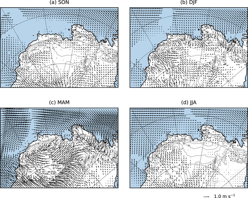
arately (Fig. 4). The strongest increase in SMB occurs in
MAM (March, April, May; followed by JJA, June, July,
3 Results August), which corresponds to the season with the largest
changes in sea-ice concentrations in the vicinity of the ice-
In this section, we present SMB and surface melt projections sheet margin (see dashed lines in Fig. 2). While Clausius–
derived from ERA-Interim and the CMIP5-MMM-RCP8.5 Clapeyron refers to the maximum saturation water vapour
anomaly. We simply refer to the corresponding simulations pressure, we suggest that decreasing coastal sea-ice cover
as “present” and “future” in the following. We also inves- makes surface air masses closer to their saturation level,
tigate the causes for these changes, and we discuss conse- as previously suggested by Gallée (1996) and Kittel et al.
quences for potential ice-shelf hydrofracturing and sea level (2018). This mechanism is also consistent with the modelling
rise. results of Wang et al. (2020) who find that precipitation over
the coastal Amundsen region mostly comes from evaporation
3.1 Grounded ice-sheet SMB occurring all the way from the Tropical Pacific to the Amund-
sen Sea. Another possible contributor to increased snowfall
The future SMB is increased by 30 % to 40 %, keeping a very is the changing low-tropospheric circulation which shows a
similar pattern to the present day (Fig. 3a, b), i.e. mostly con- cyclonic anomaly in MAM favouring humidity transport to-
trolled by the steep slopes and local topographic features near wards the ice sheet (Fig. 5). As warming at the height where
the ice-sheet margin. Considering the grounded part (which precipitation is formed is relevant for Clausius–Clapeyron, a
matters for sea level rise) of all the drainage basins from Getz stronger warming farther above the surface than in its vicin-
to Abbot (boundaries indicated in Fig. 3a), SMB increases ity could also contribute in explaining this stronger sensitiv-
https://doi.org/10.5194/tc-15-571-2021 The Cryosphere, 15, 571–593, 2021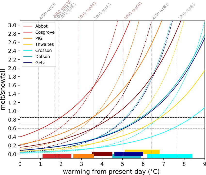
576                                                                           M. Donat-Magnin et al.: Amundsen projections

Figure 1. (a) Temperature and (b) specific humidity vertical profiles of the CMIP5-MMM anomaly (2080–2100 minus 1989–2009) that is
added to ERA-Interim, here spatially averaged over West Antarctica (60–85◦ S, 170–40◦ W).

                                                                    crease from typically a week per year to 1–2 months per year
                                                                    (Table 2). As previously noticed by Kuipers Munneke et al.
                                                                    (2014) and Trusel et al. (2015), we find an exponential de-
                                                                    pendency of melt rates to 2 m air temperatures (not shown)
                                                                    with a much stronger dependency on temperature than SMB
                                                                    (Clausius–Clapeyron). In terms of seasonality, future melt
                                                                    rates are strongly increased in summer (DJF) over all the ice
                                                                    shelves, while Abbot, Cosgrove, and Pine Island also experi-
                                                                    ence significantly more melting in fall and spring (Fig. 6).
                                                                       Rainfall is also projected to increase (Table 2) but repre-
                                                                    sents a relatively small fraction of surface melt (less than
                                                                    15 % for all the ice shelves). Future surface melt and rain-
                                                                    fall entirely refreeze in the firn for all the ice shelves from
Figure 2. Mean seasonal cycle of sea-ice concentration over the     Getz to Thwaites, which leads to zero net surface liquid wa-
oceanic part of the MAR domain (solid) and southward of 70◦ S       ter production in the future. In contrast, Abbot, Cosgrove,
(dashed) for the present-day (blue) and future (dark-red) simula-   and Pine Island have a positive net surface liquid water pro-
tions.                                                              duction, although most surface melt and rainfall still refreeze
                                                                    in the firn.
                                                                       The contrast between western (Getz to Thwaites) and east-
ity, although Fig. 1a suggests slightly stronger near-surface
                                                                    ern (Pine Island to Abbot) ice shelves can be explained by
warming.
                                                                    variations in the melt-to-snowfall ratio, which we now ex-
3.2   Ice-shelf surface liquid water budget                         plain from simple considerations. As rainfall remains signif-
                                                                    icantly weaker than melt rates, we neglect it in the following
We have shown that runoff plays no significant role in the          discussion, but more details on the theoretical role of rain-
simulated SMB over the grounded ice sheet and therefore             fall are provided in Appendix B. First of all, if surface melt
on sea level projections. However, surface melt, rainfall, and      water percolates into snow layers that are below the freez-
subsequent net production of surface liquid water may lead          ing point, it partly refreezes, which releases latent heat and
to ponding over ice shelves and trigger hydrofracturing. In         warms the snow layers. Therefore, the melt-to-snowfall ratio
this section, we therefore focus on liquid water budget pro-        must typically exceed a few hundredths to bring the snow to
jections over the seven major ice shelves from Getz to Abbot.       0 ◦ C and allow the existence of liquid water in snow. To have
In this paper, we do not investigate supra-glacial hydrology        a net production of surface liquid water, melt rates also need
and hydrofracture mechanics in detail; we simply consider           to be sufficiently high to significantly deplete air in snow.
the presence of the net production of surface liquid water as       Based on a simple model, Pfeffer et al. (1991) estimated that
an indicator of potential ice-shelf collapse (i.e. a necessary      surface melt would lead to snow-air depletion for melt-to-
but not sufficient condition).                                      snowfall ratios greater than approximately 0.7, considering
   Surface melt rates averaged over the major individual ice        fresh-snow and close-off densities of 300 and 830 kg m−3 ,
shelves from Getz to Abbot are projected to increase by 1           respectively (see Appendix B). This shows that in the pres-
order of magnitude, and melt occurrence is projected to in-         ence of relatively fresh snow, large melt-to-snowfall ratios

The Cryosphere, 15, 571–593, 2021                                                       https://doi.org/10.5194/tc-15-571-2021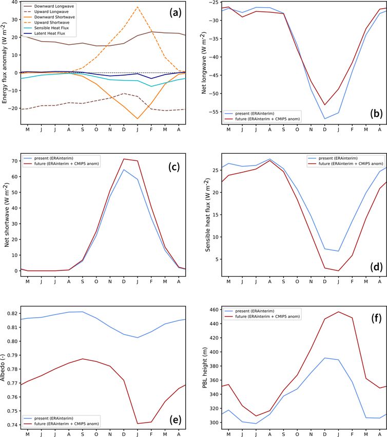
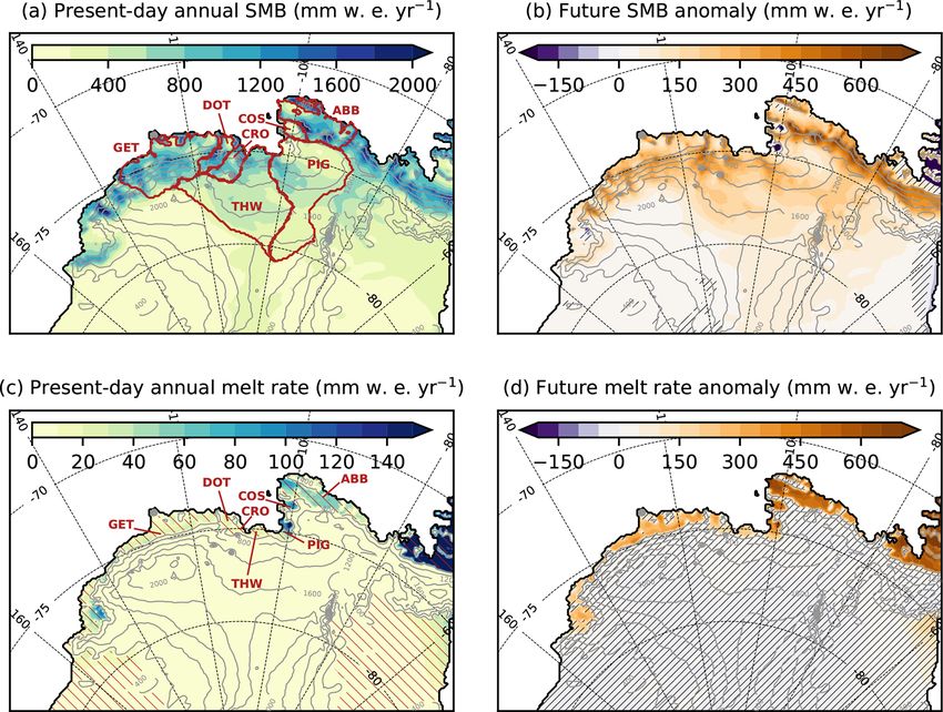
M. Donat-Magnin et al.: Amundsen projections                                                                                                   577

Figure 3. (a) Present-day annual mean SMB and (b) annual mean SMB anomaly (future minus present). (c) Present-day annual mean melt
rate and (d) annual mean melt-rate anomaly (future minus present). The dark red contours in (a) indicate individual glacial drainage basins:
Getz (GET), Dotson (DOT), Crosson (CRO), Thwaites (THW), Pine Island Glacier (PIG), Cosgrove (COS), and Abbot (ABB). Red hatching
in (c) indicates ice shelves. Black narrow hatching in panels (b, d) indicate areas where the difference is not statistically significant (t test on
annual means with a p value of 0.05). The ice-sheet topography is shown in grey (contours every 400 m).

are needed to have a net production of surface liquid wa-                   sence of net production of surface liquid water in a warmer
ter because large melt rates are needed to fill the porosity                climate. Concerning Pine Island, it should be noted that high
brought by large snowfall. In contrast, small quantities of                 melt rates are concentrated on its north-eastern flank (Figs. 3,
melt or rain water are buried in large snowfall and likely re-              6), so potential hydrofracturing may be limited to that part,
freeze.                                                                     which is not the most important in terms of ice-sheet dynam-
   Going back to our simulations, we note the importance                    ics and instability (e.g. Favier et al., 2014).
of the melt-to-snowfall ratio for the net production of sur-                   We now briefly analyse the causes for increased melting
face liquid water simulated by MAR over the ice shelves,                    in a warmer climate. All along the future melting season,
with episodic production for annual melt-to-snowfall ratios                 less energy is lost by the ice-shelf surface through net long-
as low as 0.25 and a highly probable production for annual                  wave radiation (Fig. 8b), which is a consequence of higher
melt-to-snowfall ratios greater than ∼ 0.85 (Fig. 7). The ra-               downward longwave radiation, as expected in the presence
tio allowing the production of surface liquid water exhibits                of higher specific humidity and only partly compensated for
some variability due to varying snow characteristics and a                  by higher upward longwave radiation emitted by a warmer
more complex firn model than in Pfeffer et al. (1991), but on               snow surface in the future (Fig. 8a, b). In the future, more en-
average, surface liquid water becomes more likely than not                  ergy is also received by the snow surface through shortwave
for melt-to-snowfall ratios greater than 0.85.                              radiative fluxes over the melting season (Fig. 8c), which is
   The existence of such a threshold explains the variations                explained by a melt–albedo feedback, i.e. a decreased ice-
in liquid water production across the ice shelves (Table 2b);               shelf albedo as a result of more melting (Fig. 8e). These
Abbot, Cosgrove, and Pine Island have relatively high future                changes are partly compensated for by less shortwave radi-
melt rates (∼ 500 mm w.e. yr−1 ), but Abbot receives much                   ation received by the snow surface (negative anomaly of the
higher snowfall, which explains that surface melt produces                  downward component in Fig. 8a), which is explained by a
less surface liquid water than over Cosgrove and Pine Is-                   moderate increase in summer cloudiness (not shown) in the
land; the four other ice shelves experience both relatively                 future. Changes in sensible and latent heat fluxes are less im-
high snowfall and weak melt rates, which explains the ab-                   portant than changes in radiative forcing, but they compen-

https://doi.org/10.5194/tc-15-571-2021                                                                  The Cryosphere, 15, 571–593, 2021
578                                                                                 M. Donat-Magnin et al.: Amundsen projections

Figure 4. Changes in mean seasonal SMB (future minus present). Black narrow hatching indicates areas where the difference is not statisti-
cally significant (t test on 3-month means with a p value of 0.05). The ice-sheet topography is shown in grey (contours every 400 m).

Table 2. (a) Components of the surface liquid water budget and snowfall over individual ice shelves for the present day (regular) and future
(bold). “Net liquid” is the sum of melting plus rainfall minus refreezing minus the liquid water retained in the firn without refreezing (zero
in our case; not shown). Here we present average values in millimetre water equivalent per year (mm w.e. yr−1 , i.e. kg m−2 yr−1 ), which is
thought to be more meaningful than integrated values in terms of hydrofracture potential. (b) The melt-to-snowfall ratio. (c) The number of
rain days (threshold of 1 mm w.e. day−1 ) and the number of melt days per year (threshold of 3 mm w.e. day−1 as in Donat-Magnin et al.,
2020b).

             (a) Component (mm w.e. yr−1 )        Abbot     Cosgrove     Pine Island    Thwaites     Crosson    Dotson     Getz
                 Melting                              54           80             79          26          17         21      22
                                                     577          588            455         244         183        292     333
                 Refreezing                           60           83             85          29          20         24      25
                                                     613          462            372         268         201        310     348
                 Rainfall                              6            3              6            3          3          3       2
                                                      77           27             33           25         18         18      17
                 Net liquid                            0            0              0            0           0         0       0
                                                      40          153            116            0           0         0       1
                 Snowfall                            790          290            407         809        1055        669     786
                                                     943          372            521         989        1339        830     978
             (b) Melt / snowfall                    0.07         0.28           0.19         0.03       0.02       0.03    0.03
                                                    0.61         1.58           0.87         0.25       0.13       0.35    0.34
             (c) Number of rain days per year        1.0          0.6            1.0          0.5        0.4        0.3     0.4
                                                    14.0          5.7            5.8          4.2        3.1        2.9     3.1
                 Number of melt days per year        7.8         10.7           10.2          3.5        2.3        2.9     3.1
                                                    65.3         63.2           46.6         31.0       25.3       38.0    42.7

The Cryosphere, 15, 571–593, 2021                                                               https://doi.org/10.5194/tc-15-571-2021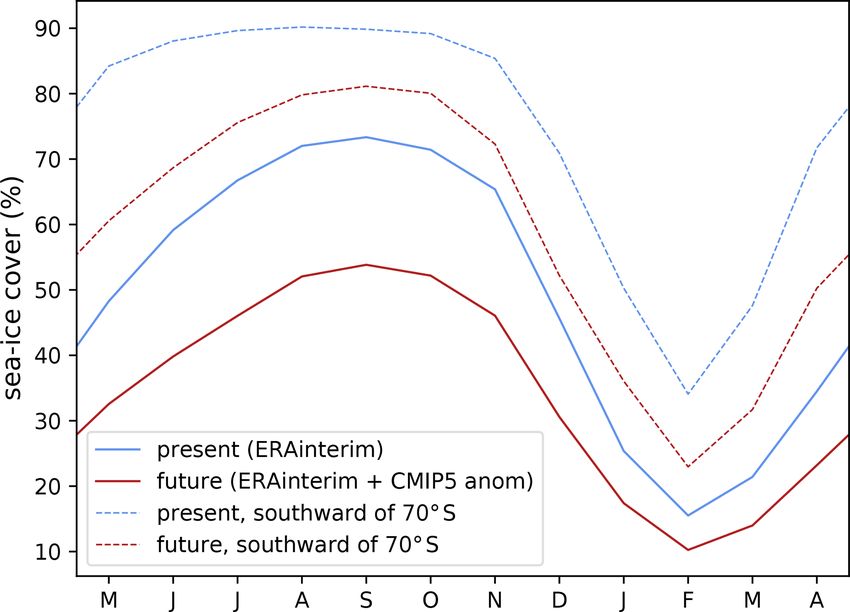
M. Donat-Magnin et al.: Amundsen projections                                                                                             579

Figure 5. Changes in mean seasonal 10 m winds (future minus present). Vectors are not displayed at locations where the change in at least
one of the wind components is not statistically significant (t test on 3-month means with a p value of 0.05). The open ocean is in light blue,
and the ice-sheet topography is shown in grey (contours every 400 m).

sate for a part of the increased net longwave and shortwave              4.1    Extrapolation to other climate perturbations
radiation (Fig. 8a, d). This may be related to a thicker plane-
tary boundary layer in the future (Fig. 8f), i.e. reduced near-          While CMIP5-MMM-RCP8.5 at the end of the 21st century
surface temperature and humidity vertical gradients similar              is meaningful, it is also interesting to estimate the likeli-
to the difference between summer and winter (Fig. 8d, f).                hood of net production of surface liquid water over the ice
                                                                         shelves further in the future or following alternative emis-
                                                                         sion scenarios. To do so, we evaluate the melt-to-snowfall
4   Discussion
                                                                         ratio for a given additional warming or cooling, assuming
We first discuss the possibility to extrapolate our results to           that snowfall (SNF) and melt rates (MLTs) evolve follow-
other climate perturbations. Then, we discuss some limita-               ing simple relationships with temperature. Such relationships
tions of our modelling and methodological approaches and                 can be obtained from the literature. The snowfall dependency
their impacts on our projections.                                        to temperature can be obtained by the Magnus empirical fit of
                                                                         the Clausius–Clapeyron relationship (Koutsoyiannis, 2012),
                                                                         here further simplified by linearising the term of the expo-
                                                                         nential around 0 ◦ C. The melt rate also has an exponential
                                                                         dependency to near-surface temperature, with an empirical
                                                                         expression derived by Trusel et al. (2015) from a numerical
                                                                         model applied to the entire Antarctic ice sheet. For a given

https://doi.org/10.5194/tc-15-571-2021                                                              The Cryosphere, 15, 571–593, 2021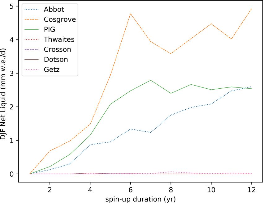
580 M. Donat-Magnin et al.: Amundsen projections
Figure 6. Changes in seasonal mean melt rates (future minus present). The colour-bar labels in panel (b) are shown in red to emphasise
the different range compared to the other panels. Black hatching indicates areas where the difference is not statistically significant (t test on
3-month means with a p value of 0.05). The ice-sheet topography is shown in grey (contours every 400 m).
ice shelf (is), this yields the following:
17.625(1T −1Tp )
SNFis (1T ) = SNFis,p exp 243.04
= SNFis,p exp 0.072(1T − 1Tp )
MLTis (1T ) = MLTis, p exp 0.456(1T − 1Tp ) , (2)
MLTis (1T )
Ris (1T ) =
SNFis (1T )
= Ris, p exp 0.384(1T − 1Tp )
where 1T represents warming with respect to the present
day (1989–2009) and 1Tp is the CMIP5-MMM-RCP8.5
warming analysed in this study (2080–2100 minus 1989–
2009). The two first lines of Eq. (2) are obtained by us-
ing the simulated future values on individual ice shelves at
Figure 7. Net production of surface liquid water vs. melt-to- 1T = 1Tp , i.e. SNFis, p and MLTis, p . The third line gives
snowfall ratio in the future simulation (calculated from climatologi- the melt-to-snowfall ratio of a given ice shelf (Ris ).
cal means). Each circle represents the climatological annual mean at While the expressions in Eq. (2) have the advantage to be
a grid point within the seven glacial drainage basins. The solid curve theoretically valid for general Antarctic conditions, local fits
is a Gaussian kernel density estimate with a standard deviation of based on our simulations are also meaningful. Another ex-
0.1 for the melt-to-snowfall ratio. The vertical dashed lines indicate
pression can be derived assuming the same exponential form
the limit above which more than 10 % and 50 % of the points expe-
rience a net production greater than 1 mm w.e. yr−1 .
as Eq. (2) but with a coefficient in the exponential calculated
as the average of the seven values calculated for individual
ice shelves:
Ris = Ris, p exp 0.577(1T − 1Tp ) . (3)
The Cryosphere, 15, 571–593, 2021 https://doi.org/10.5194/tc-15-571-2021M. Donat-Magnin et al.: Amundsen projections 581 Figure 8. (a) Seasonal cycle of the anomaly (future minus present) in energy fluxes received by the ice-shelf surface (averaged over the seven major ice shelves from Getz to Abbot and positive if received by the surface). Present and future (b) net longwave radiative, (c) net shortwave radiative, and (d) sensible heat fluxes received by the ice-shelf surface. Mean present and future (e) albedo and (f) planetary-boundary-layer (PBL) height averaged over the seven major ice shelves from Getz to Abbot. The PBL height is calculated online in MAR from the vertical profile of horizontal turbulent kinetic energy. This second method gives a stronger sensitivity to warm- production of surface liquid water over the 21st century un- ing than Eq. (2). Recalculating an exponential fit for melt der the RCP2.6 scenario, and only Cosgrove would experi- rates in a similar way to Trusel et al. (2015) also gives ence this before 2100 under the RCP4.5 scenario. Under the a slightly stronger sensitivity (1MLT = 853 exp(0.551T ) RCP8.5 scenario, our extrapolations suggest that Cosgrove in mm w.e. yr−1 ), which can be a specificity of either the would likely experience a net production of surface liquid Amundsen region or our model configuration. water by 2050, followed by Pine Island before 2100 and Ab- The extrapolations corresponding to Eqs. (2) and (3) are bot near 2100. Surface liquid water would also be produced shown in Fig. 9. Both expressions are kept in order to es- in excess over the remaining ice shelves from the middle of timate the uncertainty. In terms of scenarios, these extrap- the 22nd century except Crosson which could remain rela- olations suggest that no ice shelf would experience a net tively free of surface liquid water until the 23rd century. Due https://doi.org/10.5194/tc-15-571-2021 The Cryosphere, 15, 571–593, 2021
582 M. Donat-Magnin et al.: Amundsen projections
to the generally higher climate sensitivity of CMIP6 mod- single model, namely ACCESS-1.3 (Bi et al., 2013; Lewis
els (e.g. Zelinka et al., 2020), extrapolations for the SSP126, and Karoly, 2014), which reproduces remarkably well the
SSP245, and SSP585 scenarios indicate that more ice shelves present-day climate over Antarctica (Agosta et al., 2015;
could experience a net production of surface liquid water be- Naughten et al., 2018; Barthel et al., 2020). We first run MAR
fore the end of the 21st century. forced by ACCESS-1.3 over 1989–2009 and 2080–2100 un-
The increasing proportion of liquid precipitation in a der the RCP8.5 scenario, and we consider 2080–2100 from
warmer climate is neglected in the above equations, although this run as the true future. Then, we calculate the seasonal
it may contribute to the production of surface liquid water. climatological anomaly and add it to the present-day inter-
Rainfall remains significantly weaker than melt rates in our annual forcing, i.e. following the methodology described in
RCP8.5 projections (at most 15 % of melt rates in Table 2), the previous section but using present-day ACCESS-1.3 and
and its capacity to deplete snow and firn air is weaker than its future anomalies instead of ERA-Interim and the CMIP5
melt rates (see Appendix B), but accounting for increasing MMM anomaly. The future based on the absolute anomaly
rainfall might slightly advance the onset of net surface liq- method is referred to as projected future in this section, and
uid water production late in the 22nd century and in the it is compared to the true future (from the direct downscal-
23rd century. In MAR simulations driven by CMIP6 models ing of ACCESS-1.3). The fidelity of our projection method is
of high climate sensitivity, Kittel et al. (2020) (their Table 1) assessed by comparing the difference between the projected
found that rainfall could become as large as snowfall over the future and the true future (i.e. the projection bias) to the true
Antarctic ice shelves by the end of the 21st century, but corre- climate-change signal (true future minus present). We can see
sponding melt rates would be 7 to 8 times larger than rainfall, that our iterative sea-ice correction (see Sect. 2) is effective,
indicating that the net production of surface liquid water re- reducing the SIC projection bias from 14 % to 0.3 % of the
mains mostly related to melt rates in conditions warmer than climate-change anomaly in SON and from 40 % to 20 % of
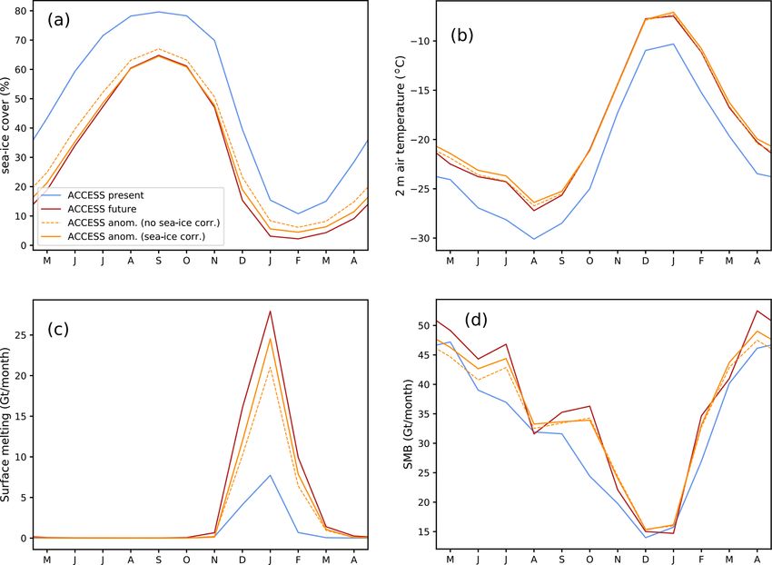
in our MAR projections. the climate-change anomaly in DJF (Fig. 10a).
These results are difficult to compare precisely to previous Over the ice sheet, the near-surface projection biases are
studies because different metrics and scenarios were used. 0.6 ◦ C in JJA and 0.2 ◦ C in DJF, which are relatively small
Based on the CMIP3 HadCM3 model under the A1B sce- compared to a warming signal of 3.5 and 3.0 ◦ C for these
nario (similar global warming as CMIP5-MMM-RCP8.5 in two seasons, respectively (Fig. 10b). Looking at the peak
2100), Kuipers Munneke et al. (2014) found that 50 % of the melt rate in January (Fig. 10c), we find that the projection
present-day firn air thickness would be depleted by ∼ 2130 bias represents 17 % of the climate-change signal vs. 34 %
for Cosgrove and ∼ 2085 for Abbot. Assuming that this cor- if no iterative method is used for sea ice. The annual SMB
responds to our 0.85 melt-to-snowfall threshold, we rather projection bias represents 16 % of the projected increase vs.
find ∼ 2055 for Cosgrove and ∼ 2100 for Abbot. Moreover, 32 % if no iterative method is used for sea ice (Fig. 10d). In
Kuipers Munneke et al. (2014) found little firn air depletion terms of spatial pattern, the climate-change signal remains
by 2200 under A1B for all the ice shelves from Thwaites significantly larger than the projection bias at most locations
to Getz, while we find that firn air could be fully depleted (Fig. 11a, b). The melt projection bias is positive at most
at Getz and Dotson before 2200. The generally later full- melting locations with a bias consistently smaller than the
depletion dates in their simulations could be related to the climate-change signal (Fig. 11c, d).
∼ −1.5 ◦ C present-day bias in the regional atmospheric sim- To summarise our assessment of our projection method,
ulations used to drive their firn model. To estimate the like- it has the advantage to start from a present-day state that
lihood of ice-shelf collapse in future scenarios, Trusel et al. is not affected by present-day biases in CMIP5 models and
(2015) used melt-rate thresholds (based on pre-collapse ob- to be applicable to a multi-model-mean projection which is
servations at Larsen B). They found that only Abbot could expected to remove a part of the CMIP5 model biases. The
reach this threshold by 2100 and only under the RCP85 sce- counterpart of these advantages are biases in the projection it-
nario, but given the large snowfall spatial variability around self. These biases are estimated to remain below 20 % based
Antarctica and across the Amundsen region, we believe that on our perfect-model approach. A part of these biases may
the melt-to-snowfall ratio would be a better indicator of po- be related to the imperfect method used to apply the sea-
tential ice-shelf collapse than a uniform melt-rate threshold ice anomaly. Using iterative absolute anomalies typically re-
as used in Nowicki et al. (2020) and Seroussi et al. (2020). moves half of the projection biases compared to a simple
absolute anomaly, but the bias is not completely removed
4.2 Modelling and methodological limitations in summer, and more iterations or a refined method may be
needed in our approach. Alternative approaches to build fu-
We now assess the ability of our projection method to cap- ture sea-ice concentrations were proposed by Beaumet et al.
ture the future climatology in a similar way to Yoshikane (2019b), and some of them may be more effective at remov-
et al. (2012), i.e. running a perfect-model test (i.e. assum- ing projection biases, although their approaches produced bi-
ing that the future is perfectly known by considering that ases of similar magnitude as our iterative absolute anomaly
a given projection is true). To do so, we now consider a method (their Fig. 5). Another possible cause for our pro-
The Cryosphere, 15, 571–593, 2021 https://doi.org/10.5194/tc-15-571-2021M. Donat-Magnin et al.: Amundsen projections 583 Figure 9. Extrapolated melt-to-snowfall ratio as a function of warming with respect to the present day (solid lines correspond to Eq. 2 and dashed lines to Eq. 3). The values obtained through our simulations correspond to the intersections with the vertical solid grey line. The vertical dashed grey lines represent warming at other dates (the dates indicated above the lines are the central years of 20-year averages) and under alternative scenarios (RCP2.6 and RCP4.5). This warming is derived from Collins et al. (2013) (their Table 12.2) assuming that the regional warming remains equal to global warming (supported by our results, as well as Collins et al., 2013). The corresponding warming for the CMIP6 multi-model mean (see list in Appendix A) under scenarios SSP126, SSP245, and SSP585 are indicated as vertical thin dashed rosy-brown lines. The horizontal black lines indicate three indicative thresholds for a net production of surface liquid water: the future 0.60 ratio simulated at Abbot in 2080–2100 (which is the minimum ratio for which we detect a significant production of surface liquid water), the 0.70 ratio estimated by Pfeffer et al. (1991), and the 0.85 ratio for which more than 50 % of the grid points experience a net production of surface liquid water (Fig. 7). The warming range for which the extrapolations cross the 0.60 and 0.85 thresholds are indicated by the horizontal colour bars at the bottom. jection biases is the fact that we assume unchanged inter- the projection bias is not expected to change the list of ice annual variability with respect to the mean in the projected shelves experiencing a future production of surface liquid future, while the true future experiences a different variabil- water. Moreover, the melt rates and snowfall produced by ity. Changes in inter-annual variability or extreme events may MAR in this configuration were shown to be biased by typi- indeed affect non-linear processes (e.g. melt rates vary ex- cally −20 % and +20 %, respectively (Donat-Magnin et al., ponentially with temperatures) even if the mean is the same 2020b), although observational melt-rate products are also in the true future and the projected future. Notwithstand- highly uncertain (Datta et al., 2019). Increasing melt rates ing these limitations, we consider that our methodology has in Table 2 by 20 % and reducing snowfall by 20 % changes some advantages and should be used for projections, together the melt-to-snowfall ratios, bringing Abbot’s to 0.92, i.e. well with other existing methods. above the critical threshold. This again shows the high sen- We now discuss the consequences of the aforementioned sitivity of projected surface liquid water production at the model and methodological biases for future surface liquid surface of Abbot. Nonetheless, Thwaites (ratio changed to water production and potential hydrofracturing. Our pro- 0.37), Crosson (0.20), Dotson (0.53), and Getz (0.51) main- jection method produces an underestimation of both snow- tain a low probability to experience a net production of sur- fall and melt rates in the future by 16 % to 17 %. Adding face liquid water even accounting for possible model biases. these errors to both snowfall and melting values in Table 2 These estimates suggest that the absence of liquid water at would keep the melt-to-snowfall ratio unchanged. As such, https://doi.org/10.5194/tc-15-571-2021 The Cryosphere, 15, 571–593, 2021
584                                                                                M. Donat-Magnin et al.: Amundsen projections

Figure 10. Mean 21-year seasonal cycle of (a) domain-averaged sea-ice concentration, (b) 2 m air temperature, (c) surface melt, and (d) SMB,
with (b–d) integrated over the seven glacial drainage basins from Getz to Abbot (including both ice shelf and grounded ice). The blue and
dark-red lines correspond to the present and true future based on ACCESS-1.3, respectively. The orange lines represent the results of the
projected future, applied with (solid) and without (dashed) sea-ice iterative correction (see Sect. 2).

the surface of Thwaites, Crosson, Dotson, and Getz in 2100              production associated with a melt-to-snowfall ratio close to
under CMIP5-MMM-RCP8.5 conditions is a robust feature.                  the critical threshold, which probably means that the firn is
   We now discuss another critical aspect of firn modelling,            still slowly filling up after 12 years. Expanding the spin-up
which is the spin-up duration. Our approach has consisted               duration much further under constant 2080–2100 conditions
of running a present and a future 30-year snapshot, which               would not make a lot of sense as earlier conditions were less
means that the future firn has not experienced transient                affected by climate warming. We suggest that simulating the
changes throughout the 21st century. Instead, we have run a             transient 21st century may be needed to set up the future firn
12-year spin-up under future conditions for every simulated             properties of Abbot, and our results concerning this ice shelf
year of the future experiment (the years are run in parallel).          therefore have to be considered carefully.
We now consider surface liquid water produced in DJF 1998
with climate anomalies on top, which is the summer with
the highest melt rates in our projection and is preceded by             5   Conclusion
a decade of relatively high melt rates (Donat-Magnin et al.,
2020b). We consider that the spin-up duration is sufficiently           In this study, we have presented future projections of SMB
long if the net production of surface liquid water in DJF               and surface melt at the end of the 21st century under the
1998 reaches a steady state for spin-up durations shorter than          RCP8.5 scenario based on the MAR regional atmospheric
12 years. Whatever the spin-up duration, there is no signifi-           model at 10 km resolution. The climate-change anomaly is
cant net production at the surface of Getz, Dotson, Crosson,            calculated from the seasonal climatology of a CMIP5 multi-
or Thwaites (Fig. 12), which is expected due to the low melt-           model mean, and added to the ERA-Interim reanalysis which
to-snowfall ratio (see previous section). For Pine Island and           is used for present-day boundary conditions. The use of an
Cosgrove, an approximate steady state seems to be reached               anomaly has the advantage to start from a present state with
after 6–7 years, although the net production at Cosgrove still          small biases compared to observations and is expected to re-
experiences fluctuations of ±10 %. In contrast, the net pro-            duce future biases as most CMIP5 biases were shown to be
duction over Abbot is still drifting after 12 years of spin-up.         stationary. Moreover, the use of a multi-model mean is ex-
This is likely related to the relatively weak but non-zero net          pected to cancel the biases that are not common to a majority
                                                                        of models. An important caveat of this method is that we as-

The Cryosphere, 15, 571–593, 2021                                                              https://doi.org/10.5194/tc-15-571-2021
M. Donat-Magnin et al.: Amundsen projections 585
Figure 11. (a) SMB anomaly (2080–2100 minus 1989–2009) in ACCESS-1.3 directly downscaled by MAR (i.e. true changes). (b) Difference
between the true future, from the direct downscaling of ACCESS-1.3, and the projected future, from the anomaly method. (c, d) Same as (a, b)
but for melt rates instead of SMB. The dark red contours in panel (a) indicate individual glacial drainage basins: Getz (GET), Dotson (DOT),
Crosson (CRO), Thwaites (THW), Pine Island Glacier (PIG), Cosgrove (COS), and Abbot (ABB). Red hatching in (c) indicates ice shelves.
The ice-sheet topography is shown in grey (contours every 400 m).
sume unchanged inter-annual variability with respect to the
mean. A perfect-model test indicates that our approach cap-
tures future changes in most variables despite an underesti-
mation of SMB and melt-rate changes by 17 % on average.
Considering the drainage basins of the seven major ice
shelves from Getz to Abbot, and only for the grounded parts
of the ice sheet, we find that SMB increases from 336 to
455 Gt yr−1 throughout the 21st century, which would reduce
the global sea level changing rate by 0.33 mm yr−1 . Even
in the future climate, SMB over the grounded ice sheet re-
mains nearly equivalent to snowfall in this region. Snowfall
increases by 7.4 to 8.9 % ◦ C−1 of near-surface air warming,
which is similar to global warming in this region. This sensi-
tivity is slightly larger than previous estimates for the whole
ice sheet (Palerme et al., 2017; Lenaerts et al., 2016; Ligten-
berg et al., 2013, and references therein) and larger than pre-
dicted by Clausius–Clapeyron (increase in saturation vapour
Figure 12. Net production of surface liquid water over individual
pressure by 7 to 7.5 % ◦ C−1 ). This may be explained by a de-
ice shelves in DJF 1998 for various spin-up durations for Getz, Dot-
son, Crosson, Thwaites, Pine Island Glacier (PIG), Cosgrove, and
creased sea-ice cover along the ice-sheet margin which helps
Abbot. near-surface air masses to reach their water vapour satura-
tion. Changes in local circulation in autumn and the associ-
https://doi.org/10.5194/tc-15-571-2021 The Cryosphere, 15, 571–593, 2021You can also read