Ice and mixed-phase cloud statistics on the Antarctic Plateau
←
→
Page content transcription
If your browser does not render page correctly, please read the page content below
Atmos. Chem. Phys., 21, 13811–13833, 2021
https://doi.org/10.5194/acp-21-13811-2021
© Author(s) 2021. This work is distributed under
the Creative Commons Attribution 4.0 License.

Ice and mixed-phase cloud statistics on the Antarctic Plateau
William Cossich1, , Tiziano Maestri1, , Davide Magurno1, , Michele Martinazzo1 , Gianluca Di Natale2 ,
Luca Palchetti2 , Giovanni Bianchini2 , and Massimo Del Guasta2
1 Physicsand Astronomy Department, Alma Mater Studiorum – University of Bologna, Italy
2 Istituto
        Nazionale di Ottica, Consiglio Nazionale delle Ricerche, Italy
 These authors contributed equally to this work.

Correspondence: Tiziano Maestri (tiziano.maestri@unibo.it)

Received: 1 February 2021 – Discussion started: 23 March 2021
Revised: 24 August 2021 – Accepted: 26 August 2021 – Published: 17 September 2021

Abstract. Statistics on the occurrence of clear skies, ice        warming. Monthly mean results are compared to cloud oc-
clouds, and mixed-phase clouds over Concordia Station, in         currence and fraction derived from gridded (Level 3) satellite
the Antarctic Plateau, are provided for multiple timescales       products from both passive and active sensors. The differ-
and analyzed in relation to simultaneous meteorological pa-       ences observed among the considered products and the CIC
rameters measured at the surface. Results are obtained by         results are analyzed in terms of footprint sizes and sensors’
applying a machine learning cloud identification and clas-        sensitivities to cloud optical and geometrical features. The
sification (CIC) code to 4 years of measurements between          comparison highlights the ability of the CIC–REFIR-PAD
2012–2015 of downwelling high-spectral-resolution radi-           synergy to identify multiple cloud conditions and study their
ances, measured by the Radiation Explorer in the Far Infrared     variability at different timescales.
– Prototype for Applications and Development (REFIR-
PAD) spectroradiometer. The CIC algorithm is optimized
for Antarctic sky conditions and results in a total hit rate
                                                                  1   Introduction
of almost 0.98, where 1.0 is a perfect score, for the identi-
fication of the clear-sky, ice cloud, and mixed-phase cloud       The polar regions present several challenges for meteorology
classes. Scene truth is provided by lidar measurements that       and climatology studies (Walsh et al., 2018). These regions
are concurrent with REFIR-PAD. The CIC approach demon-            are crucial components of the Earth’s radiation budget (ERB)
strates the key role of far-infrared spectral measurements for    (Liou, 2002; Kiehl and Trenberth, 1997) since they gener-
clear–cloud discrimination and for cloud phase classification.    ally emit more energy to space in the form of infrared radi-
Mean annual occurrences are 72.3 %, 24.9 %, and 2.7 % for         ation than what is absorbed from sunlight, thereby behaving
clear sky, ice clouds, and mixed-phase clouds, respectively,      as heat sinks. Modeling studies have shown that changes in
with an inter-annual variability of a few percent. The sea-       cloud properties (e.g., cloud amount, cloud thermodynamic
sonal occurrence of clear sky shows a minimum in winter           phase, cloud height, cloud optical thickness) over Antarctica
(66.8 %) and maxima (75 %–76 %) during intermediate sea-          may impact different regions in the globe, highlighting the
sons. In winter the mean surface temperature is about 9 ◦ C       importance of Antarctic clouds for the global climate sys-
colder in clear conditions than when ice clouds are present.      tem (Lubin et al., 1998). However, obtaining measurements
Mixed-phase clouds are observed only in the warm season; in       of cloud properties in the Antarctic continent is still a chal-
summer they amount to more than one-third of total observed       lenge (Silber et al., 2018; Lubin et al., 2020), especially in its
clouds. Their occurrence is correlated with warmer surface        interior (Town et al., 2005; Lachlan-Cope, 2010; Bromwich
temperatures. In the austral summer, the mean surface air         et al., 2012). Observations from synoptic weather stations re-
temperature is about 5 ◦ C warmer when clouds are present         quire an experienced observing staff and sometimes become
than in clear-sky conditions. This difference is larger during    unavailable during “white-out” conditions caused by blowing
the night than in daylight hours, likely due to increased solar   snow. Analysis of satellite measurements from both active

Published by Copernicus Publications on behalf of the European Geosciences Union.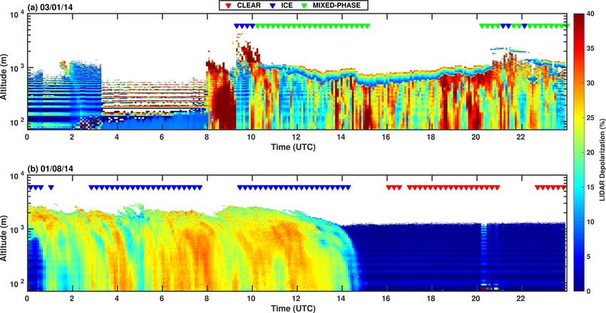
13812                                                                W. Cossich et al.: Cloud occurrence on the Antarctic Plateau

and passive sensors must account for a number of problems               ering the 100–700 cm−1 band. Many studies have shown
in inferring the cloud properties. One issue is that the cloud          that the FIR can be used to complement standard remote
radiative properties tend to be very similar to those of the            sensing measurements performed in the mid-infrared (MIR)
background (the snow or ice surface). Optically thin cirrus             and improve cloud detection, classification, and inference of
clouds are often present in the Antarctic Plateau (King and             cloud properties (Rathke et al., 2002; Palchetti et al., 2016;
Turner, 1997) but are difficult to identify and analyze due             Di Natale et al., 2017; Maestri et al., 2019a). Moreover,
to their small cloud signals (the difference between cloudy             ground-based remote sensing spectral upwards-looking mea-
and clear-sky radiances). Measurements become problematic               surements are very useful to determine the cloud properties
during the long polar night (King and Turner, 1997), and                relevant to the energy budget (Mahesh et al., 2001; Cox et al.,
some stations reduce the observing frequency in the winter              2014; Di Natale et al., 2020).
time (Bromwich et al., 2012). Observations at solar wave-                  This study is performed in this context and exploits a
lengths are not available for about half of the year, thus re-          unique dataset derived from FIR and MIR downwelling
ducing the overall ability to recognize the presence of cloud           spectral radiances measured at Concordia Station, Dome
layers and to derive their physical and optical features. Mea-          C, in the middle of the Antarctic Plateau. The measure-
surements at longer wavelengths (i.e., in the infrared, IR) are         ments are performed by means of the Radiation Explorer
available regardless of solar illumination, but, frequently, the        in the Far Infrared – Prototype for Applications and De-
cloud top temperature is similar to the ice surface temper-             velopment (REFIR-PAD) Fourier transform spectroradiome-
ature (King et al., 1992; King and Turner, 1997; Bromwich               ter (Bianchini et al., 2019) in the scope of the projects Ra-
et al., 2012), and the cloud identification is thus difficult from      diative Properties of Water Vapor and Clouds in Antarctica
passive satellite observations.                                         (PRANA) and Concordia Multi-Process Atmospheric Stud-
   Active remote sensing techniques have been very helpful              ies (CoMPASs), within the Italian National Program for Re-
in overcoming the limitations of the passive instruments in             search in Antarctica (PNRA; Palchetti et al., 2015). These
polar regions. Adhikari et al. (2012) investigated the sea-             projects represent the first long-term field campaigns to col-
sonal and inter-annual variabilities in the vertical and hor-           lect high-spectral-resolution radiances in the FIR, with conti-
izontal cloud distributions over the southern high latitudes            nuity for an extended period (measurements started in 2012).
poleward of 60◦ S, using observations from CloudSat and                 REFIR-PAD is installed inside an insulated shelter, named
Cloud–Aerosol Lidar and Infrared Pathfinder Satellite Ob-               the Physics Shelter, together with a backscattering lidar (ab-
servation (CALIPSO) satellites between June 2006 and May                breviation of light detection and ranging). The lidar de-
2010. They found that the Antarctic Plateau has the low-                tects backscattering and depolarization signals up to 7 km
est cloud occurrence of the Antarctic continent (< 30 %).               above the surface. Besides these measurements, the Antarc-
The sensors on board the aforementioned satellites have also            tic Meteo-Climatological Observatory installed at Concor-
been used to investigate macro- and microphysical Antarc-               dia (http://www.climantartide.it/, last access: 14 Septem-
tic cloud properties (Verlinden et al., 2011; Adhikari et al.,          ber 2021) provides data from an automatic weather station
2012; Listowski et al., 2019; Ricaud et al., 2020). Never-              (AWS) and from daily radiosonde launches. These measure-
theless, satellite active sensors are not lacking in problems           ments are analyzed and correlated to the meteorological con-
when used for cloud detection in polar regions. For example,            ditions observed at Concordia Station and are considered rep-
Chan and Comiso (2011, 2013) discuss the difficulties en-               resentative of a large area of East Antarctica because of the
countered by the Cloud Profiling Radar (CPR), on CloudSat,              horizontal uniformity in the Antarctic Plateau.
and the Cloud–Aerosol Lidar with Orthogonal Polarization                   Recently, Maestri et al. (2019b) presented an algorithm
(CALIOP), on CALIPSO, in detecting low-level clouds in                  to identify and classify clouds based on principal compo-
the Arctic. The difficulties arise from the CloudSat coarse             nent analysis of IR radiance spectra at high spectral reso-
vertical resolution (about 500 m) and its limited sensitivity           lution. The cloud identification and classification (CIC) is a
(low signal-to-noise ratio) near the surface and in the case of         fast machine learning algorithm able to perform a cloud de-
CALIOP are due to the geometrically thin nature of the cloud            tection and classification, exploiting spectral variations in IR
and its surface proximity. Bromwich et al. (2012) present a             radiance signals. CIC can account for spectral radiance from
review of Antarctic tropospheric clouds. They discuss the in-           the full IR spectrum including the MIR and FIR. The algo-
struments and methods to observe Antarctic clouds and the               rithm analyzes a distribution of the so-called similarity index,
current datasets available. The authors highlight that there are        which is a parameter defining the level of closeness between
relatively few measurements of clouds in the Antarctic, espe-           the analyzed spectra and the elements of specific classes that
cially in the interior. They also indicate that better and more         are defined with training sets.
frequent remote sensing and in situ observations are needed.               In this study, the CIC algorithm is applied to REFIR-
   The selection of the FORUM project (Palchetti et al.,                PAD downwelling radiances to detect and classify Antarctic
2020) in 2019 as the ninth Earth Explorer mission by the                clouds between 2012 and 2015. The main goal of this effort
European Space Agency (ESA) has revitalized studies in the              is to obtain statistics on clear-sky and cloud occurrence as
far-infrared (FIR) part of the spectrum, approximately cov-             well as the investigation of the diurnal cycle and seasonality

Atmos. Chem. Phys., 21, 13811–13833, 2021                                               https://doi.org/10.5194/acp-21-13811-2021
W. Cossich et al.: Cloud occurrence on the Antarctic Plateau                                                                13813

                                                                   station opened in 2005 as part of an international cooper-
                                                                   ation project between the Italian National Program for Re-
                                                                   search in Antarctica (PNRA) and the French Polar Institute
                                                                   Paul-Émile Victor (IPEV). A detailed description of the in-
                                                                   strumentation available in the PRANA and CoMPASs exper-
                                                                   iments at Concordia Station is given in Palchetti et al. (2015).
                                                                   A brief overview of the instruments and measurements made
                                                                   between 2012 and 2015 is provided in what follows.
                                                                      Spectral measurements of the downwelling radiance are
                                                                   performed by REFIR-PAD, which provides spectrally re-
                                                                   solved zenith-looking radiance measurements in the range
                                                                   100–1500 cm−1 , with a 0.4 cm−1 spectral resolution, thus
                                                                   covering a large part of the atmospheric longwave emission,
                                                                   including both the FIR and part of the MIR region. The in-
                                                                   strument points at the zenith through a 1.5 m chimney. The
                                                                   measurement sequence to obtain one complete spectrum is
                                                                   made of four calibration acquisitions, in which the instru-
                                                                   ment looks at the internal reference blackbody sources, and
                                                                   four sky observations. Each single acquisition takes about
                                                                   80 s. The entire sequence has a duration of about 14 min:
                                                                   5.5 min of sky observations, 5.5 min of calibrations, and
Figure 1. Antarctica elevation map, with Concordia Station indi-   delays for detector settling after scene changes (Palchetti
cated by a red star.
                                                                   et al., 2015). REFIR-PAD is a fast-scanning spectroradiome-
                                                                   ter with signals acquired in the time domain and resampled in
Table 1. Number of analyzed REFIR-PAD spectra for each year.       postprocessing at equal intervals in optical path difference. It
                                                                   has been designed to operate with uncooled detectors and op-
         Year        2012     2013      2014     2015              tics. The instrument operates full-time, with alternating cy-
         Spectra   16 177    19 298   25 089    27 396             cles of 5–6 h of measurements and 1–3 h of analysis. It is in-
                                                                   stalled in the Physics Shelter, located 500 m southward from
                                                                   the main station, in what is called the clean-air area, where
of clouds in the Antarctic Plateau. Both ice and mixed-phase       the predominant winds keep the air clean from the exhaust
clouds have been considered, the latter consisting of a su-        plume of the Concordia power generator. Between the years
percooled liquid water layer that, in general, may have ice        2012 and 2015, a total of 87 960 spectra were analyzed. The
particles present either above or below (usually precipitating     spectra annual distribution is reported in Table 1.
in this case).                                                        Since 2005, Concordia Station has provided hourly mea-
   The algorithm is first applied to a test set so that the        surements of air temperature, pressure at the surface level,
CIC performances are assessed. The excellent classification        relative humidity, wind speed, and wind direction. The snow
scores obtained in the testing phase provide a solid base for      temperature is measured at different depths from 5 cm to
the application of the CIC to the entire dataset. In this study,   10 m. These measurements began in December 2012. Ra-
an effort is made to link the meteorological state of the atmo-    diosondes (Vaisala RS92) have been routinely released ev-
sphere to the cloud occurrence.                                    ery day at 12:00 UTC since 2006. They reach an altitude of
   The paper is organized as follows. Section 2 describes the      about 18 km in wintertime and about 25 km in the summer.
instrumentation and measurements performed at Concordia            All these data are made available by the Antarctic Meteo-
Station. Section 3 introduces the CIC algorithm, its setup,        Climatological Observatory, and a subset of them is used in
and optimization to identify and classify clouds. Section 4        this study.
discusses the cloud occurrence results at different timescales.       Atmospheric backscattering and depolarization ratio
The study is summarized in Sect. 5, where conclusions are          (cross-polarized over parallel-polarized total signal) pro-
drawn.                                                             files are measured by a lidar every 5 min (Palchetti
                                                                   et al., 2015). The instrument (http://lidarmax.altervista.org/
                                                                   englidar/Antarctic%20LIDAR.php, last access: 14 Septem-
2   Instrumentation and measurements                               ber 2021) is a Hamamatsu analog photo-multiplier tube, op-
                                                                   erating a Quantel laser (Brio) at 532 nm with a biaxial con-
Concordia Station is an Antarctic research base located at         figuration (10 cm off-axis) and nominal laser aperture of
Dome C over the Antarctic Plateau (75◦ 060 S, 123◦ 230 E;          1 mrad full angle. The lidar telescope has refractive optics
3.230 m a.m.s.l.), in the East Antarctic region (Fig. 1). The      with 10 cm diameter and 30 cm focal length, with a field

https://doi.org/10.5194/acp-21-13811-2021                                        Atmos. Chem. Phys., 21, 13811–13833, 2021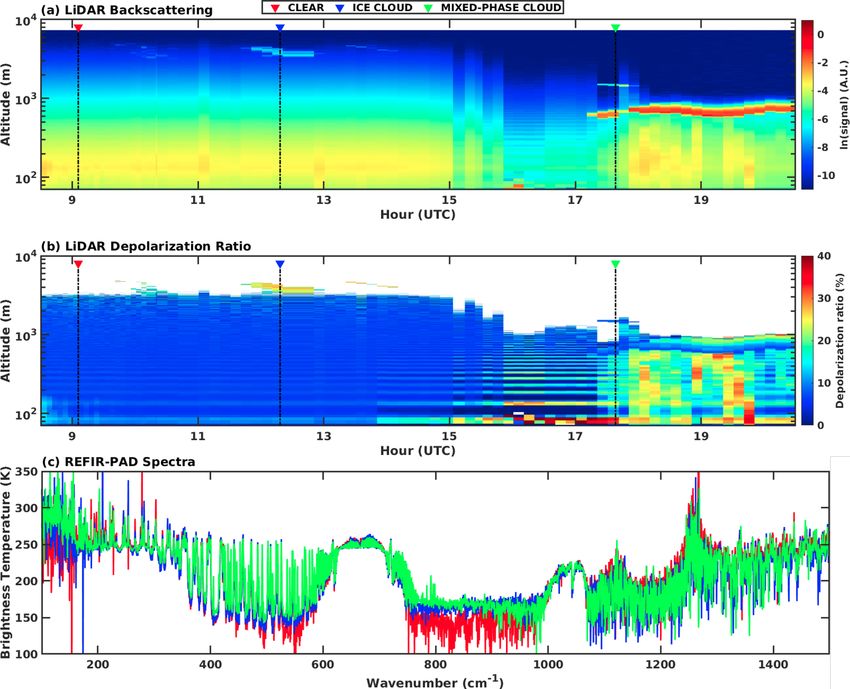
13814                                                             W. Cossich et al.: Cloud occurrence on the Antarctic Plateau

of view of approximately 2 mrad full angle. An interference          nal increases in the presence of cloud particles. As shown
bandpass filter of 0.15 nm bandwidth is applied. The signal is       in the figure, clouds can be composed of multiple layers,
averaged over 1000 laser shots. Measurements range from 30           each one with different depolarization features. When the
to 7000 m above the surface, with 7.5 m vertical resolution.         depolarization ratio is higher than 15 %, the cloud is clas-
The line of sight is 4◦ off-zenith to avoid possible ambiguity       sified as an ice cloud (blue triangle). For lower values of
between liquid-phase clouds and oriented ice plates (Ricaud          the depolarization ratio, it is assumed that the layer contains
et al., 2020). The lidar operates through a window to enable         the liquid phase, and the cloud is categorized as a mixed-
measurements in all weather conditions.                              phase cloud (green triangle). The 15 % depolarization ratio
                                                                     value is selected to account for the impact of multiple scat-
Definition of classes                                                tering within liquid clouds. It is observed that in the pres-
                                                                     ence of mixed-phase clouds the depolarization ratio shows
A subset of REFIR-PAD data, comprising 1928 spectra, is              very small values at the cloud base, characteristics of liquid
co-located with lidar measurements. The co-location crite-           spheres, and increases towards values typical of ice crystals
rion is defined by the time of measurements: each REFIR-             near the cloud top. An increase is, in part, intrinsically related
PAD spectrum is associated with the lidar data that are clos-        to liquid water layers, where multiple scattering determines
est in time. Co-located measurements are used to classify the        a depolarization that gradually increases with the depth of
REFIR-PAD spectra. For these cases, cloud layers are de-             penetration. For this reason, in some conditions, the phase
tected from the analysis of the backscatter profiles, and the        of the upper part of the cloud cannot be unambiguously de-
depolarization ratio is used to determine the thermodynamic          fined based on the analysis of the depolarization ratio profile
phase of the particles. The classified spectra are then used         only. Nevertheless, the presence of the liquid phase at the bot-
to set up training and test sets as described in more detail in      tom is unequivocally identified, and the cloud is categorized
the next section. In the Antarctic environment the determina-        as mixed-phase. The occurrence of precipitating ice crystals
tion of cloud thermodynamic phase is not trivial. According          from mixed-phase cloud layers is not infrequent, even if in
to Liou and Yang (2016), liquid water droplets retain the po-        very small quantities.
larization state of the incident energy, while the light beam
backscattered from non-spherical ice particles is partially de-
polarized as a result of internal reflections and the transfor-      3   Cloud identification and classification algorithm
mation of coordinate systems governing the electric vector.
                                                                     The Cloud Identification and Classification (CIC) is a ma-
A theoretical analysis performed by the same authors shows
                                                                     chine learning algorithm, based on the principal component
that in the presence of a liquid water cloud the depolariza-
                                                                     analysis (PCA), that is able to classify an input spectrum (L)
tion remains at about 2 %–4 %, whereas radiation backscat-
                                                                     as representative of a specific class, characterized by the ele-
tered from non-spherical ice particles is strongly depolar-
                                                                     ments contained in multiple groups of spectra used as train-
ized, varying between 30 % and 40 %. However, the thresh-
                                                                     ing sets (TSs). The algorithm is based on the analysis of the
old to determine the water physical state in real clouds can
                                                                     measured spectra only and does not require any ancillary in-
vary depending on the atmosphere and the cloud microphys-
                                                                     formation or forecast model output data for the classifica-
ical parameters. Sassen and Hsueh (1998) evaluate ground-
                                                                     tion. The classification accounts for the spectral features of
based lidar data in the presence of contrail cirri during the
                                                                     the observed brightness temperature (BT) compared to the
Subsonic Aircraft: Contrail and Cloud Effects Special Study
                                                                     characterizing spectral features of each training set. A brief
(SUCCESS) field campaign. They found depolarization ra-
                                                                     description of the algorithm is provided below; we recom-
tios in persisting contrails ranging from about 0.3 to 0.7.
                                                                     mend the reference article by Maestri et al. (2019b) for a full
Freudenthaler et al. (1996) observed depolarization ratios of
                                                                     description of the CIC.
0.1 to 0.5 for contrails with temperatures ranging from −60
                                                                        For each class X (i.e., clear-sky, ice cloud, and mixed-
to −50 ◦ C, depending on the stage of their growth. In this
                                                                     phase) a set of spectra is used to set up a training set defining
study, a depolarization ratio of 0.15 is used as a threshold
                                                                     the variability within the class:
(as indicated by Sassen, 1991) for the discrimination of the
liquid water clouds and ice clouds over Concordia Station.           TSX = TSX (ν̃, j ),                                           (1)
The value accounts for possible increases due to multiple-
scattering effects as discussed below.                               where ν̃ is the wavenumber, and j = 1, . . ., J refers to the
   An example of lidar observations for clear sky (red tri-          j th element (spectrum) of the TS. The information content
angle), ice clouds (blue triangle), and mixed-phase clouds           of the TSs is evaluated by computing the eigenvalues (λ) and
(green triangle) is provided in the upper (backscattered sig-        the eigenvectors (TS) of the TS covariance matrices:
nal) and middle (depolarization ratio) panel of Fig. 2. The          [λX , TSX ] = eig(cov(TSX )).                                (2)
lower panel of the same figure provides the correspond-
ing REFIR-PAD spectra. In clear-sky conditions, the lidar              The procedure also accounts for a spectral noise removal
backscattering signal decreases with altitude, while the sig-        operation. This is performed by accounting only for a lim-

Atmos. Chem. Phys., 21, 13811–13833, 2021                                             https://doi.org/10.5194/acp-21-13811-2021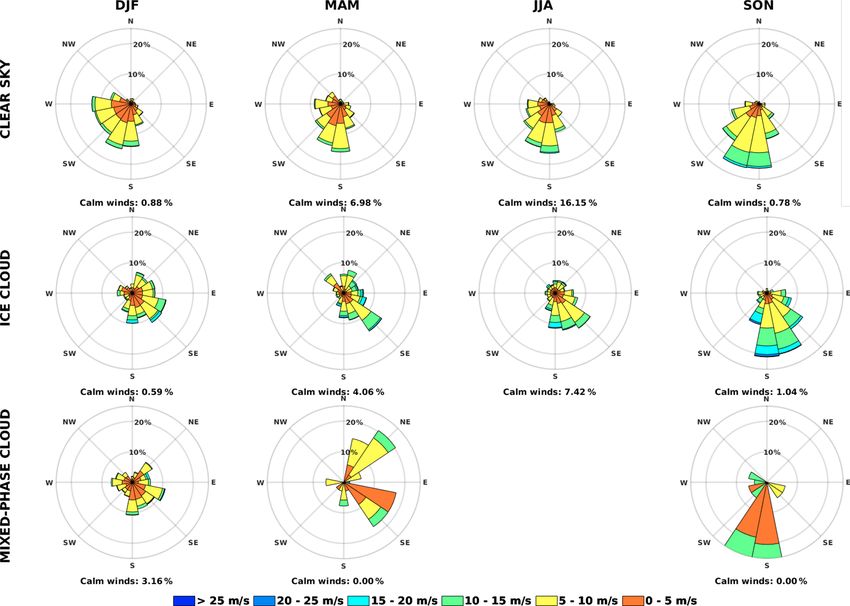
W. Cossich et al.: Cloud occurrence on the Antarctic Plateau                                                                             13815

Figure 2. (a) Lidar backscattering and (b) depolarization ratio for 2 January 2013. (a, b) Different sky conditions are highlighted by a vertical
dashed line. A red triangle indicates clear sky, a blue triangle is used for ice clouds, and a green triangle is used for mixed-phase clouds. (c)
REFIR-PAD spectra corresponding to the three sky conditions highlighted in the upper and middle panels. The same color code is used.

ited number of principal components, defined by Turner et al.              and by computing the eigenvectors (ETS) of each ETS co-
(2006) as the first P0 eigenvalues, out of P total components              variance matrix.
that minimize the indicator function:                                        The classification is performed through a parameter called
                                                                           similarity index (SI) that evaluates the variation in the infor-
             RE(p)
IND(p) =             ,                                            (3)      mation content in the ETS with respect to the original TS (for
            (P − p)2                                                       each class):
where p = 1, . . ., P −1 refers to the pth principal component,                              P0 X
                                                                                         1 X
and the real error RE is defined as                                        SIX = 1 −               |ETSX (ν̃, p)2 − TSX (ν̃, p)2 |.        (6)
          sP                                                                            2P0 p=1 ν̃
               P
               i=p+1 λX,i
RE(p) =                    .                                (4)               The SI is a normalized index, where a value close to 1
              J (P − p)                                                    means high similarity, and a value close to 0 means low
   Each input spectrum L is then analyzed by defining the                  similarity. As an example, if the input spectrum is mea-
extended training sets (ETSs) that are the original TSs plus               sured in clear-sky conditions, the information content of the
the input spectrum itself,                                                 ETSCLEAR would be similar to the original TSCLEAR , and
                                                                           their eigenvectors will also be very similar due to the low
ETSX = [TSX (ν̃, j ), L(ν̃)],                                     (5)      additional information content from the input spectrum.

https://doi.org/10.5194/acp-21-13811-2021                                                  Atmos. Chem. Phys., 21, 13811–13833, 2021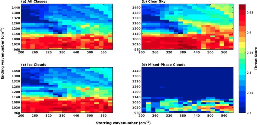
13816                                                                W. Cossich et al.: Cloud occurrence on the Antarctic Plateau

Figure 3. Logical diagram of the classification process performed by the CIC algorithm for the definition of the clear-sky, ice cloud, and
mixed-phase cloud classes.

Figure 4. Example of (a) the CIC elementary approach and (b) the distributional approach applied to the training set elements of clear sky (49
spectra) and mixed-phase clouds (22 spectra) in the warm season (November–March). The clear-sky (blue histogram) and the mixed-phase
cloud (red histogram) training set elements are classified according to the SID as clear-sky (shaded blue area) or mixed-phase cloud (shaded
red area) scenes. Only 76 % of the spectra are correctly classified using the elementary approach, while 99 % of the spectra are correctly
classified using the distributional method.

Atmos. Chem. Phys., 21, 13811–13833, 2021                                                  https://doi.org/10.5194/acp-21-13811-2021
W. Cossich et al.: Cloud occurrence on the Antarctic Plateau                                                                       13817

   For this study, as previously indicated, three classes are de-     Table 2. Number of spectra used in each TS according to the macro-
fined: clear sky, ice clouds, and mixed-phase clouds. Conse-          season. The total number of spectra used in the TS is 202.
quently, three training sets are prepared, each one containing
spectra representative of that particular class. For each obser-             Season               Clear       Ice   Mixed-phase
vation the operation described in Eq. (6) is performed for 2                                       sky     cloud          cloud
classes at a time. In our case, three SIs are obtained, derived              November–March          49       30              22
from the mutual comparison of the three classes. From these,                 April–October           64       37               –
a vector of similarity index differences (SIDs) is defined:

SID(1) = SICLEAR − SIICE CLOUD
                                                                      elementary and the distributional approaches is provided in
SID(2) = SICLEAR − SIMIXED-PHASE CLOUD                                Fig. 4. The CIC is applied to the training set spectra of clear
SID(3) = SIICE CLOUD − SIMIXED-PHASE CLOUD .                   (7)    sky and mixed-phase clouds. The elementary method (left
                                                                      panel) classifies as clear sky (shaded blue area) all the spec-
   The classification of the input spectrum is performed in           tra with SID ≤ 0 and as mixed-phase cloud (shaded red area)
accordance with the logical diagram of Fig. 3. The diagram            all the spectra with SID > 0. This methodology misclassifies
shows the comparison between specific couples of SI (yel-             some of the mixed-phase cloud training set spectra (red his-
low boxes). The partial results of each comparison are rep-           togram). The distributional method (right panel) maximizes
resented by white boxes. If one class prevails over the other         the classification performance by defining a new delimiter
two, a classification is reached, and the final output is pro-        between clear-sky and mixed-phase cloud scenes. In this ex-
vided (green boxes in the figure).                                    ample, the new delimiter is set at SID = −0.15 so that most
   The comparison between the SI of the classes is called the         of the TS spectra are correctly classified. See Maestri et al.
elementary approach. This methodology is based on a very              (2019b) for a description of the computation of the delim-
simple classificator, the SID, which works properly when              iter. Once the delimiters (DELs) are defined for each class
each class is characterized by specific spectral features that        couplet, the classification is performed by using a corrected
make the elements of the class easily distinguishable from            similarity index difference (CSID):
those pertaining to other classes. This is clearly very difficult
to attain for some classes such as, for example, the clear-           CSID(1) = SICLEAR − SIICE CLOUD
sky class and the cirrus cloud class. The classification of
                                                                                  + DEL(clear−ice cloud)
clouds over the Antarctic Plateau is particularly challenging,
primarily because of the generally low cloud optical depths           CSID(2) = SICLEAR − SIMIXED-PHASE CLOUD
whose IR spectral characteristics are very similar to those of                  + DEL(clear−mixed-phase cloud)
the clear sky. The selection of the spectra contained in each         CSID(3) = SIICE CLOUD − SIMIXED-PHASE CLOUD
training set is crucial as it is in every classification algorithm.
                                                                                  + DEL(ice cloud−mixed-phase cloud) .               (8)
In fact, the selected elements must represent the entire class
characteristics and variability to perform a correct classifica-         The entire classification procedure, schematically de-
tion.                                                                 scribed in Fig. 3, is then performed by the new classifier
   Maestri et al. (2019b) suggested that better results can           CSID in place of the SID. Due to the better performance, the
be obtained when a classificator optimization is performed            distributional method is preferred and applied in this study.
a priori by using a methodology called distributional ap-
proach. When applied to a set of observations, a perfect clas-        3.1   Training and test sets
sifier would ideally generate a bimodal SID distribution for
each comparison between two classes, splitting the elements           Spectra used to populate the training sets are chosen from
in two separate groups. This class separation is difficult to         a set of pre-classified observations. The identification is per-
achieve in reality, and the amount that elements overlap de-          formed by the co-located lidar backscatter and depolarization
pends on many factors, including the spectra used to define           profiles in accordance with the criteria described in Sect. 2.
the training sets. To mitigate the issue, the CIC is applied sep-     Each training set contains a limited number of spectra from
arately to each training set element. Based on the result for         the REFIR-PAD database, aiming at describing the variabil-
each spectrum of known class, an evaluation can be made for           ity in atmospheric conditions over Concordia Station. Due
the SID distribution for the entire set of each class. Through        to the intense variations in the environmental conditions, the
this analysis of the SID distributions, an optimal SID delim-         training sets are defined for two macro-seasons: a warm sea-
iter can be defined to maximize the correct classification of         son (November–March) and a cold season (April–October).
the training set elements. The delimiters, which can be differ-       The choice is also supported by the fact that mixed-phase
ent from zero, are set according to the classification results        clouds are extremely rare in the cold macro-season. Ricaud
to optimize the algorithm performance. An example of the              et al. (2020) observed the occurrence of supercooled liq-
SID distribution based on the training set spectra and of the         uid water clouds during the warm macro-season only, with

https://doi.org/10.5194/acp-21-13811-2021                                             Atmos. Chem. Phys., 21, 13811–13833, 2021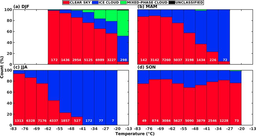
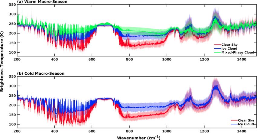
13818                                                                  W. Cossich et al.: Cloud occurrence on the Antarctic Plateau

Figure 5. Average BT (solid line) ±1 standard deviation (shaded area) for TS elements of the (a) warm and (b) cold macro-seasons.

Figure 6. Threat scores for the test set as a function of different spectral intervals ingested by the CIC algorithm. The (a) “all classes” threat
score is a weighted mean of the threat scores computed for each class: (b) clear sky, (c) ice cloud, and (d) mixed-phase cloud.

the largest frequency occurring in December and January.                   cloud training sets are used. Table 2 summarizes the number
Listowski et al. (2019) also observed that the fraction of                 of spectra for each TS and macro-season. The same spectra
supercooled liquid-water-containing clouds in the Antarctic                are used later (Sect. 4) to perform the classification of the full
Plateau varies between 10 %, in the summertime, and 0 %,                   dataset.
in winter. Therefore, three training sets for the warm macro-                 Mean spectra in terms of BT (solid lines) and their stan-
season are defined: clear sky, ice clouds, and mixed-phase                 dard deviations (shaded area) are presented in Fig. 5 for the
clouds. For the cold macro-season, only the clear-sky and ice              training sets used for both macro-seasons. Differences be-

Atmos. Chem. Phys., 21, 13811–13833, 2021                                                     https://doi.org/10.5194/acp-21-13811-2021
W. Cossich et al.: Cloud occurrence on the Antarctic Plateau                                                                   13819

tween the mean spectra of the different classes are observed          – False negative (FN): the spectrum belongs to class A,
in the window channels located between 400 and 600 cm−1                 but it is misclassified in class B or C.
as well as between 800 and 1000 cm−1 . Note that in IR win-
dow regions (transparent channels) the standard deviation of          Given the above possibilities, for each class the threat
the clear-sky spectra is usually lower than that of the cloudy      score is defined as
spectra, which account for a wider signal variability in these                   TP
bands. Furthermore, the clear-sky signal is very low at win-        ThS =                ,                                        (9)
                                                                            TP + FN + FP
dow wavenumbers, and the measurements can have a very
low signal-to-noise ratio.                                          which accounts for the correctly classified spectra (TP) in the
   Once the TSs are defined, the DELs are computed (as de-          class and penalizes all the misclassified occurrences (FN and
scribed in Sect. 3), and the CIC is ready to ingest the REFIR-      FP). A ThS value of 1 means that there are no misclassified
PAD spectra and provide their classification. To evaluate the       spectra.
CIC performance and optimize its setup, a test set of 1726             Based on the results obtained for each of the combinations
pre-classified spectra collected in 2013 is analyzed. The test      of starting and ending wavenumbers, the ThS is calculated
set is composed of 559 clear-sky, 1022 ice cloud, and 145           for each class (clear sky, ice cloud, mixed-phase cloud). The
mixed-phase cloud spectra. These spectra were previously            weighted mean ThS values, which account for the total num-
classified by using the co-located lidar backscatter and de-        ber of cases in each class, are also calculated. In the upper left
polarization profiles. An example is provided in Fig. 2. We         panel (a) of Fig. 6 the mean ThSs are plotted as a function of
define the sky condition as that observed when the REFIR-           the starting and ending wavenumbers. The other panels in
PAD starts its measurement. Then, the spectra are associated        this figure (b, c, d) show results for the three specific classes.
with the sky conditions encountered at the beginning of each        The ThS values span from 0.487 to 0.966 in accordance with
measurement.                                                        the selected interval and the given class. For intervals ending
                                                                    with wavenumbers larger than 1140 cm−1 , the ThS decreases
3.2   CIC performance and optimization                              considerably for all the classes. This is likely associated with
                                                                    the noise of the REFIR-PAD sensor, which increases consid-
The CIC algorithm is applied to the test set spectra by ac-         erably above 1200 cm−1 and degrades the classification re-
counting for their BT in different spectral intervals. This         sults. When the ending wavenumber is set to values between
operation is performed to find the optimal spectral inter-          980 and 1080 cm−1 , the ThS is very high (larger than 0.9) for
val that maximizes the classification results for each class        all the starting wavenumbers below 400 cm−1 , both for clear
(clear sky, ice cloud, mixed-phase cloud). Multiple runs of         sky and ice clouds. The spectral interval 380–1000 cm−1 per-
the CIC algorithm are performed on the same test set by ap-         forms the best for classification of both clear sky and ice
plying it to different spectral ranges. Specifically, the start-    clouds, where the ThS values are 0.963 and 0.966, respec-
ing wavenumber is moved in steps of 20 cm−1 in the 200–             tively. The classification of mixed-phase clouds is slightly
600 cm−1 band, and the ending wavenumber is moved be-               less robust compared to the other two classes, and the best
tween 960 and 1480 cm−1 . Note that, as discussed in Maestri        spectral interval is 540–1020 cm−1 with a ThS of 0.927. Typ-
et al. (2019b) and Magurno et al. (2020), the spectral interval     ically, mixed-phase clouds are associated with more humid
620–670 cm−1 is excluded from the analysis.                         conditions than ice clouds and, frequently, with precipita-
   The algorithm performance during this process is assessed        tion of thin ice crystals. For these reasons, the inclusion of
by evaluating the threat score (ThS). A confusion matrix is         the smallest wavenumbers (associated with the less transpar-
used to compute the ThS of each class and for each consid-          ent part of the FIR) does not maximize the classification of
ered spectral interval. Each individual spectrum can be clas-       mixed-phase clouds.
sified correctly as a member of its class (i.e., class A) or in-       When accounting for all the classes, the best performing
correctly as a member of a different class (i.e., class B or        spectral range for clear and cloud identification and classi-
C). With this symbolism, the spectrum classification is inter-      fication is the 380–1000 cm−1 interval. The result is depen-
preted in terms of the following.                                   dent on sensor characteristics, and for this study it is specifi-
                                                                    cally driven by the REFIR-PAD spectral resolution and noise
  – True positive (TP): the spectrum belongs to class A, and        features. The optimal interval for the classification is also de-
    it is properly classified in class A.                           pendent on many other parameters, among which are the type
                                                                    and number of classes considered, the observation geometry
  – True negative (TN): the spectrum does not belong to             (e.g., satellite- or ground-based), the observing location, and
    class A, and it is properly classified in its class of perti-   the mean atmospheric conditions. Because the water vapor
    nence (B or C).                                                 content is extremely low, the ground-based measurements on
                                                                    the Antarctic Plateau allow the full exploitation of the FIR
  – False positive (FP): the spectrum belongs to class B or         spectral range. These channels would be totally opaque for
    C, but it is misclassified in class A.                          upward observations in regions of increased water vapor con-

https://doi.org/10.5194/acp-21-13811-2021                                          Atmos. Chem. Phys., 21, 13811–13833, 2021
13820                                                                W. Cossich et al.: Cloud occurrence on the Antarctic Plateau

Figure 7. Lidar depolarization ratio on (a) 3 January 2014 and (b) 1 August 2014. The triangles mark the REFIR-PAD observations. The
color code indicates the CIC classification: red for clear sky, blue for ice clouds, and green for mixed-phase clouds.

tent such as the tropics. The selected spectral range (380–             top as suggested by the large values of the depolarization ra-
1000 cm−1 ) highlights the fundamental role of the FIR part             tio.
of the spectrum in the cloud identification and classification.            Sensitivity studies on the identification of mixed-phase
   The results of the CIC classification applied to the test set        clouds are performed assuming a cloud layer of constant to-
using the 380–1000 cm−1 are summarized in Table 3. The                  tal optical depth of 2 at 900 cm−1 , in which the base layer
table reports the number of spectra per class in the test set, the      is composed of liquid water, and the upper layer is occu-
CIC hit rates (HRs) and misclassified spectra in percentage,            pied by ice particles. The relative weight of the two layers
and the threat scores. The HR for a class (i.e., A) is defined          to the total optical depth (OD) varies from a completely ice
as                                                                      cloud to a completely liquid water cloud. Results (not shown
                                                                        here) demonstrate that for the bottom layer of liquid phase
         NACIC      TP
HRA =           =         ,                                  (10)       with OD larger than 0.1–0.3 the cloud is identified as mixed-
         NAtrue   TP + FN                                               phase; otherwise, it is classified as an ice cloud. This demon-
                                                                        strates that the algorithm is very sensitive to the presence of
where NACIC is the number of occurrences of the class A that
                                                                        thin liquid water layers at the cloud base. Nevertheless, it is
are correctly identified by the CIC (corresponding to the TP
                                                                        also possible to incur in situations in which a very thin layer
in the confusion matrix). NAtrue is the total number of ele-
                                                                        of liquid water is close to a thicker ice layer, and the spectral
ments in class A of the dataset and corresponds to TP+FN of
                                                                        signal measured at the ground is interpreted by the CIC al-
the class A.
                                                                        gorithm as exiting from an ice cloud. Another common situ-
   The overall performance is that almost 98 % of spectra
                                                                        ation is the presence of falling ice from mixed-phased cloud
are correctly classified. Only a small percentage (less than
                                                                        layers, as shown in the mid panel of Fig. 2 between 18:00
1 %) of cloudy spectra (ice clouds plus mixed-phase clouds)
                                                                        and 20:00 UTC. Typically, the quantity of the precipitating
are misclassified as clear sky, and about 2 % of the clear-sky
                                                                        ice crystals is very small, and the CIC algorithm is able to
spectra are erroneously identified as ice clouds. Note that in
                                                                        capture the radiometric signal from the upper liquid water
the case of mixed-phase clouds the CIC is able to identify the
                                                                        layer, as is shown in the case reported in Fig. 7.
presence of the cloud in 99.3 % of the cases even if for 8.3 %
the cloud phase is classified as ice instead of mixed-phase.
This is actually a very reasonable performance considering              Test set misclassified spectra
that, as noted before, most of the mixed-phase clouds are
composed of a layer of super-cooled liquid phase near the               Each of the misclassified cases is visually inspected to un-
cloud base and, likely, ice-phase particles close to the cloud          derstand the main causes of error in the CIC classification.

Atmos. Chem. Phys., 21, 13811–13833, 2021                                               https://doi.org/10.5194/acp-21-13811-2021
W. Cossich et al.: Cloud occurrence on the Antarctic Plateau 13821
It appears that the misclassification of clear sky as ice cloud The number of misclassified spectra (NAerr ) of class A can be
and vice versa occurs primarily for spectra taken during the written as
cold macro-season. The misclassification in this case is as-
sociated with the (a) presence of a very thin cirrus cloud; NAerr = NAtrue × (1 − HRA ). (12)
(b) REFIR-PAD measurements taken over a period of time
Through combination of Eqs. (11) and (12), it is possi-
in which the observed scene is changing (i.e., the measuring
ble to remove the term NAtrue , which is unknown for results
time encompasses both clear sky and cloudy sky); or (c) pres-
applied to the entire dataset. The following relation is then
ence of suspended particles near the surface (e.g., diamond
derived:
dust, wind-blown snow, or combustion products produced by
the generator that heats Concordia Station).
err CIC (1 − HRA ) CIC 1
During the warm macro-season, a small percentage of NA = NA × = NA × −1 . (13)
HRA HRA
mixed-phase clouds are misclassified as either clear sky or
ice clouds. In some cases, ice clouds are misclassified as The relative error (), associated with the classification of
mixed-phase clouds; this happens mostly when the ice cloud the elements of class A, is obtained by dividing the num-
spectra are characterized by a high BT in the main window ber of misclassified A spectra by the total number of spectra
region. NA+B+C = NTOT :
N err N CIC
1
A = A = A × −1 . (14)
NTOT NTOT HRA
4 Results Note that the HR values associated with the individual
classes for the entire dataset are unknowns. However, it is
The 380–1000 cm−1 spectral interval is used to run the CIC assumed that the CIC scores over the test set spectra are rep-
algorithm over the entire REFIR-PAD dataset, comprising resentatives of the performances that are obtained over the
measurements from the year 2012 through 2015. In Fig. 7, full dataset. Therefore, the HRs obtained for the test set anal-
the CIC classifications are compared with co-located lidar ysis (see back Table 3) are used in place of the dataset HR in
depolarization data for 2 different days. For each REFIR- Eq. (14). Thus, for the class A, the percentage classification
PAD observation, the classification is reported as a colored error is simply
triangle in the upper part of each panel. As previously dis-
N CIC
cussed, low values of lidar depolarization together with large 1
A % = A × − 1 × 100, (15)
values of the backscattering signal (not shown) indicate the NTOT HRA
presence of liquid water phase in the cloud layer, while
high depolarization values are observed in the presence of where NACIC is the number of spectra identified by CIC as a
ice clouds. The upper panel of Fig. 7 shows the presence member of class A, and NTOT is the total number of spectra in
of a mixed-phase cloud over Concordia Station from about the entire dataset. The HRA is obtained from the application
10:00 UTC until the nighttime of the 3 January 2014. The of CIC to the test set and is thus known a priori. Note that
presence of the cloud and its thermodynamic phase are cor- for a small number of false positives (FP
TP) the HR for
rectly identified and classified by the algorithm. Between class A is very similar to the ThS for the same class. CIC
the hours of 21:00 and 22:30 UTC, CIC identifies a spectral provides very small values of FP when applied to the test set
signal characteristic of ice clouds that corresponds to larger with respect to TP values: 2 % for ice clouds and clear sky
values of the depolarization ratio measured by the lidar. On and about 3 % for mixed-phase clouds.
1 August 2014 (lower panel of Fig. 7), the lidar depolariza-
tion shows that the day starts with a precipitating ice cloud, 4.1 Sky classification: 4-year averages and inter-annual
followed by clear-sky conditions from 15:00 UTC. For this variability
case, both the clear sky and the ice cloud are correctly de-
A total of 87 960 REFIR-PAD spectra are analyzed from the
tected by the CIC algorithm.
dataset spanning over the time range 2012–2015. From this
The results of applying the CIC to the full available
set, only 202 spectra (see Table 2) are used for training the
REFIR-PAD dataset are provided in terms of percentages,
CIC algorithm, and the other 87 758 are ingested by the CIC
defining the occurrence of each class with respect to the total
to evaluate the cloud occurrence over Concordia Station. The
number of analyzed spectra. An error can be associated with
classification results are shown in Table 4 as percentages for
the percentage occurrence, exploiting the HRs derived in the
clear sky, ice clouds, mixed-phase clouds, and unclassified
analysis of the test set. With the use of Eq. (10) for the HR
spectra. The entire dataset and individual year classifications
definition for the class A:
are presented as well as the estimated percentage uncertain-
ties (see Eq. 15). On average, the clear sky is detected in
NACIC = NAtrue × HRA . (11) almost 72 % of the cases, with ice cloud occurrence of about
https://doi.org/10.5194/acp-21-13811-2021 Atmos. Chem. Phys., 21, 13811–13833, 202113822 W. Cossich et al.: Cloud occurrence on the Antarctic Plateau
Table 3. Test set classification performed by CIC, using the optimal spectral range 380–1000 cm−1 .
Class No. of spectra Hit rate Misclassification Threat score
Clear sky 559 98.0 % 2.0 % – ice cloud 0.963
0.0 % – mixed-phase cloud
Ice cloud 1022 98.7 % 0.9 % – clear sky 0.966
0.4 % – mixed-phase cloud
Mixed-phase cloud 145 91.0 % 0.7 % – clear sky 0.886
8.3 % – ice cloud
Total 1726 97.9 % 2.1 % Weighted mean:
0.958
Table 4. CIC classification results for the whole REFIR-PAD spectra dataset (2012–2015) and for single years. The associated uncertainties
are computed using Eq. (15). Mean air temperatures at surface level for the entire period and for each year are also reported. The last row
refers to mean air temperatures at surface level computed for the months from November to March (warm season).
CIC Entire dataset 2012 2013 2014 2015
Classification (%) (%) (%) (%) (%)
Clear sky 72.3 ± 1.5 68.6 ± 1.4 75.1 ± 1.5 76.3 ± 1.5 68.8 ± 1.4
Ice cloud 24.9 ± 0.3 25.4 ± 0.3 22.8 ± 0.3 21.1 ± 0.3 29.6 ± 0.4
Mixed-phase cloud 2.7 ± 0.3 5.8 ± 0.6 2.0 ± 0.2 2.5 ± 0.2 1.5 ± 0.2
Unclassified 0.1 ± 0.1 0.2 ± 0.1 0.1 ± 0.1 0.1 ± 0.1 0.1 ± 0.1
Mean T (◦ C) −53.5 −49.6 −54.5 −53.4 −55.0
Warm season mean T (◦ C) −40.2 −37.6 −41.0 −40.7 −41.1
Table 5. Mean seasonal occurrences of clear sky, ice clouds, and 2012 there was a significantly larger fraction of mixed-phase
mixed-phase clouds at Concordia Station. Mean surface air temper- clouds than in 2015 (5.8 % and 1.5 %, respectively).
atures are reported for each season. Mean temperatures at the surface level for the entire
dataset and for each single year are also reported in Table 4.
DJF MAM JJA SON Temperatures are measured every hour at Concordia Station
No. of spectra 21 209 21 093 22 395 23 061
and are linearly interpolated in time to be associated with
CIC classification (%) (%) (%) (%) the REFIR-PAD measurements and the corresponding CIC
Clear sky 71.1 75.1 66.8 76.1 classifications. The last row of Table 4 provides information
Ice cloud 17.6 24.7 33.2 23.8 only for the months of the warm macro-season from Novem-
Mixed-phase cloud 10.9 0.2 0.0 0.1
ber to March. The results suggest a positive correlation be-
Unclassified 0.4 0.0 0.0 0.0
tween mean air temperatures at surface level in the warm
Mean T ( ◦ C) −34.9 −61.0 −65.0 −52.2 macro-season and the occurrence of mixed-phase clouds.
Note that mixed-phase clouds are present only for months
from November to March. The temperature and mixed-phase
cloud correlation could indicate that warm temperatures are
favorable for mixed-phase cloud formation or that the pres-
25 % and mixed-phase cloud occurrence of less than 3 %.
ence of warm liquid clouds implies a stronger cloud forcing
The inter-annual variability in total cloud occurrence in the
at the surface and, consequently, an increase in the tempera-
Antarctic Plateau, the sum of ice and mixed-phase clouds,
ture values near the ground. Another favorable condition for
spans between about 23 % and 31 %. This percentage interval
liquid cloud formation consists of the advection of air from
is in accordance with the observations from Adhikari et al.
warmer and more humid regions such as the Ross Sea and
(2012), who analyzed data from CloudSat and CALIPSO be-
Southern Ocean. Ice clouds are observed during the entire
tween 2006 and 2010 and reported percentages spanning be-
year. In contrast with mixed-phase clouds, their occurrence
tween 20 %–30 %. From our analysis the cloudiest year in
does not seem correlated to the mean air temperature at the
the 2012–2015 period is 2012, with a value of 31.2 %. This
surface. Note that the maximum occurrence of ice clouds is
is almost identical to what we observed in 2015 (cloud occur-
rence is 31.1 % in this case), with the difference being that in
Atmos. Chem. Phys., 21, 13811–13833, 2021 https://doi.org/10.5194/acp-21-13811-2021W. Cossich et al.: Cloud occurrence on the Antarctic Plateau 13823
observed during the year 2015, which had the lowest mean ation from cloud layers contributes to the surface radiative
value of surface air temperature in the 4-year time range. forcing and mitigates the temperature of the cold season.
Over the 4-year period the average winter surface temper-
4.2 Seasonal clear-sky and cloud occurrence ature in clear-sky conditions is −67.9 ◦ C, while in the pres-
ence of ice clouds it is −59 ◦ C.
Seasonal averages of cloud occurrence are computed for the A similar analysis is performed by relating clear- and
entire dataset and presented in Table 5. The table also reports cloudy-sky occurrences to measurements of surface relative
the number of spectra observed in each season, which show humidity and surface pressure. Results (not shown here) indi-
that the data are homogeneously distributed over the course cate that the highest values of relative humidity tend to occur
of the year, and the mean air temperatures. The mean total with the highest percentage of clouds for all the seasons ex-
cloud occurrence varies from the minimum value of 23.9 % cept spring. The highest mean values of surface pressure in
detected in spring (SON) to the maximum value of 33.2 % in the summer season tend to occur with the highest percentages
the cold winter season (JJA). The dominant cloud occurrence of mixed-phase clouds (not shown). Unclassified spectra are
and thermodynamic phase is ice. During the austral sum- obtained only in the summer season and correspond to very
mer, the occurrence of ice clouds is the smallest. However, high values of surface pressure, air temperature, and relative
for the same season, the occurrence of mixed-phase clouds humidity.
reaches its maximum over Concordia Station (10.9 %). It is Surface wind measurements are also analyzed and related
interesting that during summer, more than one-third of the to CIC classification results for each season. The values of
clouds over Concordia are of the mixed-phase type. The oc- wind speed and direction closest in time to the REFIR-PAD
currence of mixed-phase clouds in summer is in line with measurements are used. Wind roses are built considering the
the analysis performed by Listowski et al. (2019), who an- bias correction methodology proposed by Droppo and Napier
alyzed DARDAR data (Delanoë and Hogan, 2010; Ceccaldi (2008), which indicates the necessity of weighting the con-
et al., 2013) based on combined observations from CloudSat tribution of each direction to correctly represent them in the
and CALIPSO satellites in the period 2007–2010. The same wind roses.
authors, by performing a visual analysis of the geographi- In Fig. 9, the wind roses for each season and class are
cal distribution of the clouds containing liquid water parti- shown. Clear-sky cases correspond to about 70 % of all oc-
cles, estimate that during the other seasons (MAM, JJA, and currences in all seasons and are associated with a surface
SON), the occurrence of mixed-phase clouds is close to 0 % level wind that blows predominantly from the south and
in the region around Concordia Station. southwest. Higher wind intensities are found in springtime.
Seasonal occurrences for each class are analyzed in com- An additional wind component from the west is observed
bination with meteorological parameters encountered during in summer but is negligible in the other seasons. When ice
the corresponding REFIR-PAD measurements. In Fig. 8, the clouds are present, the dominant surface wind direction is
percentage distribution of each class seasonal occurrence is from the southeast, and the wind intensity is larger than in
reported as a function of the air surface temperature, with clear-sky conditions on average (7.7 m s−1 versus 6.1 m s−1 ).
histogram binning of 7 ◦ C. The same color code that was Note that non-negligible occurrences of surface wind from
used previously is adopted here: clear sky in red, ice clouds the northeast are observed only when mixed-phase clouds
in blue, and mixed-phase clouds in green. The number of are detected, especially during the fall (MAM) season. This
REFIR-PAD measurements for each bin is reported at the component overlaps with the dominant southeast wind com-
base of the histograms. Over the 4 years, the surface air ponent found in both summer and autumn. The wind rose for
temperature (corresponding to REFIR-PAD measurements) mixed-phase clouds in the spring season (SON) is reported
varies between a minimum of −81.3 ◦ C and a maximum of for completeness but is affected by the very few number
−15.8 ◦ C. With the exception of the spring season (SON; of cases detected. Even if very preliminary, the analysis of
lower-right panel of Fig. 8), the results show that the de- the surface wind direction for different sky conditions high-
tected cloudy-sky occurrence increases (clear skies decrease) lights some correlations between the wind component and
as surface air temperature increases. This holds for both ice the clear-sky or cloud occurrence. Note (see back to Fig. 1)
and mixed-phase clouds. In the winter season (JJA; lower- that south and west directions at Concordia Station point to
left panel of Fig. 8), for surface air temperature larger than the inner Antarctic Plateau, where the drier air is supposedly
−43.3 ◦ C the CIC identifies only ice cloud conditions. Note found. Otherwise, the southeast and east directions are to-
that the winter and spring seasons have the largest varia- wards the Ross Sea and the Southern Ocean, which are char-
tion in the air surface temperatures. In the winter season, acterized by warmer and more humid air. The correlations
extremely low temperatures (below −70 ◦ C) are very fre- are far from being conclusive since the upper level winds and
quent and result from the lack of insolation, the dry atmo- the back trajectories of the air masses have not been analyzed
spheric conditions, and the absence of clouds. In the same yet.
season, higher surface temperatures are measured mainly
when clouds are present. The downwelling longwave radi-
https://doi.org/10.5194/acp-21-13811-2021 Atmos. Chem. Phys., 21, 13811–13833, 202113824 W. Cossich et al.: Cloud occurrence on the Antarctic Plateau
Figure 8. Histograms of the seasonal occurrence of the analyzed sky conditions as a function of the surface air temperature. (a) DJF –
summer, (b) MAM – autumn, (c) JJA – winter, and (d) SON – spring. The number of observations for each 7 ◦ C bin is reported at the base
of each histogram.
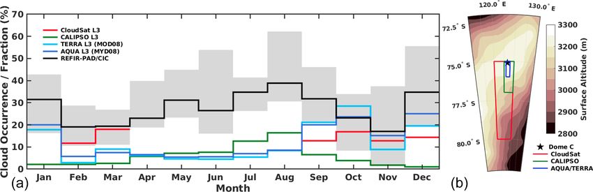
4.3 Monthly mean cloud occurrence: comparison with structed to provide completeness and consistency for the an-
satellite data ticipated users. These product types are frequently used to
perform climate analysis and model evaluation (e.g., Stuben-
CIC monthly mean cloud percentages (including ice and rauch et al., 2013; Webb et al., 2017). The assessment of
mixed-phase) for the period 2012–2015 are shown in Fig. 10 their accuracy can be particularly challenging, especially in
(left panel). The black curve corresponds to the 4-year remote regions such as the Antarctic Plateau, due to the
monthly average cloud occurrence, and the shaded gray area scarcity of ground-based stations that are available for prod-
indicates the minimum and maximum CIC monthly values. uct validation campaigns. For the present study, we only re-
The lowest average value is found in November (17 %), while fer to monthly mean L3 satellite products, and the compar-
higher occurrences are observed during the winter months. ison with CIC results is performed only in the context of
The peak is located in August, with an average value of 39 %. the objectives described above. A validation (that is outside
For the same month, the inter-annual variability is quite large, the scope of the present research) should be, eventually, per-
as indicated by the extent of the gray area. As examples, in formed on level 2 collocated satellite products to minimize
August the monthly mean values span from 31 % to 62 %, the bias due to different footprint sizes that can be otherwise
which is the highest derived occurrence, and in November very large when accounting for gridded L3 products. In prac-
from 1 % (lowest registered value) to 37 %. tice, different datasets present specific strengths and limita-
Monthly mean cloud occurrences and fractions derived tions that are briefly described below.
from level 3 (L3) satellite products are also reported in the The L3 products used in this work are derived from passive
left panel of Fig. 10 for the same period of time. The com- radiometric observations performed by the Moderate Res-
parison has a twofold objective: (a) to assess if the results olution Imaging Spectroradiometer (MODIS) on board the
obtained locally from the CIC/REFIR-PAD synergy can be TERRA and the AQUA satellite platforms, by the CALIOP
representative of the widespread region characterizing the on board the CALIPSO satellite, and by the CPR on board
Antarctic Plateau and (b) to estimate the differences among CloudSat satellite. For MODIS L3 products, the occurrence
the cloud occurrences and fractions derived from L3 satel- by cloud type is not available, and the cloud fraction is used.
lite products around the Concordia area. According to the This variable is computed as the ratio between the cloud-
WMO1 , the L3 satellite products are composed of variables covered pixels and the total number of pixels observed by
mapped on uniform space–time grid scales and are con- both satellite platforms each month and is mapped in a global
1 World Meteorological Organization – https://community.wmo.
grid of 1◦ of latitude and longitude, which corresponds to an
area of about 3000 km2 in the region of Concordia Station.
int/activity-areas/wmo-space-programme-wsp/data-products, last
In the right panel of Fig. 10 the boundary of the area which
access: 14 September 2021.
Atmos. Chem. Phys., 21, 13811–13833, 2021 https://doi.org/10.5194/acp-21-13811-2021You can also read