A Bayesian framework for emergent constraints: case studies of climate sensitivity with PMIP - CP
←
→
Page content transcription
If your browser does not render page correctly, please read the page content below
Clim. Past, 16, 1715–1735, 2020
https://doi.org/10.5194/cp-16-1715-2020
© Author(s) 2020. This work is distributed under
the Creative Commons Attribution 4.0 License.

A Bayesian framework for emergent constraints: case studies
of climate sensitivity with PMIP
Martin Renoult1 , James Douglas Annan2 , Julia Catherine Hargreaves2 , Navjit Sagoo1 , Clare Flynn1 ,
Marie-Luise Kapsch3 , Qiang Li4 , Gerrit Lohmann5 , Uwe Mikolajewicz3 , Rumi Ohgaito6 , Xiaoxu Shi5 , Qiong Zhang4 ,
and Thorsten Mauritsen1
1 Department  of Meteorology, Bolin Centre for Climate Research, Stockholm University, Stockholm, Sweden
2 Blue Skies Research Ltd, Settle, United Kingdom
3 Max Planck Institute for Meteorology, Hamburg, Germany
4 Department of Physical Geography, Bolin Centre for Climate Research, Stockholm University, Stockholm, Sweden
5 Alfred Wegener Institute, Helmholtz Centre for Polar and Marine Research, Bremerhaven, Germany
6 Japan Agency for Marine-Earth Science and Technology, Yokohama, Japan

Correspondence: Martin Renoult (martin.renoult@misu.su.se)

Received: 20 December 2019 – Discussion started: 17 January 2020
Revised: 4 July 2020 – Accepted: 27 July 2020 – Published: 10 September 2020

Abstract. In this paper we introduce a Bayesian frame-           tural uncertainty. The approach is compared with other ap-
work, which is explicit about prior assumptions, for using       proaches based on OLS, a Kalman filter method, and an al-
model ensembles and observations together to constrain fu-       ternative Bayesian method. An interesting implication of this
ture climate change. The emergent constraint approach has        work is that OLS-based emergent constraints on ECS gener-
seen broad application in recent years, including studies con-   ate tighter uncertainty estimates, in particular at the lower
straining the equilibrium climate sensitivity (ECS) using the    end, an artefact due to a flatter regression line in the case of
Last Glacial Maximum (LGM) and the mid-Pliocene Warm             lack of correlation. Although some fundamental challenges
Period (mPWP). Most of these studies were based on ordi-         related to the use of emergent constraints remain, this paper
nary least squares (OLS) fits between a variable of the cli-     provides a step towards a better foundation for their potential
mate state, such as tropical temperature, and climate sensi-     use in future probabilistic estimations of climate sensitivity.
tivity. Using our Bayesian method, and considering the LGM
and mPWP separately, we obtain values of ECS of 2.7 K
(0.6–5.2, 5th–95th percentiles) using the PMIP2, PMIP3, and
PMIP4 datasets for the LGM and 2.3 K (0.5–4.4) with the          1   Introduction
PlioMIP1 and PlioMIP2 datasets for the mPWP. Restricting
the ensembles to include only the most recent version of each    In recent years, researchers have identified a number of rela-
model, we obtain 2.7 K (0.7–5.2) using the LGM and 2.3 K         tionships between observational properties and a future cli-
(0.4–4.5) using the mPWP. An advantage of the Bayesian           mate change, which was not immediately obvious a priori but
framework is that it is possible to combine the two periods      which exists across the ensemble of global climate models
assuming they are independent, whereby we obtain a tighter       (GCMs) (Allen and Ingram, 2002; Hall and Qu, 2006; Boé
constraint of 2.5 K (0.8–4.0) using the restricted ensemble.     et al., 2009; Cox et al., 2018) participating in the Climate
We have explored the sensitivity to our assumptions in the       Model Intercomparison Project (CMIP). These relationships
method, including considering structural uncertainty, and in     are generally referred to as “emergent constraints” as they
the choice of models, and this leads to 95 % probability of      emerge from the ensemble behaviour as a whole rather than
climate sensitivity mostly below 5 K and only exceeding 6 K      from explicit physical analysis.
in a single and most uncertain case assuming a large struc-         Such emergent constraints have been broadly used to con-
                                                                 strain properties of the Earth’s climate system which are not

Published by Copernicus Publications on behalf of the European Geosciences Union.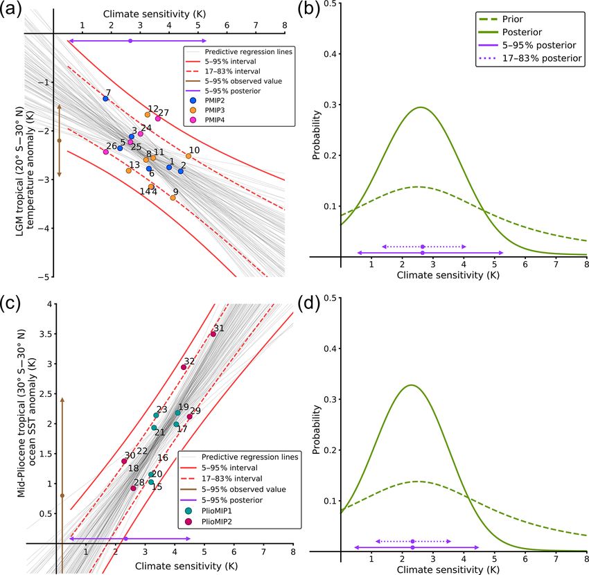
1716                                                       M. Renoult et al.: A Bayesian framework for emergent constraints

easily or directly observable. These are usually presented in     the climate system parameter(s) that we are primarily inter-
probabilistic terms, mostly based on ordinary least squares       ested in for this study, i.e. the climate sensitivity. Thus, their
(OLS) methods. For example, studies have explored the con-        prior predictive distribution for the climate system parameter
straint on equilibrium climate sensitivity (ECS), which is the    is not immediately clear and may not be so easily specified
global mean equilibrium temperature after a sustained dou-        as in the approach we explore here.
bling of CO2 over pre-industrial levels, using model out-            We present an alternative Bayesian linear regression ap-
puts from the Paleoclimate Model Intercomparison Project          proach in which the regression relationship is used as a like-
(PMIP) (Hargreaves et al., 2012; Schmidt et al., 2014;            lihood model for the problem. This allows the prior over the
Hopcroft and Valdes, 2015; Hargreaves and Annan, 2016).           predictand to be defined separately from and entirely inde-
Because of their relatively strong temperature signal, pale-      pendently of the model ensemble and emergent constraint
oclimate states like the Last Glacial Maximum (LGM) and           analysis. Thus, the likelihood arising from the emergent con-
the mid-Pliocene Warm Period (mPWP) are often considered          straint could be used to update a prior estimate of the predic-
to be promising constraints for the ECS (Hargreaves et al.,       tand that arose from a different source.
2012; Hargreaves and Annan, 2016), in particular at the high         In Sect. 2 we provide an overview of the concept of emer-
end.                                                              gent constraints, the previous methods used for these analy-
   Almost all emergent constraint studies have used OLS-          ses, the Bayesian framework, and the models and data em-
based methods to establish the link between variables in the      ployed in the paper. Section 3 describes the results, starting
model ensembles. However, whether ECS or another climate          with analysis of models and data from the Paleoclimate Inter-
parameter was investigated, the theoretical foundations for       comparison Project (PMIP) phases 2 and 3 for the LGM and
the calculations have not previously been clearly presented.      mPWP, which have previously been analysed for an emer-
An additional problem arising from this is the resulting dif-     gent constraint on climate sensitivity (Schmidt et al., 2014;
ficulty in synthesising estimates of climate system properties    Hargreaves and Annan, 2016). We then incorporate some
generated by different statistical methods with different, and    CMIP6 and PMIP4 model outputs that have been made avail-
often not explicitly introduced, assumptions. These methods       able to us for these periods to illustrate how these outputs fit
include OLS but also alternative Bayesian approaches such         into the same analysis. We also use the LGM and mPWP
as estimates of the climate sensitivity using energy balance      outputs to demonstrate how the method allows independent
models (Annan et al., 2011; Aldrin et al., 2012; Bodman and       emergent constraints to be combined. Finally, we discuss the
Jones, 2016).                                                     influences of the prior and model inadequacy on climate sen-
   Two recent papers have also addressed the question of          sitivity in Sect. 3.5 and 3.6, respectively.
emergent constraints in different ways. Bowman et al. (2018)
presented a hierarchical statistical framework which went a
long way to closing the gap in theoretical understanding of       2   Methods
emergent constraints. Conceptually, it is very similar to a
single-step Kalman filter, with which the iteration process       The general method of emergent constraints seeks a phys-
is avoided to only keep a single updating of a prior into a       ically plausible relationship in the climate system between
posterior. Specifically, it uses the model distribution approx-   two model variables in an ensemble of results from different
imated as a Gaussian as a prior, which is then updated using      climate models. Consequently, an observation of one mea-
the observation to a posterior. However, such a prior and the     surable variable (such as past tropical temperatures) could
underlying assumptions attached to it could be seen as a re-      be used to better constrain the other investigated variable,
strictive choice to impose on the climate sensitivity area of     usually unobserved and difficult to measure (such as cli-
research. In particular, most of the posterior values would       mate sensitivity). This idea has been used in climate science
lie in the range covered by the ensemble of models if the         to estimate quantities of interest such as snow albedo feed-
observed value is either uncertain and/or close to the prior      back (Hall and Qu, 2006), future sea ice extent (Boé et al.,
mean. This is a direct consequence of the joint probability       2009; Notz, 2015), low-level cloud feedback (Brient et al.,
distribution produced by the Kalman filter, which in the case     2016), and the equilibrium climate sensitivity (Hargreaves
of joint Gaussian distributions will produce a tighter poste-     et al., 2012; Schmidt et al., 2014; Cox et al., 2018). Although
rior Gaussian distribution. Because of that, it does not appear   the unobserved variable is usually taken as a future variable,
to correspond to the choice which is usually made, albeit im-     the emergent constraints theory can be used with two vari-
plicitly.                                                         ables within the same timeframe, as long as the relationship
   Another Bayesian statistical interpretation of emergent        is plausible. A summary of several different emergent con-
constraints has recently been presented by Williamson and         straints on climate sensitivity was made by Caldwell et al.
Sansom (2019), who extended the standard approach to ac-          (2018). This approach using emergent constraints is mean-
count for more general sources of uncertainty including           ingful only if we believe that reality satisfies the same re-
model inadequacy. A key aspect of their approach is that          lationship and it was not observed purely by chance in the
they set a prior on the observational constraint rather than      model ensemble. There is a risk in searching for such re-

Clim. Past, 16, 1715–1735, 2020                                                      https://doi.org/10.5194/cp-16-1715-2020
M. Renoult et al.: A Bayesian framework for emergent constraints                                                                    1717

lationships in a small ensemble that we may find examples              representation of the number of random intervals contain-
which are coincidental, with no real predictive value (Cald-           ing the true interval bounds (at 90 % confidence, this would
well et al., 2014). Spurious relationships could also be found         lead to 90 out of 100 random intervals containing the true
because of model limitations (Fasullo and Trenberth, 2012;             bounds), while the Bayesian credible interval is an interval
Grise et al., 2015; Notz, 2015).                                       which we believe (with the given probability) to contain the
   In this study, we focus on the relationship between equi-           truth. For instance, if there is an observed Ttropical = 1 K, with
librium climate sensitivity, defined here as S, and the tem-           an assumed Gaussian observational uncertainty of σ = 0.25
perature change in the tropics which is observed at the Last           at 1 standard deviation, then stating that there is a close-to-
Glacial Maximum (LGM) and the mid-Pliocene Warm Pe-                    95 % probability of having the true value of the parameter
riod (mPWP), defined as Ttropical . We posit that a relationship       within the interval 0.5–1.5 K is a Bayesian credible interval
between climate sensitivity and temperature change is physi-           interpretation. However, the latter is a common interpreta-
cally plausible, as we expect the long-term quasi-equilibrium          tion of frequentist-based studies. This confusion has inherent
temperature to be mainly influenced by radiative forcing, and          drawbacks for the analysis of posterior outputs, as shown in
in many model ensembles, variations in climate sensitivity             various fields of science (Hoekstra et al., 2014) and more re-
have been dominated by tropical feedbacks, mostly arising              cently for climate sensitivity computations (Annan and Har-
from low-level clouds (Bony et al., 2006; Vial et al., 2013).          greaves, 2020). Williamson and Sansom (2019) have pre-
                                                                       sented a Bayesian interpretation of this approach using refer-
2.1   Ordinary least squares                                           ence priors on ψ, as defined by Cox et al. (2018), as a met-
                                                                       ric of global mean temperature variability and the regression
The most widely used approach to emergent constraint anal-             coefficients. However, this approach does not appear to read-
ysis is to find an observable phenomenon that exhibits some            ily allow for the use of any arbitrary prior distribution for S,
relationship to the parameter of interest and use this as a pre-       which may either be desired for comparison with other re-
dictor in a linear regression framework. The ordinary least            search or have arisen through a previous unrelated analysis.
squares (OLS) method has been widely used because of its               The Bayesian linear regression approach that we introduce in
simplicity, so we also use it here as a starting point for com-        the next section avoids these problems.
parison with alternative statistical methods. In the context of
constraining climate sensitivity, the parameter of interest (i.e.
                                                                       2.2   Bayesian framework
the ECS) is considered to be a predicted variable (Hargreaves
et al., 2012; Schmidt et al., 2014; Hargreaves and Annan,              The (subjective) Bayesian paradigm is based on the premise
2016). This may be written as                                          that we use probability distributions to describe our uncer-
                                                                       tain beliefs concerning unknown parameters. We use Bayes’
S = γ × Ttropical + δ + ζ,                                      (1)    theorem to update a prior probability distribution function
where S is the climate sensitivity, γ and δ two unknown pa-            (PDF) for the equilibrium climate sensitivity via
rameters, Ttropical the temperature anomaly averaged over the
                                                                                               o
                                                                                      P Ttropical  |S P (S)
tropical region for the given paleo-time interval, and ζ the
                                                                               o
residual term which is drawn from a Gaussian distribution              P S|Ttropical   =                   ,                  (2)
                                                                                                  o
                                                                                              P Ttropical
N(0, σ 2 ) and which accounts for deviations from the linear
fit. When we use this approach, the unknown constants of the
                                                                                      o
                                                                       where P S|Ttropical       is the posterior estimate of S after con-
linear fit are estimated via ordinary least squares (OLS) us-
             i
ing the (Ttropical , S i ) pairs representing the model ensemble                                                       o
                                                                       ditioning on the geological proxy data Ttropical     , P (S) is the
(here i indexes the models), and then the equation is used to
                                                                                        o

predict the true value of S for the climate system based on            prior, and P Ttropical is a normalisation constant. The like-
                           o

the observed value Ttropical    . A confidence interval for the pre-                o
                                                                       lihood P Ttropical   |S is a function that takes any value of S
dictor variable can be generated by accounting for uncertain-          and generates a probabilistic prediction of what we would ex-
ties in the fit and in the observed value through a simulation                                 o
                                                                       pect to observe as Ttropical    if that value was correct. The use
of an ensemble of prediction as demonstrated by Hargreaves             of the Bayesian paradigm requires us to create such a func-
et al. (2012). This procedure makes the assumption that re-            tion. Using the principles of emergent constraint analyses in
ality satisfies the same regression relationship as the models,        which a linear relationship between these two parameters,
i.e. is likely to be at a similar distance from the line as the        which was seen in the GCM ensemble, is believed to also
model points are.                                                      apply to reality, it is natural to use the regression relationship
    Integrating the intrinsically frequentist confidence inter-
vals obtained from regression methods used for OLS esti-               Ttropical = α × S + β + ,                                     (3)
mates into a Bayesian framework is challenging. One issue
is the misinterpretation of frequentist confidence intervals           where α, β, and σ , the standard deviation of  as  ∼
as Bayesian posterior credible intervals. The former is the            N(0, σ 2 ), are three a priori unknown parameters. Note that

https://doi.org/10.5194/cp-16-1715-2020                                                             Clim. Past, 16, 1715–1735, 2020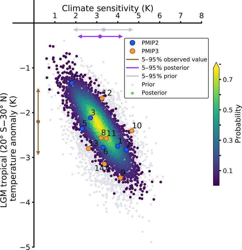
1718                                                         M. Renoult et al.: A Bayesian framework for emergent constraints

this reverses the roles of predictor and predictand compared        model ensemble, we can create a plausible likelihood model
to the OLS-based approach (Eq. 1). It implies that S is able to     for P (Ttropical |S).
give a prediction of Ttropical with a given uncertainty. This is       It is important to note that Eq. (3) and the conditioning of
physically plausible, as S is considered one of the best met-       parameters on the model ensemble only relate to the gener-
rics to represent temperature change. In particular, S is often     ation of the likelihood. The emergent constraint calculation
diagnosed in climate models from an abrupt and sustained            itself is then a second step thatuses this likelihood
                                                                                                                           to calcu-
quadrupling of CO2 from pre-industrial conditions (4xCO2 ),                                                 o
                                                                    late the posterior of interest P S|Ttropical   (Eq. 2). To apply
which usually leads to weak non-linearity similar to what is        the emergent constraints theory, it is required to insert a geo-
observed from LGM or mPWP climate dynamics. Therefore,                                      o
                                                                    logical observation Ttropical estimated through proxy data and
it is possible to use the 4xCO2 -computed S of climate mod-
                                                                                                  o
                                                                    obtain the likelihood P Ttropical |S , which leads to the pos-
els to predict Ttropical , assuming  as a representation of all
processes not related to S.

                                                                                     o
                                                                    terior P S|Ttropical    by Bayesian updating. We perform this
    Choosing S as the predictor (Eq. 3) will cause some dif-
ferences to the inference of the posterior S compared to the        step through a simple
                                                                                            importance sampling
                                                                                                                  algorithm by ap-
                                                                                                    o
                                                                    proximating P Ttropical = Ttropical  |S . That is, for any given
OLS-based approach introduced in Eq. (1). The plausibil-
ity of the existence of an emergent constraint between S            sensitivity S, we can calculate the probability of the obser-
and Ttropical is independent of the method chosen. Whether          vation of tropical temperature that we have as the compo-
Ttropical is a predicted or predictor variable, or whether the      sition of the predictive PDF for actual tropical temperature,
applied method uses OLS or Bayesian statistics, the meth-           together with the uncertainty associated with the observation
ods estimate different unknown parameters to investigate a          itself. The emergent constraint theory is thus applied with a
similar assumed relationship within the model ensemble, so          two-stage Bayesian process, including in first stage the BLR
it is expected that these different methods will yield similar      and in the second stage a Bayesian updating.
but not identical results. This was previously argued in the           A prior belief on climate sensitivity (P (S)) in the Bayesian
context of a hierarchical statistical model for emergent con-       updating process, and on the parameters of the regression
straints by Tingley et al. (2012). The Bayesian approach with       model in the BLR process, has to be assumed. There is no
S as the predictor is appropriate for emergent constraint anal-     clearly uncontested choice for prior distribution for climate
yses thanks to its transparency and handling of uncertainties.      sensitivity. However, Annan and Hargreaves (2011) argued
This has been explored by Sherwood et al. (2020) and is also        that a Cauchy distribution has a reasonable behaviour with a
investigated in this study. Thus, here we explore the imple-        long tail to high values but, unlike the uniform prior, does not
mentation of the Bayesian method for emergent constraint            assign high probability to these values. Thus, we adopt this
analyses for models and data that have already been investi-        prior for our main analyses. In Sect. 3.5 we test the sensitivity
gated with alternative methods (Hargreaves et al., 2012; Har-       of the results to this choice and compare the results obtained
greaves and Annan, 2016).                                           using gamma and uniform prior distributions. Priors for the
    The three parameters α, β, and σ in Eq. (3) are con-            parameters of the regression model are chosen with reference
ditioned on the model ensemble defined by its pairs of              to the specific experiment and are intended to represent our
    i
(Ttropical , S i ) (with i indexing the models). We estimate them   reasonable expectation that models do indeed generate a re-
via a Bayesian linear regression (BLR) procedure, which re-         gression relationship as described.
quires priors to be defined over these parameters. Conse-              An additional issue that was briefly mentioned above is
quently, the likelihood P (Ttropical |S) for a given S (as re-      that we may like to consider the probability that reality is
quired by Eq. 2) is an integration over the posterior distri-       qualitatively and quantitatively distinguishable from all mod-
bution of Ttropical predicted by the regression relation (con-      els. This issue, which was explicitly argued in the context
volved with observational uncertainty where appropriate)            of emergent constraint analysis by Williamson and Sansom
and conditioned on the model ensemble through α, β, and             (2019), seems reasonable since all models do share a the-
σ.                                                                  oretical heritage and certain limitations. However, this issue
    In this way, we create a statistical model that can gener-      remains challenging to quantify. It has not been considered in
ate a predictive PDF for the tropical temperature change at         most previous studies, which also makes it difficult to com-
the LGM or at the mPWP P (Ttropical |S) for any given sensi-        pare. We investigate this issue in Sect. 3.6. Whilst the pro-
tivity. There is a structural difference between this approach      posed resolution remains preliminary and although the con-
and that of Eq. (1) in that here the residual uncertainties         cept is promising for understanding emergent constraints, we
 ∼ N(0, σ 2 ) represent our inability to perfectly predict the     decide to omit it for the bulk of our analysis to enable more
tropical temperature anomaly arising from a given sensitiv-         direct comparisons with previous studies.
ity and are probabilistically independent of the latter rather         The Bayesian method is more explicit than the standard
than the former variable. The issue here is not a matter of         OLS approach, as the prior assumptions have to be given by
which regression line is “correct”, but rather how, given the       the user. This transparency leads to more freedom and control

Clim. Past, 16, 1715–1735, 2020                                                        https://doi.org/10.5194/cp-16-1715-2020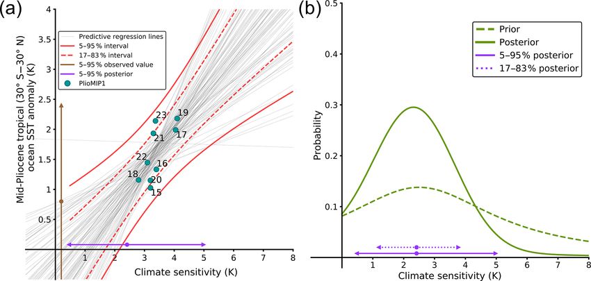
M. Renoult et al.: A Bayesian framework for emergent constraints                                                             1719

of the statistical model. Moreover, it has a reduced sensitivity   Pa = (I − KH)Pf ,                                           (6)
to outliers as the prior on the regression coefficients provides
a form of regularisation. This should lead to lower variance       where x is the mean, P its covariance, z the observations with
in the results compared to results with wider priors on the        an associated observational uncertainty covariance matrix R,
parameters, particularly with small model ensembles.               and H the operator that maps the model state onto observa-
   Additionally, the Bayesian method allows the user to add        tions. The superscripts f and a by convention refer to the fore-
multiple lines of evidence by updating the chosen prior for        cast (i.e. the prior in this work) and analysis (the posterior),
S. The method for combining independent constraints is rea-        respectively. While in many applications, such as numerical
sonably simple, as it only requires us to calculate and store      weather prediction, this method is applied in an iterative fash-
the posterior of the first emergent constraint analysed and use    ion with the analysis being used as the starting point of the
this distribution as the prior for the second emergent con-        next forecast, here it is only applied once as a way of imple-
straint. Thus, it is a direct form of sequential Bayesian up-      menting Bayesian updating to our prior in order to generate
dating. This process results in a posterior distribution which     the posterior.
will generally be narrower than either of the two posteriors          Here we only have two dimensions for the Gaussian, these
that would have been generated from either of the emergent         being the scalar predictor (e.g. sensitivity) and predictand
constraints separately. Although it may be tempting to simply      (e.g. tropical temperature change). While this approach is a
combine all emergent constraints in this way, it is necessary      natural and attractive option in many respects, it has the spe-
to also consider possible dependencies between the uncer-          cific drawback (in the context of this work) of using the dis-
tainties in the different emergent constraints before this can     tribution of model samples as a prior (for both the mean and
be done with confidence (Annan and Hargreaves, 2017).              covariance). Existing literature on emergent constraints does
   It is not clear if observational errors have always been ad-    not make this assumption, and this could be seen as a limiting
equately accounted for in previous emergent constraints re-        aspect of the method, as it implies that the model ensemble
search. Our approach provides a natural framework for this,        is already a credible predictor even before consideration of
as the likelihood can include the uncertainty of the observa-      the observational constraint. An implication of this approach
tional process as we have done. Recent studies have inves-         is that the posterior estimate will be equal to the model dis-
tigated Bayesian ways of integrating uncertainties on proxy        tribution in the case that no observational constraint exists,
reconstructions into the global temperature field (e.g. Tier-      either because there is in fact no relationship between the
ney et al., 2019). For the sake of comparison with Hargreaves      observation and predictand or when the observational un-
et al. (2012), Schmidt et al. (2014), and Hargreaves and An-       certainty is excessively large. The use of a Gaussian prior
nan (2016), we use the reconstructions and observational er-       based on the ensemble range also means that it is difficult for
rors adopted in these studies, which are based on multiple lin-    the method to generate posterior estimates that include val-
ear regressions and model–proxy cross-validation. However,         ues significantly outside the model range, even in the case
we have ignored uncertainties in the calculation of the model      in which the observed value is outside the model spread. We
values of S and Ttropical as, while they are poorly quantified,    present results generated with a Kalman filter in Sect. 3.1 for
we believe them to be too small to materially affect our re-       comparison with our main analysis.
sult. In fact, it has been argued for the case of the mPWP that
observational errors on S and Ttropical are small compared to      2.4   Climate models and data
the structural differences responsible of the dispersion of the
points around the regression line and can thus be neglected        The Bayesian method may be applied to any emergent con-
(Hargreaves and Annan, 2016).                                      straint. In this study, we use the model outputs and data syn-
                                                                   theses that have arisen from phases 2 and 3 of PMIP (Bra-
                                                                   connot et al., 2007; Haywood et al., 2011; Harrison et al.,
2.3   Kalman filter
                                                                   2014), as well as the few available models of phase 4 (Hay-
Bowman et al. (2018) recently presented a new interpretation       wood et al., 2016; Kageyama et al., 2017), summarised in
of emergent constraint analysis. Their framework is essen-         Table 1. The Last Glacial Maximum (19–23 ka) corresponds
tially a two-dimensional ensemble Kalman filtering approach        to the period of the last ice age when ice sheets and sea ice
in which the prior, represented by the model ensemble, is up-      had their maximum extent. Due to its temporal proximity,
dated according to the observation using the Kalman equa-          relative abundance of proxy data, and substantial radiative
tions, which approximate all distributions by a multivariate       forcing anomaly, the LGM is widely considered one of the
Gaussian (Kalman, 1960). The Kalman equations are given            best paleoclimate intervals for testing global climate models
by                                                                 and has been featured in all of the PMIP consortium exper-
                                                                   iments. A representation of several model LGM simulations
                        −1
                                                                   compared to the surface air temperature (SAT) reconstruction

K = Pf HT HPf HT + R        ,                               (4)
                                                                 of Annan and Hargreaves (2013) is shown in Fig. 1a.
x a = x f + K z − Hx f ,                                    (5)

https://doi.org/10.5194/cp-16-1715-2020                                                       Clim. Past, 16, 1715–1735, 2020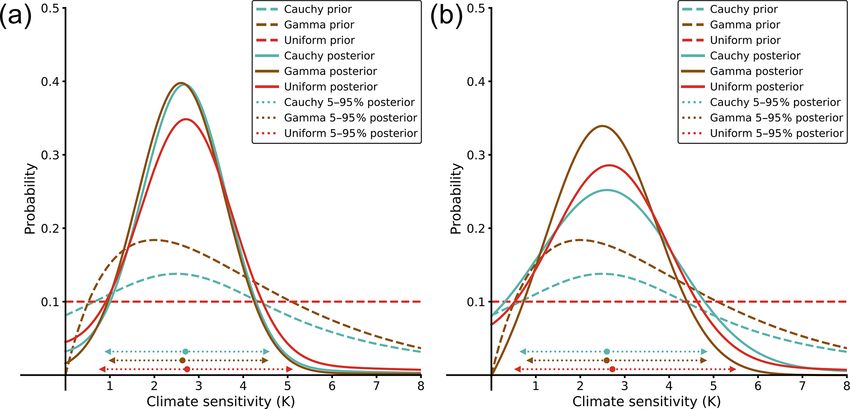
1720                                                                            M. Renoult et al.: A Bayesian framework for emergent constraints

Table 1. Models, tropical temperature (Ttropical ) outputs, and climate sensitivity (S) used in this study.

   Experiment                              Figure       Model                           a
                                                                                      Ttropical         S     S reference
                                        reference
   PMIP2 LGM                                      1     MIROC                           −2.75         4.0     K-1 Model Developers (2004)
   PMIP2 LGM                                      2     IPSL                            −2.83         4.4     Randall et al. (2007)
   PMIP2 LGM                                      3     CCSM                            −2.12         2.7     Randall et al. (2007)
   PMIP2 LGM                                      4     ECHAM                           −3.16         3.4     Randall et al. (2007)
   PMIP2 LGM                                      5     FGOALS                          −2.36         2.3     Randall et al. (2007)
   PMIP2 LGM                                      6     HadCM3b                         −2.77         3.3     Randall et al. (2007)
   PMIP2 LGM                                      7     ECBILTb                         −1.34         1.8     Goosse et al. (2005)
   PMIP3/CMIP5 LGM                               8      CCSM4b                           −2.6        3.2      Andrews et al. (2012)
   PMIP3/CMIP5 LGM                               9      IPSL-CM5A-LRb                   −3.38       4.13      Andrews et al. (2012)
   PMIP3/CMIP5 LGM                              10      MIROC-ESM                       −2.52       4.67      Sueyoshi et al. (2013)
   PMIP3/CMIP5 LGM                              11      MPI-ESM-P                       −2.56       3.45      Andrews et al. (2012)
   PMIP3/CMIP5 LGM                              12      CNRM-CM5b                       −1.67       3.25      Andrews et al. (2012)
   PMIP3/CMIP5 LGM                              13      MRI-CGCM3b                      −2.82        2.6      Andrews et al. (2012)
   PMIP3/CMIP5 LGM                              14      FGOALS-g2b                      −3.15       3.37      Masa Yoshimori, personal communication, 2013c
   PMIP4/CMIP6 LGM                              24      MPI-ESM1.2-LRb                  −2.06       3.01      Mauritsen et al. (2019)
   PMIP4/CMIP6 LGM                              25      MIROC-ES2Lb                     −2.23       2.66      Hajima et al. (2020), Ohgaito et al. (2020)
   PMIP4/CMIP6 LGM                              26      INM-CM4-8b                      −2.43       1.81      This study
   PMIP4/CMIP6 LGM                              27      AWI-ESM-1-1-LRb                 −1.75       3.61      This study
   PMIP3/CMIP5 PlioMIP1                         15      CCSM4b                            1.03       3.2      Haywood et al. (2013)
   PMIP3/CMIP5 PlioMIP1                         16      IPSLCM5A                          1.33       3.4      Haywood et al. (2013)
   PMIP3/CMIP5 PlioMIP1                         17      MIROC4mb                          1.99      4.05      Haywood et al. (2013)
   PMIP3/CMIP5 PlioMIP1                         18      GISS ModelE2-R                    1.16       2.8      Haywood et al. (2013)
   PMIP3/CMIP5 PlioMIP1                         19      COSMOSb                           2.18       4.1      Haywood et al. (2013)
   PMIP3/CMIP5 PlioMIP1                         20      MRI-CGCM2.3b                      1.15       3.2      Haywood et al. (2013)
   PMIP3/CMIP5 PlioMIP1                         21      HadCM3b                           1.93       3.3      Randall et al. (2007)
   PMIP3/CMIP5 PlioMIP1                         22      NorESM-L                          1.45       2.1      Haywood et al. (2013)
   PMIP3/CMIP5 PlioMIP1                         23      FGOALS-g2b                        2.14      3.37      Masa Yoshimori, personal communication, 2013c
   PMIP4/CMIP6 PlioMIP2                         28      GISS-E2-1-Gb                      0.92       2.6      This study
   PMIP4/CMIP6 PlioMIP2                         29      IPSL-CM6A-LRb                     2.12       4.5      This study
   PMIP4/CMIP6 PlioMIP2                         30      NorESM1-Fb                        1.37      2.29      Guo et al. (2019)
   PMIP4/CMIP6 PlioMIP2                         31      CESM2b                             3.5       5.3      Gettelman et al. (2019)
   PMIP4/CMIP6 PlioMIP2                         32      EC-EARTH3.3b                      2.94       4.3      Wyser et al. (2020)
 a For the LGM simulations (generations PMIP2, PMIP3, and PMIP4), the tropical average was defined between 20◦ S and 30◦ N (Hargreaves et al., 2012). For the mPWP
 simulations (generations PlioMIP1 and PlioMIP2), the tropical average was defined between 30◦ S and 30◦ N (Hargreaves and Annan, 2016). All temperature values are defined
 as changes compared to pre-industrial values. b Latest version of a model that was kept for the approach described in Sect. 3.3. c Calculated using the Gregory method on
 150 years of output, making it consistent with the values of Andrews et al. (2012).

   Previous results from PMIP2 showed a significant corre-                                  pilations are presently in development as part of PMIP4, but
lation between LGM tropical temperatures and climate sen-                                   these have yet to be integrated into a global temperature field,
sitivity in the models (Hargreaves et al., 2012), although the                              so revising the temperature estimate from Annan and Harg-
equivalent calculation for the PMIP3 models found no signif-                                reaves (2013) is a topic for future work.
icant correlation (Schmidt et al., 2014; Hopcroft and Valdes,                                  Interest in the mPWP (2.97–3.29 million years ago) as
2015). These two similar-sized ensembles with contrasting                                   a more direct analogy for future climate change has grown
characteristics are a good test bed for exploring the prop-                                 during the past years. This is the most recent period with
erties of the different methods. For the tropical temperature                               a sustained high level of greenhouse gases and concomi-
anomaly relative to the pre-industrial value we use a value                                 tant warmth relative to the pre-industrial period; however,
from Annan and Hargreaves (2013): for 20◦ S to 30◦ N a                                      the data are more sparse and uncertain. In Fig. 1b, the sea-
  o
Ttropical of −2.2 K with a Gaussian observational uncertainty                               surface temperature (SST) anomaly of different climate mod-
of ±0.7 K (5 %–95 % confidence interval). Several data com-                                 els which performed a mPWP simulation is displayed, as is

Clim. Past, 16, 1715–1735, 2020                                                                                      https://doi.org/10.5194/cp-16-1715-2020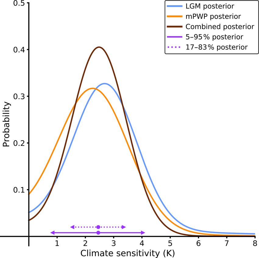
M. Renoult et al.: A Bayesian framework for emergent constraints                                                                     1721

Figure 1. Latitudinal distribution of temperature changes relative to pre-industrial values for both simulated climates for various climate
models and a proxy reconstruction. Dashed lines are models of the CMIP5 generation, while solid lines are models from the CMIP6 gener-
ation. All model distributions correspond to 100-year zonal averages when possible; certain CMIP5 PlioMIP1 models were averaged over
30 years. (a) SAT change of the LGM. The solid black line is a multi-proxy ensemble reconstruction taken from Annan and Hargreaves
(2013). (b) SST change of the mPWP. The solid black line is the multi-proxy ensemble reconstruction PRISM3 described by Dowsett et al.
(2009).

the PRISM3 SST reconstruction (Dowsett et al., 2009). Pre-              tion and Synoptic Mapping) SST anomaly field as described
vious results for this period from the Pliocene Model Inter-            in Dowsett et al. (2009).
comparison Project (PlioMIP) experiment, which was part                    The Last Interglacial (127 ka, referred to as lig127k in
of PMIP3, indicated a fairly strong correlation between trop-           CMIP6) and the mid-Holocene (6 ka) are part of the PMIP
ical temperature and climate sensitivity in the models, but the         simulations and also relatively warm climates. The forcings
confidence with which this can be used to constrain climate             are, however, seasonal and regional in nature, mostly influ-
sensitivity was low due to high uncertainty in various obser-           encing the patterns of climate change. The global change
vationally derived components and various compromises in                in temperature and the global climate forcing are both very
the way the protocol was formulated (Hargreaves and An-                 small, and this coupled with the large uncertainty in paleo-
nan, 2016). For the mPWP, a tropical temperature anomaly                climate data makes these intervals poor candidates for con-
of 0.8 ± 1.6 K (5 %–95 % interval) is taken from Hargreaves             straining climate sensitivity. We do not explore these inter-
and Annan (2016) for 30◦ S to 30◦ N, assuming the largest               vals further here.
5 %–95 % uncertainty shown in that work. The reconstruc-                   Climate sensitivity has various definitions and there are
tion used here is the PRISM3 (Pliocene Research, Interpreta-            also a number of different ways of approximating the value
                                                                        in climate models that have not been run to equilibrium. For

https://doi.org/10.5194/cp-16-1715-2020                                                             Clim. Past, 16, 1715–1735, 2020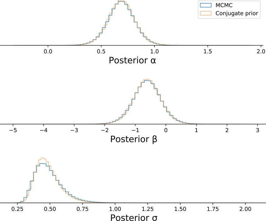
1722                                                       M. Renoult et al.: A Bayesian framework for emergent constraints

PMIP3 LGM the model values are mostly based on the re-            package spBayes (Finley et al., 2013, 2014), described in Ap-
gression method of Gregory et al. (2004), but for the mod-        pendix A, and leads to similar results.
els which contributed to PMIP2 LGM and PlioMIP the exact             Depending on the strength of the correlation among the
definition and derivation used in each case are not always        dataset, one could expect a sensitivity of the regression to the
clear in the literature. In order to make comparisons with        choice of prior parameters. In the following sections, we first
previous work, here we use the same values as those used          describe the physical arguments behind the choice of priors
in Hargreaves et al. (2012), Schmidt et al. (2014), and Harg-     over α, β, and σ and then present the outputs of the BLR
reaves and Annan (2016) with two exceptions to ensure that        for both the PMIP2 and PMIP3 dataset of the LGM and the
only one value of sensitivity is used for identical versions      PlioMIP1 dataset of the mPWP. Then, we include the CMIP6
of the same model across different experiments. Specifically,     data in the Bayesian framework for both paleo-intervals and
for FGOALS-g2 we use the value of 3.37 K (Masa Yoshi-             present an approach of combining the two emergent con-
mori, personal communication, 2013) for both PMIP3 LGM            straints. Finally, we explore the sensitivity of the Bayesian
and PMIP3 PlioMIP, and for HadCM3 we use 3.3 K (Ran-              approach to the choice of priors over the climate parameter
dall et al., 2007) for both PMIP2 LGM and PMIP3 PlioMIP.          of choice (i.e. the climate sensitivity) and to the hypothetical
Previous values used by Hargreaves and Annan (2016) for           inadequacy of climate models.
PMIP3 PlioMIP were 3.7 K for FGOALS-g2 (Zheng et al.,
2013) and 3.1 K for HadCM3 (Haywood et al., 2013). These          3.1   The Last Glacial Maximum
changes are minor compared to the ensemble range of cli-
mate sensitivity, and thus they have no significant effect on     From consideration of energy balance arguments and funda-
the posterior outputs.                                            mental physical properties, such as the response of the Earth
   In addition to the already published results from PMIP2        to an increase in CO2 , we have a prior expectation of a rela-
and PMIP3 we add to our ensembles the results that are cur-       tionship between sensitivity and the global LGM temperature
rently available from PMIP4 in Sect. 3.3. While the LGM           anomaly (e.g. Lorius et al., 1990), and the model experiments
protocol (Kageyama et al., 2017) remains very similar to that     of Hargreaves et al. (2007) and simple physical arguments
in previous iterations of PMIP, the mPWP protocol (Hay-           about the spatial distribution of forcing suggest that this re-
wood et al., 2016) has more significant differences which ad-     lationship may be most clearly visible when we focus on the
dress several of the limitations of the previous version. Most    tropical region. While the total negative forcing at the LGM
importantly, PlioMIP2 seeks to represent a specific quasi-        is roughly twice as large as the positive forcing that would
equilibrium climate state in the past rather than represent-      be caused by a doubling of CO2 , the temperature response at
ing an amalgamation of different warm peak climates as had        low latitudes is generally expected to be lower than the global
been the case for PlioMIP1. A priori we are therefore less        mean due to polar amplification and the related presence of
confident about combining the results from PlioMIP1 and           high-latitude ice sheets. Thus, we might reasonably expect
PlioMIP2 and do so mostly to indicate where the new models        the tropical temperature change at the LGM to be roughly
lie in the ensemble and to highlight the potential for future     equal to the global temperature rise under a doubling of CO2 .
research in this area once more model results based on the        It would also be unexpected if the correlation had the oppo-
PlioMIP2 protocol become available.                               site sign to that based on simple energy balance arguments
                                                                  such that a more sensitive model had a lower temperature
                                                                  change at the LGM. However, we cannot justify imposing a
3   Applications and results                                      precise constraint on the slope and therefore our choice of
                                                                  prior for α is N (−1, 12 ). As for β, we expect the regression
In order to apply the Bayesian linear regression and com-         line to pass close to the origin, as a model with no sensitiv-
pute the likelihood P (Ttropical |S), several priors have to be   ity to CO2 would probably have little response to any other
established as initial conditions. Specifically, for both the     forcing changes, especially in the tropical region where the
LGM and the mPWP we use Eq. (3) as the basis for our              influence of ice sheets is remote. However, we do not expect
likelihood function. The prior expectations of the three un-      a precise fit to the origin, and therefore the prior chosen for
known parameters α, β, and the standard deviation of the          β is N(0, 12 ). Finally, we chose a wide prior for σ , a half-
residual , referred to as σ , need to be defined. The relative   Cauchy with a scale parameter of 5. The Cauchy is fairly
complexity of the likelihood function with three a priori un-     close to uniform for values smaller than the scale parameter,
known parameters requires the use of a sampling method for        decaying gradually for higher values.
computational efficiency. In this study, we use the Markov           Deviations from the regression line may be due to dif-
chain Monte Carlo (MCMC) method NUTS as described                 ferent efficacies of other forcing components, especially ice
by Hoffman and Gelman (2014). The NUTS method is also             sheets or dust. To take into account the uncertainty on the
included in the MCMC Python package PyMC3 (Salvatier              strength of the response, we performed two additional anal-
et al., 2016), which is applied here. The approach is alter-      yses wherein the prior response was smaller (α defined as
natively described as a conjugate prior problem using the R       N(−0.5, 12 )) and larger (α defined as N(−2, 12 )). We do not

Clim. Past, 16, 1715–1735, 2020                                                      https://doi.org/10.5194/cp-16-1715-2020
M. Renoult et al.: A Bayesian framework for emergent constraints 1723
Table 2. Summary of the methods and computed posterior sensitivities; n/a indicates “not applicable”.
Experiment Method∗ 5 %–95 % 5 %–95 % Median 5 %–95 %
prior (K) o
Ttropical (K) (K) posterior (K)
LGM PMIP2 BF Cauchy prior 0.5–28.7 −2.9 to −1.5 2.7 1.0–4.5
LGM PMIP2 BF gamma prior 0.7–9.5 −2.9 to −1.5 2.6 1.0–4.5
LGM PMIP2 BF uniform prior 0.5–9.5 −2.9 to −1.5 2.7 0.8–5.0
LGM PMIP2 OLS predicted CS n/a −2.9 to −1.5 2.8 1.0–4.5
LGM PMIP2 Kalman filter 1.7–4.5 −2.9 to −1.5 2.9 1.8–4.1
LGM PMIP2 BF α prior mean = −2 0.5–28.7 −2.9 to −1.5 2.7 1.0–4.4
LGM PMIP2 BF α prior mean = −0.5 0.5–28.7 −2.9 to −1.5 2.7 0.9–4.6
LGM PMIP2+PMIP3 BF Cauchy prior 0.5–28.7 −2.9 to −1.5 2.6 0.7–4.8
LGM PMIP2+PMIP3 BF gamma prior 0.7–9.5 −2.9 to −1.5 2.6 0.9–4.8
LGM PMIP2+PMIP3 BF uniform prior 0.5–9.5 −2.9 to −1.5 2.7 0.6–5.4
LGM PMIP2+PMIP3 OLS predicted CS n/a −2.9 to −1.5 3.0 1.4–4.6
LGM PMIP2+PMIP3 Kalman filter 2.0–4.5 −2.9 to −1.5 3.2 2.2–4.2
LGM PMIP2+PMIP3 BF α prior mean = −2 0.5–28.7 −2.9 to −1.5 2.6 0.8–4.7
LGM PMIP2+PMIP3 BF α prior mean = −0.5 0.5–28.7 −2.9 to −1.5 2.6 0.7–4.8
LGM PMIP2+PMIP3 BF model inadequacy 0.5–28.7 −2.9 to −1.5 2.8 0.5–5.8
LGM PMIP3 BF Cauchy prior 0.5–28.7 −2.9 to −1.5 2.8 0.7–5.5
LGM PMIP3 OLS predicted CS n/a −2.9 to −1.5 3.4 1.3–5.6
LGM PMIP2+PMIP3+PMIP4 BF Cauchy prior 0.5–28.7 −2.9 to −1.5 2.7 0.6–5.2
LGM “latest” models BF Cauchy prior 0.5–28.7 −2.9 to −1.5 2.7 0.7–5.2
LGM “latest” models BF model inadequacy 0.5–28.7 −2.9 to −1.5 2.8 0.5–6.3
mPWP PlioMIP1 BF Cauchy prior 0.5–28.7 −0.8 to 2.4 2.4 0.5–5.0
mPWP PlioMIP1 BF α prior mean = 2 0.5–28.7 −0.8 to 2.4 2.4 0.5–4.8
mPWP PlioMIP1 BF α prior mean = 0.5 0.5–28.7 −0.8 to 2.4 2.4 0.5–5.1
mPWP PlioMIP1 BF model inadequacy 0.5–28.7 −0.8 to 2.4 2.5 0.5–5.4
mPWP PlioMIP1+PlioMIP2 BF Cauchy prior 0.5–28.7 −0.8 to 2.4 2.3 0.5–4.4
mPWP “latest” models BF Cauchy prior 0.5–28.7 −0.8 to 2.4 2.3 0.4–4.5
mPWP “latest” models BF model inadequacy 0.5–28.7 −0.8 to 2.4 2.4 0.4–5.0
mPWP and LGM, “latest” models BF Cauchy prior 0.5–28.7 −2.9 to −1.5 2.5 0.8–4.0
mPWP and LGM, with CMIP6 BF Cauchy prior 0.5–28.7 −2.9 to −1.5 2.4 0.7–4.1
∗ BF: Bayesian framework. OLS: predictive range via ordinary least squares. Truncated-at-zero Cauchy prior: peak: 2.5, scale: 3. Gamma prior: peak: 2,
scale: 2. Uniform prior: bounded 0–10. The “latest” model ensembles are those created from the most recent versions of each model (see Sect. 3.3).
see much difference in the results using the three priors over allowing for a substantial probability of having high climate
α: the difference is approximately 0.2 K of climate sensitiv- sensitivity while still maintaining some preference for more
ity for both the upper and lower percentiles quoted, giving us moderate values. However, the sensitivity of Bayesian statis-
confidence in our choice of N(−1, 12 ). The computed 5 %– tics to the choice of prior has often been noted. Thus, two al-
95 % posterior climate sensitivity ranges for different values ternative priors, including the widely used uniform prior, and
of α are summarised in Table 2. their corresponding posterior distributions are investigated in
The MCMC algorithm samples the posterior distribution Sect. 3.5.
of regression parameters, which is represented by the ensem- To test the robustness of the method and also to compare
ble of predictive regression lines in Fig. 2. This ensemble it with the statistical methods used in previous studies, three
is used to infer the climate sensitivity following the Bayesian cases are investigated in which we use different combinations
inference approach using the geological reconstruction of the of the available model ensembles. The results are shown in
LGM tropical temperature. The posterior distributions of S Fig. 2 and Table 2.
are computed using a truncated-at-zero Cauchy prior with a For the PMIP2 ensemble, the correlation between tropi-
peak of 2.5 and a scale of 3, which corresponds to a wide cal temperature and climate sensitivity was found to be rea-
5 %–95 % prior interval of 0.5–28.7 K. Such a prior was used sonably strong, and in this study the resulting 5 %–95 %
previously by Annan et al. (2011) because it has a long tail, range for inferred climate sensitivity is 1.0–4.5 K (Fig. 2b).
https://doi.org/10.5194/cp-16-1715-2020 Clim. Past, 16, 1715–1735, 20201724 M. Renoult et al.: A Bayesian framework for emergent constraints Figure 2. LGM northern tropical (20◦ S–30◦ N) temperature versus climate sensitivity for the PMIP2 and PMIP3 models. (a, c, e) Predictive regression lines sampled with the MCMC method. (b, d, f) Corresponding posterior climate sensitivity computed with a Cauchy prior and inferred from a geological reconstruction taken from Hargreaves et al. (2012). (a, b) Analysis done on the PMIP2 dataset; (c, d) analysis done on the PMIP2 and PMIP3 combined dataset; (e, f) analysis done on the PMIP3 dataset. The numbers on each point refer to the models used as listed in Table 1. Clim. Past, 16, 1715–1735, 2020 https://doi.org/10.5194/cp-16-1715-2020
M. Renoult et al.: A Bayesian framework for emergent constraints                                                                   1725

The range is slightly better constrained at the lower end
than the 0.5–4 K from Hargreaves et al. (2012); however, we
have used the revised value for the LGM tropical anomaly
of −2.2 ± 0.7 K rather than the value of −1.8 ± 0.7 K that
was used by Hargreaves et al. (2012). The Bayesian-inferred
value is similar to the OLS-inferred method with the revised
version (Table 2), giving confidence in the proximity of both
methods in the case of high correlation.
   When all the models of PMIP2 and PMIP3 (see Ta-
ble 1) were considered jointly the correlation became weaker
and the corresponding 5 %–95 % range generated by the
Bayesian method is 0.7–4.8 K (Fig. 2d). Schmidt et al. (2014)
obtained 1.6–4.5 K using a similar ensemble although in that
case multiple results obtained from the same modelling cen-
tre were combined by averaging. Using the OLS method on
our ensemble and generating predicted values, we obtain a
5 %–95 % range of 1.4–4.6 K. The Bayesian method gener-
ates a wider range here, particularly at the lower end, as the
correlation is weaker and the prior starts to influence the pos-
terior.
   Finally, we consider the PMIP3 models in isolation. For
                                                                     Figure 3. LGM northern tropical (20◦ S–30◦ N) temperature versus
this ensemble no correlation is found, so for the Bayesian
                                                                     climate sensitivity of the PMIP2 and PMIP3 models. The Kalman
method the result is heavily dependent on our prior as-              filtering is applied to the ensemble of both PMIP2 and PMIP3. The
sumptions. We obtain a 5 %–95 % range here of 0.7–5.5 K              numbers on each point refer to the models used as listed in Table 1.
(Fig. 2f). Applying the OLS-based prediction method to the
PMIP3 dataset gives a 5 %–95 % range of 1.3–5.6 K. As pre-
viously argued for the combination of PMIP2 and PMIP3, the
                                                                     pared to our Bayesian linear regression method. However,
latter method produces a tighter posterior range at the lower
                                                                     this is strongly forced by the underlying assumptions of a
end. In the absence of a correlation, the Bayesian method
                                                                     Kalman filter (Sect. 2.3), which uses the model ensemble as
relaxes to the prior, whereas the predictions obtained via
                                                                     a prior, making it difficult to compute a posterior range out-
the OLS method are heavily influenced by the range of the
                                                                     side the model range, in particular when the observed value is
ensemble. Additionally, as previously argued in Sect. 2.2,
                                                                     considered excessively uncertain. Thus, although the Kalman
the differences in the posterior 5 %–95 % range between the
                                                                     filtering method could be interesting, we do not consider it
Bayesian and OLS-based approaches are partly connected to
                                                                     further, as we stipulate that its assumptions are too restric-
choosing S as a predictor or predicted, respectively. The im-
                                                                     tive for the question of emergent constraints, and it therefore
pact of such choice will be even bigger as the correlation
                                                                     cannot be a relevant method in its current form to efficiently
gets weaker, since the difference between the respective er-
                                                                     assess S and, in particular, its uncertainty.
ror parameters  and ζ will increase. However, we emphasise
that this does not suggest that either range is closer to reality.
Although the comparison between methods with a predictor             3.2   The mid-Pliocene Warm Period
or predicted S should get more complex from a philosophi-
cal point of view as  differs from ζ , we stipulate that both       As for the LGM, prior parameters have to be defined to per-
ranges can be considered valuable information regarding S            form the BLR with the mPWP data. In principle these may
within a climate and emergent constraint framework.                  be different to those used for the LGM experiment, since the
   The Kalman filtering approach presented by Bowman                 total positive forcing of the mPWP is not as large as the neg-
et al. (2018) has not previously been used for emergent con-         ative forcing of the LGM, but in practice we have adopted
straint analyses in paleoclimate research. Thus, we also use         the same priors for our base case, apart from the obvious sign
this method to explore both PMIP2 and the combination of             change for α. We performed the same sensitivity experiments
PMIP2 and PMIP3 (Fig. 3). With the same geological re-               as for the LGM, with three different priors over α: N (1, 12 ),
construction value and a prior 5 %–95 % range (based on the          N (0.5, 12 ), and N(2, 12 ). There was only a small difference
PMIP2 GCM ensemble) of 1.7–4.5 K, a posterior range of               between the results using the three priors: the differences at
S of 1.8–4.1 K is inferred. By combining the PMIP2 and               the 5th percentile were less than 0.1 K, and the differences at
PMIP3 models, the prior 5 %–95 % range becomes 2.0–4.5 K             the 95th percentile were approximately 0.3 K (see Table 2).
and the posterior range is 2.2–4.2 K. The increase in the            Regarding β and σ , there is no physical reason for their pri-
lower bound in these calculations is the largest change com-         ors to be substantially different than the ones chosen for the

https://doi.org/10.5194/cp-16-1715-2020                                                           Clim. Past, 16, 1715–1735, 2020
1726 M. Renoult et al.: A Bayesian framework for emergent constraints
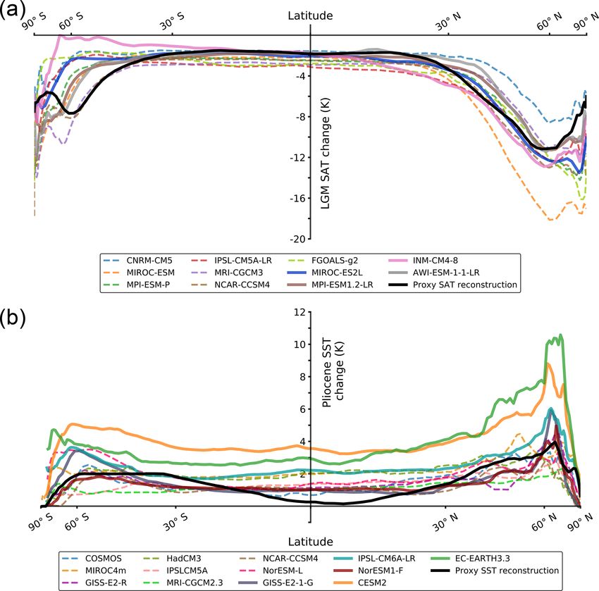
Figure 4. The mPWP tropical (30◦ S–30◦ N) temperature versus climate sensitivity of the PlioMIP1 models. (a) Predictive regression
lines sampled with an MCMC method. (b) Corresponding posterior climate sensitivity computed with a Cauchy prior and inferred from a
geological reconstruction taken from Dowsett et al. (2009). The numbers on each point refer to the models used as listed in Table 1.
LGM. Thus, a N(0, 12 ) prior for β is selected, and the same although we believe such dependencies exist in the ensem-
prior for σ as for the LGM analysis is chosen. ble, it is in reality difficult to quantify and correct for this.
The Bayesian inference method applied above for the How to deal with this possible duplication of information is
LGM model outputs is now applied to the mPWP model therefore a subjective decision. In Schmidt et al. (2014) it
outputs (Fig. 4). With less abundant models and less well- was taken into account by averaging the results from mod-
constrained temperature data, we prefer to assume large un- els from the same modelling centre. Here we take an alter-
certainties in the mPWP SST reconstruction (0.8 ± 1.6 K, native approach of including only the latest version of each
5 %–95 % confidence). We adopt the Cauchy prior on climate model. This gives an ensemble size of 11 models (Table 2)
sensitivity as for the LGM analysis (5 %–95 % interval of and a 5 %–95 % climate sensitivity range of 0.7–5.2 K with
0.5–28.7 K) and compute a 5 %–95 % interval for the ECS of the Bayesian method. The range here is relatively wide and
0.5–5.0 K for the PlioMIP1 dataset. Similar to the results for close to the range computed with the ensemble of PMIP2,
the LGM, the predictions via the OLS method (Hargreaves PMIP3, and PMIP4. This is due to the removal of almost
and Annan, 2016) resulted in a slightly narrower 5 %–95 % all PMIP2 models in this restricted ensemble, which leaves
range than the Bayesian method (1.3–4.2 K, assuming 1.6 K mainly the poorly correlated PMIP3 ensemble and the en-
of uncertainty on the data). semble of PMIP4 together.
For PlioMIP1 and PlioMIP2 the situation is a little more
complex as the protocol has been redesigned to represent a
3.3 Inclusion of CMIP6 and PMIP4 data specific interglacial state rather than a generic warm climate,
referred to as a “time slab” in the PlioMIP protocol. Thus,
The ongoing PMIP4 experiments have produced LGM and
there could be a different regression relationship for these
mPWP (PlioMIP2) simulations. Here we add those results to
two ensembles. However, when we plot the PlioMIP1 ensem-
our ensembles. There are four model runs available for the
ble members (Fig. 5d) we see that they do not look different
LGM and five for the mPWP (see Table 2) on 1 May 2020.
to the PlioMIP2 ensemble members. The straight combina-
For the LGM we have previously combined the PMIP2
tion of PlioMIP1 and PlioMIP2 gives an ensemble range of
and PMIP3 results, and the protocol for PMIP4 is not very
14 models and we computed a 5 %–95 % range of 0.5–4.4 K.
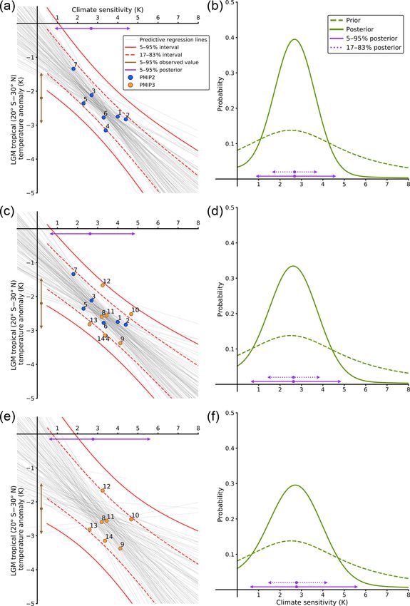
different. If we combine all three ensembles we obtain a
Including only the most recent versions of models results in
5 %–95 % range for the ECS of 0.6–5.2 K using the Bayesian
an ensemble size of 11 models (Table 2) and generates a
method (Fig. 5b). The ensemble size is now 18, but we note
nearly identical 5 %–95 % climate sensitivity range of 0.4–
that this includes several models coming from the same mod-
4.5 K with the mPWP simulation. Thus, for this period the
elling centres. Past studies have investigated the proximity
inclusion of the PlioMIP2 models allows for a tighter con-
of models with hierarchical trees (Masson and Knutti, 2011;
straint at the upper bound, much aided by the larger spread
Knutti et al., 2013) and the influence of their dependency
of S in these new models.
on statistical methods (Annan and Hargreaves, 2017). Thus,
Clim. Past, 16, 1715–1735, 2020 https://doi.org/10.5194/cp-16-1715-2020M. Renoult et al.: A Bayesian framework for emergent constraints 1727
Figure 5. Inclusion of the CMIP6 models into the Bayesian method for the LGM and the mPWP. (a) LGM northern tropical (20◦ S–30◦ N)
temperature versus climate sensitivity of the PMIP2, PMIP3, and PMIP4 models and (b) inferred climate sensitivity. (c) The mPWP tropical
(30◦ S–30◦ N) temperature versus climate sensitivity of the PlioMIP1 and PlioMIP2 models and (d) inferred climate sensitivity. For both
inferences, the prior used is a Cauchy distribution defined with a peak of 2.5 and a scale of 3. The numbers on each point refer to the models
used as listed in Table 1.
3.4 Combining multiple constraints model experiments. Moreover, modelling uncertainties that
influence the regression analysis are expected to arise from
As described in Sect. 2.4, the mPWP and the LGM are very rather different sources, such as the response to ice sheets and
different climates. If the observational data are generated a cold climate in one case versus the influence of a warmer
by unrelated analyses, we may be able to consider the two climate in the other. Having said that, model biases influ-
lines of evidence to be independent and combine them using encing the simulation of one climate change may also in-
Bayes’ theorem to create a new posterior which is likely to fluence the other, which means that if similar models occur
be narrower than that arising from either analysis alone. As- in both ensembles, this could lead to dependencies. Using
suming that the uncertainties arising from the mPWP and the Bayes’ theorem to combine the constraints means that it is
LGM analyses are independent of each other may be plau- not necessary for the same set of models to be used for each
sible as the proxy reconstructions use different observations ensemble, but, as we can see from Table 1, a few models do
and analyses to estimate both the tropical temperatures and occur in both ensembles.
the other variables that act as boundary conditions for the
https://doi.org/10.5194/cp-16-1715-2020 Clim. Past, 16, 1715–1735, 2020You can also read