Seasonal variation of the sound-scattering zooplankton vertical distribution in the oxygen-deficient waters of the NE Black Sea - Ocean Science
←
→
Page content transcription
If your browser does not render page correctly, please read the page content below
Ocean Sci., 17, 953–974, 2021
https://doi.org/10.5194/os-17-953-2021
© Author(s) 2021. This work is distributed under
the Creative Commons Attribution 4.0 License.

Seasonal variation of the sound-scattering zooplankton vertical
distribution in the oxygen-deficient waters of the NE Black Sea
Alexander G. Ostrovskii, Elena G. Arashkevich, Vladimir A. Solovyev, and Dmitry A. Shvoev
Shirshov Institute of Oceanology, Russian Academy of Sciences, 36, Nakhimovsky prospekt, Moscow, 117997, Russia

Correspondence: Alexander G. Ostrovskii (osasha@ocean.ru)

Received: 10 November 2020 – Discussion started: 8 December 2020
Revised: 22 June 2021 – Accepted: 23 June 2021 – Published: 23 July 2021

Abstract. At the northeastern Black Sea research site, obser-     layers is important for understanding biogeochemical pro-
vations from 2010–2020 allowed us to study the dynamics           cesses in oxygen-deficient waters.
and evolution of the vertical distribution of mesozooplank-
ton in oxygen-deficient conditions via analysis of sound-
scattering layers associated with dominant zooplankton ag-
gregations. The data were obtained with profiler mooring and      1   Introduction
zooplankton net sampling. The profiler was equipped with an
acoustic Doppler current meter, a conductivity–temperature–       The main distinguishing feature of the Black Sea environ-
depth probe, and fast sensors for the concentration of dis-       ment is its oxygen stratification with an oxygenated upper
solved oxygen [O2 ]. The acoustic instrument conducted ul-        layer 80–200 m thick and the underlying waters contain-
trasound (2 MHz) backscatter measurements at three angles         ing hydrogen sulfide (Andrusov, 1890; see also review by
while being carried by the profiler through the oxic zone. For    Oguz et al., 2006). Early studies of the oxic zone indicated
the lower part of the oxycline and the hypoxic zone, the nor-     that the vertical distribution of zooplankton hinges on oxy-
malized data of three acoustic beams (directional acoustic        gen stratification (Nikitin, 1926; Petipa et al., 1960). Later,
backscatter ratios, R) indicated sound-scattering mesozoo-        the dives of the manned research submersible Argus showed
plankton aggregations, which were defined by zooplankton          that the zooplankton vertical distribution was not uniform
taxonomic and quantitative characteristics based on strati-       (Vinogradov et al. 1985; Flint 1989). In particular, the thin-
fied net sampling at the mooring site. The time series of         layered structure of zooplankton distribution was observed
∼ 14 000 R profiles as a function of [O2 ] at depths where        by the Argus research pilot in the lower part of the oxic
[O2 ] < 200 µm were analyzed to determine month-to-month          zone. Thereafter, zooplankton sampling with a vertical res-
variations of the sound-scattering layers. From spring to         olution of 3–5 m using a 150 L sampler with an attached
early autumn, there were two sound-scattering maxima cor-         conductivity–temperature–depth (CTD) probe indicated that
responding to (1) daytime aggregations, mainly formed by          the daytime deep aggregations of the zooplankton popula-
diel-vertical-migrating copepods Calanus euxinus and Pseu-        tions were associated with layers of certain water density
docalanus elongatus and chaetognaths Parasagitta setosa,          (Vinogradov and Nalbandov, 1990; Vinogradov et al., 1992).
usually at [O2 ] = 15–100 µm, and (2) a persistent monospe-       The deeper zooplankton aggregation was formed by the fifth
cific layer of the diapausing fifth copepodite stages of C. eu-   copepodite stage of Calanus ponticus (former name of C. eu-
xinus in the suboxic zone at 3 µm < [O2 ] < 10 µm. From late      xinus), and its lower boundary was at the specific density
autumn to early winter, no persistent deep sound-scattering       surface σ2 = 15.9, where the oxygen concentration was ap-
layer was observed. At the end of winter, the acoustic            proximately 4 µm. The diapausing cohort of C. ponticus did
backscatter was basically uniform in the lower part of the        not perform vertical migrations and occupied the suboxic
oxycline and the hypoxic zone. The assessment of the sea-         layer around the clock (Vinogradov et al., 1992). The ac-
sonal variability of the sound-scattering mesozooplankton         cumulation of a high lipid reserve, a decrease in the rate
                                                                  of oxygen consumption, and a delay in gonad development

Published by Copernicus Publications on behalf of the European Geosciences Union.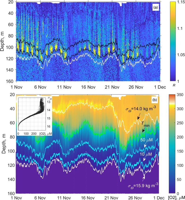
954                  A. G. Ostrovskii et al.: Seasonal variation of the sound-scattering zooplankton vertical distribution

were defined as characteristic features of diapausing C. eu-        – above the hydrogen sulfide zone in the suboxic
xinus (Vinogradov et al., 1992; Arashkevich et al., 1998;             layer (where the concentration of dissolved oxygen
Svetlichny et al., 2002, 2006). The vertically migrating zoo-         [O2 ] < 10 µm (Murray et al., 1989, Oguz et al., 2006)
plankters (ctenophores Pleurobrachia pileus, chaetognaths             and above that, in the oxycline ([O2 ] increases from
Parasagitta setosa, and older copepodites of Pseudocalanus            10 to 280–300 µm with decreasing depth), where sound
elongatus and C. euxinus) formed daytime aggregations be-             scattering occurs from both suspended particles and
tween isopycnals 15.7–15.5 and 15.4–14.9 and at an oxygen             mesozooplankton with characteristic sizes from 200 µm
concentration of 11–40 µm. At night, the migrant zooplank-            to 20 mm;
ters inhabited the upper layers and peaked in the thermocline
(Vinogradov et al., 1985). The descent of zooplankters into         – above the oxycline in the oxygen-rich euphotic zone,
the hypoxic zone during the daytime may give an energetic             where large-cell phytoplankton (Yunev et al., 2020) be-
advantage to migrating specimens due to a decrease in the             come an additional sound-scattering agent.
rate of oxygen consumption and locomotor activity at low
oxygen concentrations, as has been shown for females of               Using a combination of ultrasound sensing and stratified
C. euxinus (Svetlichny et al., 2000). This and other experi-      zooplankton sampling was necessary to resolve the ocean
mental studies contributed to the development of an optimal       fine-scale vertical distribution of mesozooplankton. An anal-
behavioral strategy model (Morozov et al., 2019) for struc-       ysis of both echograms and simultaneous stratified net sam-
tured populations of two species, C. euxinus and P. elon-         pling showed that the SSLs at 2 MHz were associated with
gatus. The authors parameterized the model using seasonal         the zooplankton species C. euxinus and P. elongatus at
field observations in the NE Black Sea and showed that the        σ2 = 15.7–15.4 and diapausing C. euxinus above σ2 = 15.9
diel vertical migrations of these species could be explained as   (Arashkevich et al., 2013).
the result of a trade-off between depth-dependent metabolic           The specific theme of this study is the seasonal change in
costs, anoxia, available food, and predation.                     the sound-scattering zooplankton vertical distribution across
   Zooplankton aggregations result in sound-scattering layers     the oxygen gradient from the lower part of oxygenated wa-
(SSLs). Diel vertical migration was observed using ship echo      ter to the anoxic zone boundary. This theme is in line with
sounding at frequencies of 120–200 kHz (Erkan and Gücü,           the EU Horizon 2020 BRIDGE-BS project (https://cordis.
1998; Mutlu, 2003, 2006, 2007; Stefanova and Marinova,            europa.eu/project/id/101000240, last access: 19 July 2021),
2015). The diurnal dynamics of C. euxinus and chaetog-            which focuses on Black Sea ecosystem functioning. While
naths were documented from shipborne echograms (Mutlu             the project relies on future observations and methods for un-
2003, 2006). The lower boundary of the migrating C. eux-          derstanding biogeochemical processes at several pilot sites,
inus was defined as σ2 = 16.15–16.2 for the daytime, and          this paper presents ongoing observations at the northeastern
the migrating chaetognaths were defined as σ2 = 15.9–16.0         Black Sea Gelendzhik site. The acoustic data were collected
(Mutlu 2007). In July 2013, a multifrequency (38, 120, and        year-round and analyzed to infer the SSL seasonal variabil-
200 kHz) shipborne echo-sounder survey over the southern          ity in relation to the oxygen stratification. Our observational
Black Sea revealed that the daytime deep distribution of mi-      study was made possible using a moored Aqualog profiler,
grating C. euxinus was bounded by σ2 values between 15.2          equipped with an ultrasound probe, a CTD probe, and a fast
and 15.9 (Sakınan and Gücü, 2016). In the above studies, the      oxygen sensor. The advantage of this approach is that it pro-
persistent layer of diapausing C. euxinus was not detected in     vides frequent year-round measurements (with an interval of
the echograms.                                                    up to 1 h) of collocated vertical profiles of sound scattering,
   The 24 h rhythm in the pattern of sound scattering was         temperature, salinity, and dissolved oxygen concentration in
a prominent feature of the 2 MHz acoustic sensing data ob-        the water column from the near surface to the bottom layer
tained by a moored profiler station (Ostrovskii and Zatsepin,     with a high vertical resolution (up to 20 cm). This helps to
2011) in the NE Black Sea. The data obtained by a short           fill in the gaps due to insufficient zooplankton sampling in
(up to 10 d) experimental deployment of a moored automatic        the winter season and resolves difficulties with sampling at
mobile profiler, equipped with an ultrasound probe operat-        precise depths, thereby providing the information needed to
ing at a frequency of 2 MHz and a dissolved oxygen sensor,        define the displacements of the mesozooplankton aggrega-
allowed Ostrovskii and Zatsepin (2011) to define the main         tions.
sound-scattering zones as follows:                                    The goals of the analysis are as follows: (1) to develop
                                                                  methods to visualize the SSLs in the lower part of the oxy-
                                                                  cline and in the hypoxic zone, (2) to validate the SSLs in the
  – the hydrogen sulfide zone below the specific density          oxygen-deficient waters using the taxonomic and quantita-
    surface σ2 = 15.9–16.0 (Yakushev et al., 2005), where         tive characteristics of zooplankton vertical distribution de-
    sound is scattered by sedimented detritus and mineral         rived from stratified net sampling, and (3) to describe the
    particles, whose fluxes vary temporally while being           seasonal variations of the deep mesozooplankton SSLs, in-
    rather homogeneous at different depths;                       cluding the diapause duration of CV C. euxinus, in relation

Ocean Sci., 17, 953–974, 2021                                                         https://doi.org/10.5194/os-17-953-2021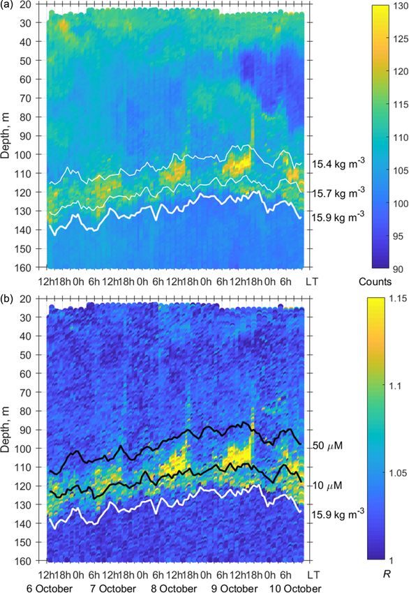
A. G. Ostrovskii et al.: Seasonal variation of the sound-scattering zooplankton vertical distribution                        955

to oxygen concentration (the oxygen bounds for the meso-         contribution to the average value is made by the scattering in
zooplankton SSLs).                                               the center of the measurement cell at a distance of approxi-
                                                                 mately 1.1 m from the transducer. The device can transmit
                                                                 up to 23 sound pulses every 1 s. The average value of the
2   Measurements                                                 volume scattering strength for sound pulses transmitted and
                                                                 received in 1 s is recorded in the device’s memory.
This study is based on the comparative analysis of the am-          The high frequency of 2 MHz allows for observations of
plitude of sound backscattering data at a frequency of 2 MHz     small-sized sound scatterers. Theoretically, a 2 MHz trans-
and oxygen concentration data in seawater obtained in the        ducer is most sensitive to particles with a diameter of
NE Black Sea using a moored automatic mobile profiler,           0.23 mm (estimates for different frequencies for standard
Aqualog (Fig. 1) (Ostrovskii and Zatsepin, 2011, 2016; Os-       seawater are given, for example, in Hofmann and Peeters,
trovskii et al., 2013). To obtain the depth profiles of the      2013). However, this is not entirely applicable to zooplank-
volume backscattering strength, the Aqualog profiler was         ton due to the complex shape of these organisms, their struc-
equipped with a Nortek Aquadopp acoustic Doppler cur-            ture, their lipid composition, and the presence of gases in
rent meter (https://www.nortekgroup.com/assets/documents/        their bodies (Stanton et al., 1994; Lavery et al., 2007; Law-
ComprehensiveManual_Oct2017_compressed.pdf, last ac-             son et al., 2006). However, as a simplified model, copepod
cess: 19 July 2021).                                             species are often considered cylinders, the scattering from
   The Aquadopp is a narrow-band instrument                      which is defined as a function of the incident sound pres-
(https://support.nortekgroup.com/hc/en-us/articles/              sure, the acoustic wavelength, and the distance between the
360029839331-The-Comprehensive-Manual-ADCP,                      transmitter and the animal. An approximate formula for de-
last access: 19 July 2021) that emits short sound pulses         scribing sound scattering from an elongated weakly scatter-
(pings) at a constant frequency and receives reflected (echo)    ing body of an animal also includes the angle of orienta-
signals. Plankton and suspended matter, as well as air and       tion of the body (Stanton et al., 1993, 1994). Unfortunately,
gas bubbles, are the main scatterers of the sound. While         the manufacturer of the Aquadopp instrument does not spec-
sound pulses are scattered in all directions when they           ify information about the acoustic power of its transducers.
hit particles, a small fraction of the incident sound pulse      The Aquadopp measurement data for the volume scattering
intensity is reflected. The Aquadopp current meter employs       strength are presented in conventional units (counts). With-
a mono-static system in which three transducers are used         out special calibration, it is not possible to determine the
to transmit and receive signals at an acoustic frequency of      amount of falling sound pressure in water at a distance from
2 MHz. Measurements are made in the 90 dB range with a           the instrument transducer.
resolution of 0.45 dB. In high-accuracy acoustic Doppler            Since 2013, Aquadopp instruments with sideways-looking
measurements, the acoustic beams are narrow, and each            vertically mounted heads have been regularly used on the
has a cone angle of 1.7◦ . Three focused beams measure           Aqualog profiling carrier (Fig. 1). The carrier moves up or
the scattering strength with high sampling rates in a small      down at a speed of approximately 0.2 m s−1 , so the verti-
volume (referred to as a single point). Two-sided acoustic       cal resolution of the volume scattering strength data is 0.2 m.
beams are directed horizontally with 90◦ spacing between         These data are averaged every 5 s, allowing for the detection
the axes of the beams (Fig. 1). These beams measure the          of an SSL with a thickness on the order of 1 m.
volume scattering strength at the level of the transducer.          In the context of this study, the ability to observe sound
The third beam is inclined at an angle of 45◦ to the plane       that has been reflected from zooplankton species at differ-
formed by the axes of the other two beams. The piezoelectric     ent angles is important. In the case of settling detritus, the
element of the transducer transmits sound waves when it          volume scattering strength of slanted beam A3 and that of
vibrates. The vibration does not stop at once but is damped      horizontal beams A1 or A2 are approximately the same. If
over time. The speed of sound in water and the damping time      the elongated suspended particles are oriented vertically or
of the membrane vibration determine the dead zone. In our        inclined, the amplitude of A3 will significantly differ from
case, this distance along the acoustic beam is approximately     the amplitudes of A1 and A2 . This was shown for copepods
0.35 m from the piezoelectric element of the transducer          based on both models of acoustic scattering at a frequency of
to the measurement cell (in the form of a truncated cone).       2 MHz (Stanton and Chu, 2000; Roberts and Jaffe, 2007) and
The sound pulses are scattered and reflected back to the         laboratory experiments (Roberts and Jaffe, 2008).
transducer. In our case, the length of the cell along the axis      Thus, by comparing the amplitudes A1 , A2 , and A3 , one
of the acoustic beam is approximately 1.5 m. Therefore, the      can judge the predominant orientation of species in zoo-
reflected sound pulse intensity obtained by the instrument       plankton aggregations. It is assumed that the aggregation’s
is the weight average for the time during which the sound        characteristic size is greater than the length of the acoustic
wave passes the distance of 1.85 m to the far boundary of        measurement cell, that is, not less than ∼ 2 m, and its lifetime
the measurement cell plus 1.85 m on the way back. The            is longer than 10 s. Therefore, during the Aqualog carrier
received signal is processed in such a way that the greatest     movement at a speed of 0.2 m s−1 , the slanted and horizontal

https://doi.org/10.5194/os-17-953-2021                                                         Ocean Sci., 17, 953–974, 2021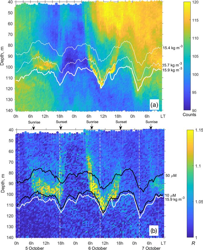
956                   A. G. Ostrovskii et al.: Seasonal variation of the sound-scattering zooplankton vertical distribution

Figure 1. The moored Aqualog automatic mobile profiler with a deep-water Aquadopp acoustic Doppler current meter (a). Transducer head
of the shallow-water Aquadopp acoustic Doppler current meter on the Aqualog profiler (b). Bottom right: the acoustic beams are shown in
blue and are labeled A1 , A2 , and A3 .

acoustic beams scan the same zooplankton aggregation. The                In addition to the Aquadopp instrument, a SeaBird 52MP
complexity and variability of the acoustic backscatter makes          CTD probe and Aanderaa 4330F and SBE 43F dissolved
it difficult to compare the acoustic signals obtained for dif-        oxygen fast sensors were incorporated into the Aqualog
ferent observational periods. Proper normalization of the sig-        profiler aerobic zone (Ostrovskii and Zatsepin, 2016). The
nals is needed to evaluate the seasonal change in the vertical        SeaBird 52MP CTD was specially designed for a moored
distribution of the mesozooplankton SSLs from many pro-               profiling application in which the instrument makes vertical
files despite the variability of the amplitude of the acoustic        profile measurements from a carrier that travels verti-
backscatter. For the Aquadopp instrument, such normaliza-             cally beneath a subsurface floatation (https://www.seabird.
tion is the ratio of the volume scattering strength of the hori-      com/sbe-52-mp-moored-profiler-ctd-optional-do-sensor/
zontal beams to the volume scattering strength of the slanted         product-downloads?id=60762467706,           last      access:
beam:                                                                 19 July 2021). The CTD is equipped with a pump that
                                                                      controls a flow at a constant speed through a single small
R = (A1 + A2 )/2A3 .                                         (1)
                                                                      diameter opening to ensure the minimization of salinity
   It allows for a drastic reduction in the noise associated with     spiking in the measurement data by the temperature and
clouds of sinking particles, which have an approximately              conductivity cell. On the Aqualog profiling carrier slowly
equal area in the horizontal projection to the projection with        moving at ∼ 0.2 m s−1 , the CTD sampling rate of once per
a 45◦ angle of inclination. In some cases, the suspended              second provides sufficient data to resolve ocean fine-scale
particles can completely obscure the signal associated with           thermohaline structure. The accuracy of the CTD probe
the aggregation of mesozooplankton. However, in this study,           is 0.002 ◦ C for the temperature, ± 0.0003 S m−1 for the
there were usually only a few such cases. As will be shown            conductivity, and ± 0.1 % of the full scale range for the
below in Sect. 3, typically at depths from 60 to 120 m during         pressure. The SBE 43F accuracy should be no worse than
the day, the directional acoustic backscatter ratio R = 1.05–         ± 2 % saturation, which can be compared with 5 % for
1.2, and at night, R < 1.05. In the Appendix, we will con-            Aanderaa 4330F with a resolution better than 1 µm or 0.4 %
sider whether the mesozooplankton specimens’ vertical ori-            (https://www.aanderaa.com/media/pdfs/d378_aanderaa_
entation is tilted in the deep aggregations. The analysis will        oxygen_sensor_4330_4330f.pdf, last access: 19 July 2021).
be based on calculation of the ratio of the volume scattering         In practice, in the Black Sea, SBE 43F showed very robust
strength of the horizontal beams A1 /A2 , assuming that due           results in detecting the lower boundary of the oxic zone,
to the tilt the standard deviation of A1 /A2 should be greater        consistent with observations of the sigma-density structure
than 0.                                                               and definition of the oxic zone boundary for the northeastern

Ocean Sci., 17, 953–974, 2021                                                              https://doi.org/10.5194/os-17-953-2021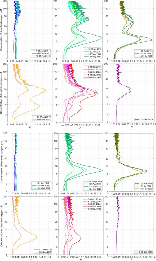
A. G. Ostrovskii et al.: Seasonal variation of the sound-scattering zooplankton vertical distribution                           957

                                                                       To acquire taxonomic and quantitative features of zoo-
                                                                    plankton vertical distribution, stratified net samples were
                                                                    taken from R/V Ashamba (Table 1) near the moored pro-
                                                                    filer Aqualog with a Juday net (mouth area 0.1 m2 , mesh size
                                                                    180 µm) equipped with a closing device. The towing speed
                                                                    was 0.9–1.0 m s−1 , and the net was closed without stopping
                                                                    the upward movement. The sampling was carried out in calm
                                                                    weather so that the wire angle was not higher than 10◦ . The
                                                                    sampling was carried out at earlier stages of this project in
                                                                    June 2010, October 2013, and July 2014, as well as later in
                                                                    October 2016.
                                                                       The net hauls targeted the backscattering aggregation con-
                                                                    sidering that their locations were associated with specific
                                                                    isopycnal layers (Ostrovskii and Zatsepin, 2011, Fig. 9). Ver-
Figure 2. The Black Sea coastline (https://osmdata.openstreetmap.   tical profiles of temperature, salinity, and density were ob-
de/data/coastlines.html, last access: 19 July 2021). The observa-   tained with a shipborne SeaBird 19plus CTD probe prior to
tional site off Gelendzhik is shown by a red dot. © OpenStreetMap   mesozooplankton sampling. Depth strata were chosen based
contributors 2021. Distributed under the Open Data Commons          on the CTD profiles to sample the upper mixed layer (UML),
Open Database License (ODbL) v1.0.                                  the thermocline layer, the layer from the oxycline upper
                                                                    boundary (σ2 = 14.25) to the lower boundary of the thermo-
                                                                    cline, and two layers in the oxygen-deficient zone: the layer
region of the Sea (Ostrovskii and Zatsepin, 2016). The
                                                                    from depths of σ2 15.7 to σ2 15.4 and the layer from 2–3 m
SeaBird 52MP CTD with SBE 43F was regularly calibrated
                                                                    below σ2 15.9 to σ2 15.7.
at the facility of the Southern Branch of the Shirshov
                                                                       The time of sampling corresponded to the day–night
Institute of Oceanology, Gelendzhik. The dissolved oxygen
                                                                    vertical distribution and upward–downward migration of
measurements using the Aanderaa 4330F and SBE 43F
                                                                    zooplankton (June 2010), the daytime distribution (Octo-
sensors at the profiler were described in Ostrovskii and
                                                                    ber 2013), and the day–night distribution (July 2014 and
Zatsepin (2016) and later in a companion paper (Ostrovskii
                                                                    October 2016). The samples were immediately fixed with
et al., 2018). The fast-response sensing foils of the Aanderaa
                                                                    buffered formaldehyde (4 % final concentration of seawater–
4330F sensor were replaced by new foils two times in
                                                                    formaldehyde solution). The volume of filtered sea water was
the past 4 years. The CTD and dissolved oxygen sensors
                                                                    estimated from the area of the net mouth and the length of the
were mounted at the leading edge of the Aqualog profiler
                                                                    released wire. Organisms were identified and counted under a
pointing into horizontal oncoming flow, while hydrodynamic
                                                                    stereomicroscope equipped with an ocular micrometer. Zoo-
cowling (vertically oriented, wing-like) helped to stabilize
                                                                    plankters were identified at the level of species and age stages
the profiler orientation with respect to the flow direction.
                                                                    of copepods and size classes (with an interval of 2 mm)
It should be noted that the Black Sea environment is par-
                                                                    of chaetognaths and ctenophores. The smallest organisms
ticularly suitable for profiling measurements since there is
                                                                    (meroplankton, appendicularians, copepod nauplii, and ova)
no biological fouling on the sensors of the profiler, which
                                                                    considered in the analysis were 180 µm in size. Mesozoo-
is usually submerged into the hydrogen sulfide zone for
                                                                    plankton biomass in terms of dry weight (DW) was estimated
∼ 10 min every 1–2 h. Finally, the dissolved oxygen sensor
                                                                    based on the published length–DW regressions for different
data were verified with the water samples at standard depths
                                                                    species summarized in Arashkevich et al. (2014, Table 2).
for determination of dissolved oxygen by Winkler method
                                                                    Biomass values were standardized to units of milligrams of
(not shown here).
                                                                    dry weight per cubic meter (mg DW m−3 ) or milligrams of
   The profiler mooring station was deployed approximately
                                                                    dry weight per square meter (mg DW m−2 ). The intensity of
4 nmi from the coast at the uppermost part of the continental
                                                                    the echo signal strongly depends on the material properties of
slope at 44◦ 29.30 N and 37◦ 58.70 (Fig. 2). From June 2010 to
                                                                    the organism’s tissue (Stanton et al., 1994); therefore, when
April 2021, 16 surveys lasting from a few days to 3 months
                                                                    comparing the pattern of the scattering signal intensity with
were carried out (Table 1) (Solovyev et al., 2021). During the
                                                                    the pattern of zooplankton distribution in a community con-
surveys, the device automatically performed a profiling cycle
                                                                    taining different taxa, it was reasonable to express zooplank-
usually every 1–2 h, descending to the near-bottom depth of
                                                                    ton biomass as DW or carbon (Flagg and Smith, 1989; Hey-
200–220 m and ascending to the upper layer while remain-
                                                                    wood et al., 1991; Ashjian et al., 1998). For a graphical pre-
ing submerged at a depth of 20–40 m. In particular, in 2016–
                                                                    sentation of the results, six components of zooplankton were
2020, more than 14 000 multiparameter sets of vertical pro-
                                                                    considered: copepods Calanus euxinus and Pseudocalanus
files were collected year-round (except March).
                                                                    elongatus, small crustaceans (Acartia clausi, Paracalanus
                                                                    parvus, Oithona similis and cladocerans), heterotrophic di-

https://doi.org/10.5194/os-17-953-2021                                                            Ocean Sci., 17, 953–974, 2021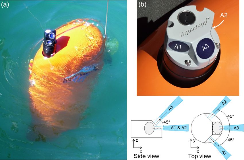
958                           A. G. Ostrovskii et al.: Seasonal variation of the sound-scattering zooplankton vertical distribution

Table 1. Deployments of the profiler Aqualog-6 with a Nortek Aquadopp current meter in the NE Black Sea and the dates of the zooplankton
sampling near the profiler mooring site in 2010–2021. Since 2013, the profiler Aqualog has been equipped with a SBE 52MP CTD probe
with a SBE 43F DO sensor. Additional sensors used on the profiler were as follows: Oxygen Aanderaa 4330F, Seapoint Turbidity Meter, and
Seapoint Fluorometer. The unit “cpd” denotes the profiling cycles per day.

  Survey       Start (UTC)                End (UTC)           Profile        Profile    Number        Additional sen-   Stratified net sampling for zoo-
                                                              cycle          depth      of profiles   sors at           plankton/sampling for determi-
                                                              interval, h    range, m                 the profiler      nation of dissolved oxygen by
                                                                                                                        Winkler method
  1            21 Jun 2010 16:03          22 Jun 2010 16:50              1     19–245           25    a                 Zooplankton:
                                                                                                                        21 Jun 2010 18:05–19:00
                                                                                                                        21 Jun 2010 21:10–21:55
                                                                                                                        22 Jun 2010 00:05–00:50
                                                                                                                        22 Jun 2010 05:30–06:20
                                                                                                                        22 Jun 2010 09:00–09:50
  2            2 Oct 2013 12:42           7 Oct 2013 09:14               1     30–220          234    –                 Zooplankton:
                                                                                                                        6 Oct 2013 12:30–13:20
  3            28 Jun 2014 10:46          2 Jul 2014 13:24               1     20–240          198    4330F             Zooplankton:
                                                                                                                        1 Jul 2014 13:30–14:30
                                                                                                                        2 Jul 2014 02:30–03:30
                                                                                                                        Dissolved oxygen:
                                                                                                                        12 Jul 2020, 14 Jul 2020,
                                                                                                                        16 Jul 2020
  4            6 Oct 2014 05:50           17 Dec 2014 12:02              6     30–220          860    4330F             –
  5            1 Jan 2016 18:00           6 Mar 2016 06:00               2     28–208        1490     4330F             –
  6            6 Oct 2016 05:47           10 Oct 2016 10:21              2     25–220           98    4330F,            Zooplankton:
                                                                                                      Fluorometer,      4 Oct 2016 22:00–23:00
                                                                                                      Turbidity Meter   5 Oct 2016 11:05–11:50
  7            10 Oct 2016 13:24          12 Nov 2016 12:45              2     30–220          790    4330F,            –
                                                                                                      Fluorometer,
                                                                                                      Turbidity Meter
  8            10 Feb 2019 12:00          24 Feb 2019 04:08              2     25–206          328    Turbidity Meter   –
  9            16 Apr 2019 11:34          28 May 2019 09:24              1     46–206        2016     4330F,            –
                                                                                                      Turbidity Meter
  10           1 Jun 2019 10:32           27 Aug 2019 12:02      1–2           22–200        2784     Turbidity Meter   Dissolved oxygen:
                                                              (16 cpd)                                                  6 Jul 2019, 8 Jul 2019,
                                                                                                                        12 Jul 2019
  11           30 Aug 1209 16:00          15 Oct 2019 20:26      1–2           22–200        1482     Turbidity Meter   –
                                                              (16 cpd)
  12           28 Oct 2019 14:00          24 Dec 2019 20:36      1–2           21–204        1491     4330F             –
                                                              (16 cpd)
  13           28 Mar 2020 11:30          24 May 2020 02:03      1–2           20–200        1584     4330F,            –
                                                              (16 cpd)                                Fluorometer
  14           16 Jul 2020 05:00          26 Jul 2020 23:13      1–2           23–201          444    4330F,            Dissolved oxygen:
                                                              (16 cpd)                                Fluorometer       17 Jul 2020, 20 Jul 2020
  15           3 Oct 2020 05:00           27 Nov 2020 09:37              2     20–203        1320     4330F,            –
                                                                                                      Fluorometer
  16           11 Dec 2020 09:06          7 Apr 2021 01:04               4     21–203        1399     4330F,            –
                                                                                                      Fluorometerb
 a No dissolved oxygen sensor. b Nortek Aquadopp broken.

Ocean Sci., 17, 953–974, 2021                                                                              https://doi.org/10.5194/os-17-953-2021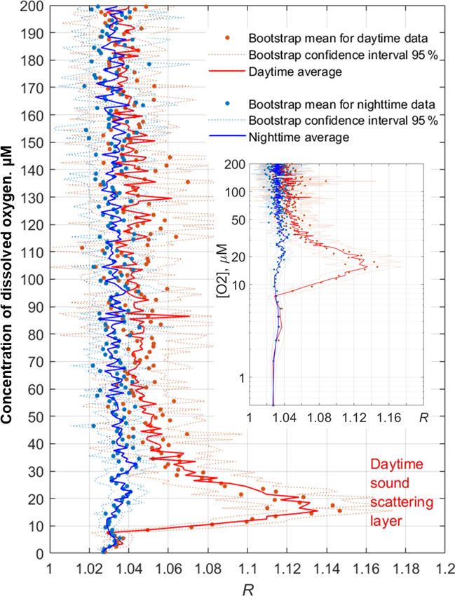
A. G. Ostrovskii et al.: Seasonal variation of the sound-scattering zooplankton vertical distribution                                    959

Figure 3. Diurnal motions of the sound-scattering layers in the oxic
zone. The depth–time scatterplot for profiles of acoustic backscatter
amplitude at 2 MHz was obtained using the Aquadopp instrument at
the moored profiler during verification study involving net sampling
of zooplankton on 21 and 22 June 2010.

noflagellate Noctiluca scintillans, chaetognaths Parasagitta
setosa, and varia (ctenophores Pleurobrachia pileus, appen-
dicularians, meroplankton, decapod larvae, Pisces ova).
   One method for calculating vertical migration speed of
zooplankton from the sound backscatter data of the acous-
tic current meter at the profiler Aqualog was described in
Pezacki et al. (2017). However, the vertical migration speed
of mesozooplankton is beyond the focus of this study. Only
once when discussing the pattern of the diel vertical mi-
gration is the slope of the migration track on the echogram
(see Fig. 9 below) considered to give a rough idea about the
dive and the ascent of mesozooplankton. Much more effort
would certainly be needed to visualize the specimens’ verti-
cal swimming.

3     Results

3.1    Acoustic scattering by mesozooplankton
       aggregations

The first validation data for the Aquadopp observations were
obtained on 21 and 22. June 2010. The sound-scattering lay-             Figure 4. The diel changes in vertical distributions of (left) total
ers were identified at the raw echogram (Fig. 3) as mesozoo-            mesozooplankton biomass, (middle) zooplankton composition, and
plankton aggregations by comparison with the net sampling               (right) temperature (T ) and density (σ2 ) near the mooring site on 21
data (Fig. 4). The zooplankton net sampling data were con-              and 22 June 2010. The temperature and density profiles were used
sistent with the acoustic backscatter, indicating short-term            for the selection of sampling strata. CE – Calanus euxinus; PE –
variations in biomass and diel vertical migration of zooplank-          Pseudocalanus elongatus; SC – small crustaceans; NS – Noctiluca
ton.                                                                    scintillans; PE – Parasagitta setosa; Var – varia.
   The total mesozooplankton biomass in the entire water
column varied from 0.99 to 3.57 g DW m−2 . Zooplankton

https://doi.org/10.5194/os-17-953-2021                                                                   Ocean Sci., 17, 953–974, 2021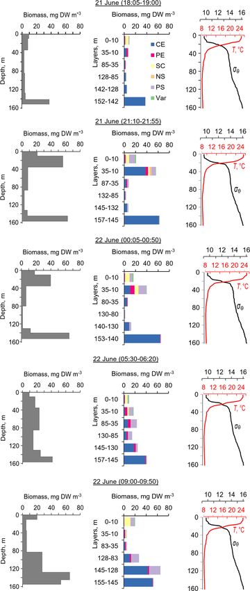
960                  A. G. Ostrovskii et al.: Seasonal variation of the sound-scattering zooplankton vertical distribution

was dominated by the copepod Calanus euxinus, which made        tic scattering by clouds of particles sinking through the water
up the mean 58 % with the standard deviation (SD) ± 14 %        column can obscure zooplankton aggregations.
of the total biomass (below for the sake of brevity, such es-      The layers of elevated acoustic backscatter amplitude due
timates are denoted as mean ± SD%). The contribution of         to deep zooplankton aggregations are accounted for using
chaetognaths Parasagitta setosa was 21 ± 11 %, followed by      the R graphs (Fig. 5b) that were validated by net sampling
copepods Pseudocalanus elongatus (13 ± 7 % of the total         on 6 October 2013 (Fig. 6), although sampling was not per-
biomass). The sum share of other groups of mesozooplank-        formed at night due to stormy weather. Since the depths of
ton did not exceed 7 % of the total biomass.                    the isopycnals of 15.9 and 15.7 differed by only 3 m, the
   The pattern of the vertical distribution of mesozooplank-    integrated zooplankton sample was taken in the layer be-
ton biomass reveals a relatively uniform distribution over      tween σ2 = 15.9 and σ2 = 15.4. In this layer, the contribu-
depth in the evening twilight (18:05–19:00) and at dawn         tions of Calanus euxinus, Parasagitta setosa, and Pseudo-
(05:30–06:20) (Fig. 4, left column). At night (21:10–21:55      calanus elongatus to the total biomass were 60 %, 26 %, and
and 00:05–00:50), the highest concentration of zooplankton      12 %, respectively (Fig. 6b). The extremely low zooplankton
was observed in the thermocline layer, while in the daytime     biomass (< 2 mg DW m−3 ) in the upper 50 m layer (Fig. 6a
(09:00–09:50), the zooplankton maximum was in the layer         and b) is consistent with data on a 4-fold decrease in the an-
between the density surfaces σ2 15.7 and 15.4 (Fig. 4, left     nual average biomass of upper dwelling zooplankton in 2013
column), in accordance with the diurnal changes in the vol-     compared to previous years (Arashkevich et al., 2015).
ume backscatter strength (Fig. 3). The deepest layer bounded       Zooplankton diel vertical migration trajectories in the
by isopycnals σ2 15.9 and 15.7 was inhabited by nonmigrat-      R graph are noticeably clear below 40 m (Fig. 5b). The ex-
ing copepods, the fifth copepodite stage (CV) of C. euxinus     planation of these phenomena could be that the scattering
(median prosome length 2.3 mm), persistently staying at this    area of the elongated bodies of the zooplankton species is
depth throughout the day (Figs. 3 and 4, middle column).        larger in the horizontal projection than in the inclined projec-
Visual inspection of live samples revealed quiescent behav-     tion at an angle of 45◦ . Therefore, the orientation of the bod-
ior of these specimens and large oil sac volume inside their    ies of mesozooplankton species appears to be mainly verti-
body, suggesting a diapausing state in C. euxinus CV col-       cal during migration. At night, these specimens are randomly
lected from the deepest layer (Vinogradov et al., 1992).        oriented in the upper layer, where R ≈ 1. In addition to the
   Three migrating species, copepodites CIV–CVI of C. eu-       diel vertical migrations, intraday vertical fluctuations of zoo-
xinus (median prosome length 2.6 mm), CV–CVI P. elon-           plankton occur with an inertial period (Fig. 5b). The vertical
gatus (median prosome length 0.92 mm), and chaetognaths         displacements of the daytime deep mesozooplankton aggre-
P. setosa (median length 19 mm), formed daytime zooplank-       gations are coherent with the vertical displacements of both
ton aggregations in the oxygen-deficient zone (Fig. 4, mid-     isopycnals and isooxylines. The displacements of isopycnals
dle column). Ctenophore Pleurobrachia pileus, also inhabit-     with amplitudes up to 20 m are mainly due to near-inertial
ing the deep layers in the daytime, contributed negligibly to   waves.
the total biomass due to the low dry matter content in their       In October 2016, persistent aggregation of diapausing
gelatinous bodies and their low abundance (shown as Var in      C. euxinus was detected in the acoustic backscatter signal
Fig. 4). At night, most of the migrating zooplankters were      (Fig. 7), unlike October 2013 (Fig. 5). Zooplankton sampling
concentrated in the thermocline and did not ascend to the       was performed at midnight and midday on 4 and 5 October
warm UML, which was inhabited by small copepods, clado-         2016 (Fig. 8). The pattern of zooplankton distribution was
cerans, and small (< 6 mm) chaetognaths.                        similar to that in June 2010 (Fig. 4), both in terms of the to-
                                                                tal biomass and composition of zooplankton and in terms of
                                                                the day–night vertical distribution. The total mesozooplank-
3.2   Zooplankton aggregations visualized using the
                                                                ton biomass of 1.8–2.3 g DW m−2 was dominated by three
      directional acoustic backscatter ratio
                                                                species: C. euxinus (59 %–76 %), P. setosa (9 %–22 %), and
                                                                P. elongatus (5 %–10 %). At night, the maximum aggregation
The echograms based on the data from horizontal-beam            of migrating zooplankters was in the thermocline layer, and
transducers A1 and A2 often reveal aggregations of zoo-         at midday, it was in the layer between isopycnals σ2 15.7
plankton at depths of 80–120 m in the daytime (Fig. 5). The     and 15.4 (Fig. 8a). Daytime zooplankton aggregation con-
aggregations begin to rise around sunset and descend before     sisted mainly of C. euxinus (92 % of total biomass) with a
dawn. Thin, nearly vertical lines on the echogram indicate      small contribution from chaetognaths (7 % of total biomass)
acoustic traces of the migrating mesozooplankton species.       (Fig. 5b). The layer between isopycnals σ2 15.9 and 15.7
The echogram also shows patches that occupy the entire wa-      was persistently occupied by diapausing C. euxinus CVs. The
ter column, from the upper to the lower measurement depth,      chaetognaths found in this layer were represented by spent
penetrating below the surface σ2 15.9 and then deeper into      specimens and corpses (Fig. 8b). UML was inhabited by non-
the hydrogen sulfide zone. These are clouds of suspended        migrating small copepods, cladocerans, and small chaetog-
particles (see, for example, Klyuvitkin et al., 2016). Acous-   naths.

Ocean Sci., 17, 953–974, 2021                                                       https://doi.org/10.5194/os-17-953-2021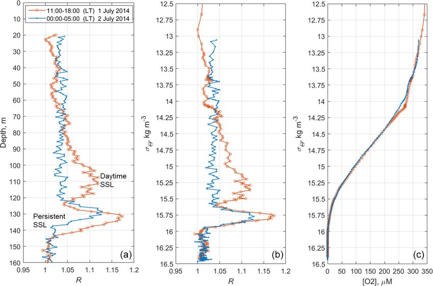
A. G. Ostrovskii et al.: Seasonal variation of the sound-scattering zooplankton vertical distribution                                       961

Figure 5. (a) The time–depth graph of the Aquadopp horizontal-beam (A1 +A2 )/2 echogram showing acoustic backscatter intensity (counts)
on 5–7 October 2013. The Aqualog profiler with the Aquadopp instrument performed ascending–descending cycles every 1 h. The upper,
middle, and lower white lines are for isopycnals σ2 15.4, 15.7, and 15.9, respectively. (b) Time–depth scatterplot of the Aquadopp directional
acoustic backscatter ratio R = (A1 + A2 )/2A3 . Colored lines show [O2 ] = 50 µm (upper black line); [O2 ] = 10 µm (lower black line); and
σ2 = 15.9 kg m−3 (white line), which can be taken as a proxy for the boundary of the oxygen zone in the NE Black Sea (Glazer et al., 2006,
Ostrovskii and Zatsepin, 2016). Notice that due to upwelling, the oxycline was moved upward. Vertical dotted white lines indicate a 17.3 h
time interval, which is equal to the period of inertial oscillations at the latitude of the observation. They approximately coincide with troughs
of inertial waves.

   The net sampling data on the day–night vertical distribu-                  The two-layered structure was also observed at the end
tion of mesozooplankton agreed broadly with the acoustic                   of June–early July 2014 (Fig. 9) and validated by day–night
backscatter observations obtained during the next few days                 zooplankton sampling on 1 and 2 July (Fig. 10). Deeper zoo-
(Fig. 7). On the echogram, one can see a persistently existing             plankton aggregation was monospecific, consisting only of
backscattering layer associated with the isopycnal layer near              diapausing C. euxinus CVs (Fig. 10b) and formed a thin layer
σ2 = 15.9, as well as patches of the high-volume backscatter-              (5–10 m thick). This layer was visible all day and night and
ing strength at depth during the daytime and their movement                was usually located above the isopycnal surface of 15.9. It is
into shallower layers at night.                                            clearly distinguished by the value R > 1.1 (Fig. 9b). The day-
                                                                           time zooplankton aggregation consisted of three migrating

https://doi.org/10.5194/os-17-953-2021                                                                       Ocean Sci., 17, 953–974, 2021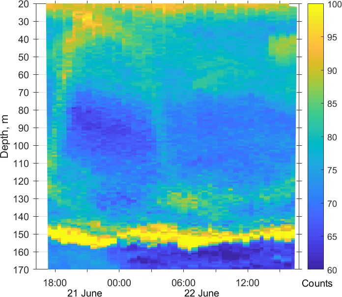
962                   A. G. Ostrovskii et al.: Seasonal variation of the sound-scattering zooplankton vertical distribution

Figure 6. The daytime vertical distributions of (a) total mesozooplankton biomass, (b) zooplankton composition, and (c) temperature (T )
and density (σ2 ) near the mooring site at 12:30–13:20 on 6 October 2013. Temperature and density profiles (c) indicate the selection of
sampling strata. CE – Calanus euxinus; PE – Pseudocalanus elongatus; SC – small crustaceans; NS – Noctiluca scintillans; PE – Parasagitta
setosa; Var – varia.

                                                                       species and their different developmental stages, C. euxinus,
                                                                       CIV–CVIs, P. elongatus, CV–CVIs, and P. setosa, 14–22 mm
                                                                       in size (Fig. 10b). Since the amplitude of vertical migration
                                                                       is different for different components of this assembly, the
                                                                       daytime deep aggregation reached 35 m in thickness. Before
                                                                       sunset, migrating zooplankters began to move upward and at
                                                                       night formed aggregations at depths above 40 m (Fig. 9a) and
                                                                       peaked in the thermocline at 17–25 m (Fig. 10a).
                                                                          Since migrating zooplankton aggregations were observed
                                                                       in the deep layers only during the daytime, it is worth com-
                                                                       paring the daytime average R profile with that for the night-
                                                                       time (Fig. 11). Such a comparison clearly reveals the deep
                                                                       maximum of R at the daytime migration depths of mesozoo-
                                                                       plankton at 90–120 m, as well as the persistent maximum of
                                                                       the diapause layer within the deeper layer at 125–140 m. No-
                                                                       tably, the depths of the persistent SSL change by approxi-
                                                                       mately 5 m from night to the daytime, while they completely
                                                                       overlap when considered vs. the density. Such variations in
                                                                       the depth of the SSL might be linked to inertial oscillations
                                                                       (Ostrovskii et al., 2018).

                                                                       3.3   The seasonal variation in mesozooplankton
                                                                             dynamics in relation to dissolved oxygen
                                                                             concentration

                                                                       In Sect. 3.2, it was shown that the mesozooplankton species
                                                                       float on isopycnals in the lower part of the oxycline and
                                                                       in the hypoxic zone. Both the diapausing aggregations and
                                                                       the daytime aggregations are displaced coherently by near-
                                                                       inertial waves. The deep aggregations of mesozooplankton
                                                                       are bounded by certain isopycnal surfaces and isooxylines.
Figure 7. (a) The time–depth scatterplot of the Aquadopp                  Since the oxygen stratification strongly depends on the
horizontal-beam echo (A1 + A2 )/2 on 6–10 October 2016. (b) The        density stratification in the pycnocline (e.g., Vinogradov and
time–depth graph of the Aquadopp directional acoustic backscatter      Nalbandov, 1990; Codispoti, et al., 1991; Konovalov et al.,
ratio R. The isopycnals and isooxylines are superimposed near the      2005; see also example in Fig. 12), it becomes possible to
SSLs.                                                                  switch from the depth profiles of the directional acoustic
                                                                       backscatter ratio R(z), where z is the depth, to the R([O2 ])

Ocean Sci., 17, 953–974, 2021                                                               https://doi.org/10.5194/os-17-953-2021
A. G. Ostrovskii et al.: Seasonal variation of the sound-scattering zooplankton vertical distribution 963 Figure 8. Day–night vertical distribution of (a) total mesozooplankton biomass, (b) zooplankton composition, and (c) temperature (T , ◦ C) and density (σ2 ) near the mooring site at 22:00–23:00 on 4 October (night) and 11:05–11:50 on 5 October (day) 2016. Temperature and density profiles (c) indicate the selection of sampling strata. CE – Calanus euxinus; PE – Pseudocalanus elongatus; SC – small crustaceans; NS – Noctiluca scintillans; PE – Parasagitta setosa; Var – varia. profiles to investigate the seasonal changes of the sound- layer shifts in the lower part of the suboxic zone where scattering mesozooplankton layers in terms of R vs. [O2 ]. [O2 ] = 3–7 µm. It becomes substantially weaker in Septem- The average monthly profiles of R([O2 ]) were constructed ber. In October, this layer degrades further. In November, it from R(z) and [O2 ](z) data for every month when the data tends to disappear. were available. To compute the averages, the daytime was defined as a period beginning 2 h after the local time of sun- rise (at a given date) and ending 2 h before sunset. The night- 4 Discussion time was defined as a period beginning 1 h after sunset and ending 1 h before sunrise. Example plots of the average pro- 4.1 Visualization of the sound-scattering files hR([O2 ])i computed as arithmetic and bootstrap mean mesozooplankton aggregations values along with 95 % bootstrap confidence intervals are shown for November 2019 in Fig. 13. In the hypoxic zone, Previously, acoustic measurements at a frequency of 2 MHz the average values hR([O2 ])i for the daytime are significantly were not considered a tool for observations of the mesozoo- higher than those for the nighttime. The daytime averages plankton SSLs in the sea due to the limited range of sound- hR([O2 ])i > 1.06 were in the range of [O2 ] = 9–40 µm in ings. However, with the advent of ocean profilers with acous- November 2019. tic Doppler current meters, such as the Nortek Aquadopp, The average monthly hR([O2 ])i profiles show the seasonal it has become possible to obtain the depth profiles of the evolution of the mesozooplankton distribution (Fig. 14). The volume scattering strength at 2 MHz frequency in the en- SSLs are barely discernible in January. One can note some tire water column and to study the vertical distribution of activity in the upper part of the oxycline in February. Al- zooplankton, such as those in the Black Sea (Ostrovskii and though we unfortunately do not have data for March, in Zatsepin, 2011; Pezacki et al., 2017). Acoustic sounding of April, two peaks appear in the hR([O2 ])i profiles in the mesozooplankton at two angles is made possible using the layers where the concentration of dissolved oxygen is 25– side-looking head of the Nortek Aquadopp instrument. The 60 µm and 4–9 µm. These maxima correspond to the day- combination of horizontal and tilted beam signals allows, time mesozooplankton aggregations and the diapause layer, on the one hand, the patches of particles to be eliminated respectively. The upper maximum of hR([O2 ])i, which cor- and the background scattering level of the echogram to be responds to the daytime aggregations of mesozooplankton, equalized and, on the other hand, the preferred orientation of may weaken in June–July. However, it becomes stronger mesozooplankton species migrating through the oxycline to again at the end of summer and in autumn. The largest be determined. Earlier, Stanton and Chu (2000) reproduced value for this maximum over the entire observation period the influence of the orientation of a 3 mm calanoid copepod hR([O2 ])i = 1.18 is observed in October. At that time, the (modeled as a high-resolution approximation of an animal maximum shifts into the layer where [O2 ] is 10–25 µm. In profile) on the acoustic target strength at 2 MHz with re- December 2019, this peak was between the 10 and 30 µm spect to an incident sonar beam. The reduction was found to isooxylines. be 5 %–15 % when copepod orientation was shifted from 0◦ The maximum of diapause mesozooplankton was (broadside incidence) to 30–60◦ . Benfield et al. (2000) car- strongest in May and July 2020, reaching almost 1.2 at ried out field observations using the Video Plankton Recorder [O2 ] = 5–8 µm. In August, the diapause mesozooplankton on George Bank and showed that most Calanus finmarchi- https://doi.org/10.5194/os-17-953-2021 Ocean Sci., 17, 953–974, 2021
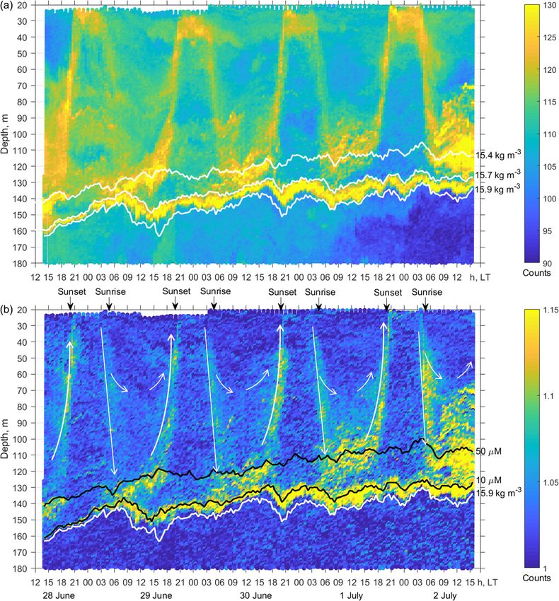
964                    A. G. Ostrovskii et al.: Seasonal variation of the sound-scattering zooplankton vertical distribution

Figure 9. (a) The time–depth graph of the Aquadopp horizontal-beam echo (A1 +A2 )/2 during the moored profiler survey on 28 June–2 July
2014. The isopycnals are superimposed near the SSLs. (b) The graph of time–depth variation in R based on the measurements of sound
backscattering. The upper and lower black lines are isooxylines of 50 and 10 µm, respectively. The white line indicates isopycnal σ2 = 15.9.
There is a persistent SSL under isooxyline [O2 ] = 10 µm. Thin white arrows schematically show the diel migration of mesozooplankton.
The maximum depth of the diel vertical migration is 120–150 m, although some specimens dive to depths of only 80–100 m. The slope
of the straight arrow pointing downwards corresponds to a diving speed of ∼ 1.5 cm s−1 . The ascent is accelerated and reaches values of
approximately 2.5 cm s−1 in the upper 60 m depth.

cus (75 %) in the depth range of 10–70 m were within ± 30◦              how the orientation of individuals changes with depth to
of the prosome-up or prosome-down orientation. It was sug-              correctly account for the biomass of mesozooplankton. Ex-
gested that one reason for the behavior underlying the head-            periments using a multiple-angle acoustic receiver array on
up orientation pattern might be due to the predator avoidance           live copepods and mysids in a laboratory tank showed that
strategy aimed at reducing the conspicuousness of C. fin-               it is possible to use the scattered acoustic signal to distin-
marchicus when viewed from above. Such individuals would                guish among zooplankton taxa (Roberts and Jaffe, 2008). Re-
present a significantly reduced cross-sectional area to an              flections in the frequency range from 1.5 to 2.5 MHz were
echo-sounder’s transducer with correspondingly diminished               recorded from untethered 1–4 mm calanoid copepods and 8–
target strength. It was concluded that it is necessary to know          12 mm mysids over an angular range of 0–47◦ . That study

Ocean Sci., 17, 953–974, 2021                                                                 https://doi.org/10.5194/os-17-953-2021
A. G. Ostrovskii et al.: Seasonal variation of the sound-scattering zooplankton vertical distribution                                  965

Figure 10. The day–night vertical distribution of (a) total mesozooplankton biomass, (b) zooplankton composition, and (c) temperature (T )
and density (σ2 ) near the mooring site on 1 July (13:30–14:30) and 2 July (02:30–03:30) 2014. Temperature and density profiles (c) indicate
the selection of sampling strata. CE – Calanus euxinus; PE – Pseudocalanus elongatus; SC – small crustaceans; NS – Noctiluca scintillans;
PE – Parasagitta setosa; Var – varia.

Figure 11. The time averages of R and [O2 ] for the daytime of 1 July 2014 (red) and the nighttime of 2 July 2014 (blue), when net sampling
(Fig. 10) took place. (a) The depth profiles of the time averages R. (b) The daytime and nighttime averages R vs. the specific density, σ2 .
(c) Distribution of the daytime and nighttime averages of the dissolved oxygen concentration vs. σ2 .

demonstrated the utility of a multiple-angle acoustic array             ter measurements suggested by models (Stanton and Chu,
for zooplankton identification.                                         2000; Roberts and Jaffe, 2007) and laboratory experiments
   To distinguish the SSLs against the background patterns              (Roberts and Jaffe, 2008). Since the late 1990s, researchers’
of vertical flow of settling particles and to study the orien-          efforts have been focused on creating multichannel instru-
tation of zooplankton species, we propose a simple method               ments to measure acoustic backscatter (volume scattering
for the processing of ultrasound sensing data at three angles.          strength) at several frequencies, which contain information
This acoustic three-beam geometry provides a partial prag-              about the size composition of the scatterers, since differ-
matic solution for the quest towards the multiple-angle scat-           ent frequencies bounce off objects of different sizes (Wiebe

https://doi.org/10.5194/os-17-953-2021                                                                   Ocean Sci., 17, 953–974, 2021
966                     A. G. Ostrovskii et al.: Seasonal variation of the sound-scattering zooplankton vertical distribution

Figure 12. (a) Example of the monthly long time series of the
vertical profiles of the directional acoustic backscatter ratio R for
November 2019 (in total 960 profiles from the moored profiler sur-
vey). The upper and lower black lines are isooxylines of 50 and
10 µm, respectively. The white line indicates isopycnal σ2 = 15.9.       Figure 13. Example profiles of the daytime and nighttime averages
(b) Evolution of the dissolved oxygen at the profiler mooring site       hR([O2 ])i in November 2019. The inset shows the same plots with
in November 2019. The colored lines indicate the following: the          the y axis drawn logarithmically to reflect the lower parts of the
depths of the isopycnals σ2 = 14 and 15.9 (top and bottom white          profiles (the hypoxic zone) in more detail.
lines); the depth of the temperature minimum (green line); and
[O2 ] = 50 and 10 µm (blue lines). The inset shows the diagram
of the concentration of dissolved oxygen vs. the potential den-
sity, [O2 ] − σ2 , plotted from the moored profiler data of November
2019. In this example, as well as for other observational periods, the   by sampling narrow depth strata (10–15 m layers) targeting
concentration of dissolved oxygen deviates very little from isopyc-      deep-water aggregations visualized on the echograms. The
nal surfaces in the lower part of the oxycline where [O2 ] < 200 µm.     two-layered structure of the aggregations seen on echograms
                                                                         and R graphs in the daytime (Figs. 3, 7, and 9) reflected the
                                                                         species composition of zooplankton in these layers (Figs. 4,
et al., 2002; Smeti et al., 2015). Multichannel instruments              8, and 10). The deepest layer bounded by isopycnals 15.9 and
in conjunction with video cameras are fairly expensive sys-              15.7 was visible in the suboxic zone all day and night and
tems that are used for the identification of mesozooplank-               was formed by diapausing CV Calanus euxinus. To some ex-
ton in its natural habitat. Plausibly, a multichannel three-             tent, this monospecific layer was contaminated by crustacean
angle system featuring several relatively cheap short-range              exuviae and carcasses, spent females, and zooplankters’ re-
three-beam acoustic units each operating at an individual fre-           mains sinking from the upper layers and apparently retained
quency when installed on a vertically profiling carrier would            on the density gradient. The existence of a nonmigrating dia-
be a very effective tool for visualizing zooplankton aggrega-            pausing stock located in the suboxic layer from mid-spring to
tions.                                                                   mid-autumn is confirmed by observations from submersible
                                                                         Argus (Vinogradov et al., 1985; Flint 1989), by high verti-
4.2   The SSLs validated from the stratified net sampling                cal resolution sampling with 150 L water bottles (Vinogradov
                                                                         et al., 1992), and by zooplankton net sampling (Arashkevich
Comparison of the Nortek Aquadopp acoustic backscatter                   et al., 1998; Besiktepe, 2001; Svetlichny et al., 2009). How-
observations with the data obtained by stratified zooplankton            ever, for some unknown reasons, this nonmigrating layer was
sampling showed good agreement of the features of the diel               not detected by shipborne echo sounders at frequencies of
vertical distribution of zooplankton. This was made possible             38–200 kHz (Erkan and Gücü, 1998; Mutlu, 2003, 2007; Ste-

Ocean Sci., 17, 953–974, 2021                                                                 https://doi.org/10.5194/os-17-953-2021
A. G. Ostrovskii et al.: Seasonal variation of the sound-scattering zooplankton vertical distribution 967 Figure 14. Top – the monthly averaged profiles of hR([O2 ])i for the daytime over the upper part of the continental slope near Gelendzhik in the NE Black Sea. Bottom – the same for the nighttime. https://doi.org/10.5194/os-17-953-2021 Ocean Sci., 17, 953–974, 2021
968                  A. G. Ostrovskii et al.: Seasonal variation of the sound-scattering zooplankton vertical distribution

fanova and Marinova, 2015; Sakınan and Gücü, 2016), unlike        ano, 2020). The mesozooplankton that feed at the surface but
our data obtained by Aquadopp at a frequency of 2 MHz.            metabolize and excrete at depth contribute to the transport of
   The inclusion of diapause (or dormant stage) in the life       organic matter; more quantitatively, this contribution is esti-
cycle of all Calanidae species living in high-latitude and        mated to be between approximately 10 %–50 % of the local
temperate environments is well known (e.g., see review in         sinking flux of organic particles (Bianchi et al., 2013, and
Baumgartner and Tarrant, 2017). Having accumulated a large        references therein).
amount of lipids, diapausing copepods descend into deeper            In the lower part of the oxic zone, the vertical displace-
ocean layers, where they can exist for several months at the      ments of SSLs coincide with the oscillations of isopycnal sur-
expense of energy reserves. Decreased metabolic rate and          faces (Figs. 5 and 10). The dissolved oxygen concentration
developmental delay are characteristic features of diapaus-       profile tightly hinges on the density stratification in the Black
ing copepods. In the Black Sea, a decrease in the metabolic       Sea since both are basically due to vertical mixing processes
rate in diapausing C. euxinus is caused not only by inter-        (e.g., Ostrovskii et al., 2018). Hence, displacements of the
nal physiological reasons, but also by hypoxia in their dor-      SSLs with regard to the oxy-isolines are much smaller than
mant layer. The oxygen consumption rate in diapausing CV          those vs. the depths. The vertical oscillations with a period
C. euxinus in hypoxia decreases by almost an order of mag-        of approximately 17 h near the mooring site are due to near-
nitude, and the rate of ammonia excretion decreases 6 times       inertial waves (Ostrovskii et al., 2018). Irregular changes in
compared with those in their active counterparts in normoxia      isopycnal depths occur due to hydrodynamic events, such as
(Svetlichny et al., 1998).                                        individual internal waves, oceanic fronts, and jets. Occasion-
   During the daytime, the upper SSL mostly located above         ally, the isopycnal depth may change by 30–40 m within a
σ2 = 15.7 consisted of four species, copepods C. euxinus and      day (Ostrovskii and Zastsepin, 2016).
Pseudocalanus elongatus, chaetognaths Parasagitta setosa,            It is unlikely that copepods maintain their positions on
and ctenophores Pleurobrachia pileus; the latter had a negli-     certain isopycnal surfaces by swimming, as displacements
gible contribution to dry biomass. This assembly had a wide       of such large amplitudes by tens of meters require an addi-
range of body lengths from approximately 1 mm in P. elonga-       tional depletion of energy reserves. A more beneficial strat-
tus to 22 mm in P. setosa. The different species had different    egy would be to adjust their buoyancy to neutral. Having
swimming speeds. It was also possible that these species had      neutral buoyancy in the hypoxic zone, the copepods would
different physiological tolerances to oxygen deficiency. This     not need to spend much additional energy floating up and
confirms earlier observations from the manned submersible,        down following crests and troughs of internal waves while
which showed that the daytime aggregation of migrating zoo-       avoiding entrainment into the suboxic layer. Indeed, direct
plankton had a layered structure: the lower layer was formed      observations from manned submersibles revealed a quiescent
by chaetognaths, whereas the older stages of C. euxinus were      behavior of diapausing copepods and their slow response to
located above, and ctenophores inhabited the upper part of        light and noise produced by underwater vehicles, both in the
the aggregation (Vinogradov et al., 1985; Flint, 1989). Fur-      Santa Barbara Basin (Alldredge et al., 1984) and in the Black
thermore, the different developmental stages of copepods          Sea (Mikhail Flint, personal communication, 2020). Neutral
C. euxinus and P. elongatus occupied different depths, deep-      buoyancy has been hypothesized to be regulated by changes
ening as their size increased (Morozov et al., 2019).             in lipid composition (Visser and Jónasdóttir, 1999); however,
   In the evening, approximately 2 h before sunset, zooplank-     Campbell and Dower (2003) argued that this buoyancy reg-
ters begin to ascend to the upper layers, where they spend all    ulation mechanism is inherently unstable because wax esters
the dark hours concentrating in the thermocline layer and be-     are more compressible than seawater. An alternative mech-
low it. In this layer, while feeding, they move in different      anism for buoyancy regulation in diapausing copepods that
directions and are oriented randomly (Kiørboe et al., 2009),      involves the replacement of heavy ions with lighter ammo-
so they cannot be discernible in the R graphs. According to       nium ions in hemolymph has been proposed by Sartoris et al.
our data, cold-water herbivorous C. euxinus and P. elongatus      (2010) by analogy with other invertebrates. Later, Schründer
only occasionally ascend into the warm UML, mainly inhab-         et al. (2013) found high concentrations of ammonium ions
iting colder layers rich in phytoplankton (see also the supple-   in the hemolymph of a diapausing species, Calanoides acu-
ment to the paper by Morozov et al., 2019). Predator chaetog-     tus, and suggested that these copepods could achieve neu-
naths P. setosa move upward following copepods, their main        tral buoyancy through their biochemical body composition
prey (Drits and Utkina, 1988). The time of zooplankton mi-        without swimming movements. This mechanism obviously
gration clearly visible on the echograms is confirmed by the      would better explain the observed phenomenon of diapaus-
results of net sampling and is consistent with other published    ing copepod movement synchronized with the displacements
data (see for reference the Supplement of Morozov et al.,         of the isopycnal surfaces in the Black Sea.
2019).
   The vertical migration of zooplankton can increase the
vertical flow of carbon and thus contribute to the function-
ing of the biological pump in the ocean (Tutasi and Escrib-

Ocean Sci., 17, 953–974, 2021                                                          https://doi.org/10.5194/os-17-953-2021
You can also read