Understanding the relative importance of vertical and horizontal flow in ice-wedge polygons - Hydrol-earth-syst-sci.net
←
→
Page content transcription
If your browser does not render page correctly, please read the page content below
Hydrol. Earth Syst. Sci., 24, 1109–1129, 2020
https://doi.org/10.5194/hess-24-1109-2020
© Author(s) 2020. This work is distributed under
the Creative Commons Attribution 4.0 License.

Understanding the relative importance of vertical and horizontal
flow in ice-wedge polygons
Nathan A. Wales1,2 , Jesus D. Gomez-Velez2,3 , Brent D. Newman1 , Cathy J. Wilson1 , Baptiste Dafflon4 ,
Timothy J. Kneafsey4 , Florian Soom4 , and Stan D. Wullschleger5
1 Los Alamos National Laboratory, Los Alamos, NM, 87545, USA
2 Hydrology  Program, Department of Earth & Environmental Science, New Mexico Institute of Mining
and Technology, Socorro, NM, 87801, USA
3 Department of Civil and Environmental Engineering, Vanderbilt University, Nashville, TN, 37235, USA
4 Earth Science Division, Lawrence Berkeley National Laboratory, Berkeley, CA, 94720, USA
5 Environmental Sciences Division, Oak Ridge National Laboratory, Oak Ridge, TN, 37831-6301, USA

Correspondence: Nathan A. Wales (nathanwales@gmail.com)

Received: 15 January 2019 – Discussion started: 1 April 2019
Revised: 18 December 2019 – Accepted: 27 January 2020 – Published: 10 March 2020

Abstract. Ice-wedge polygons are common Arctic land-               these systems. This work forms a basis for understanding
forms. The future of these landforms in a warming climate          complexity of flow in polygonal landscapes.
depends on the bidirectional feedback between the rate of
ice-wedge degradation and changes in hydrological charac-
teristics. This work aims to better understand the relative
roles of vertical and horizontal water fluxes in the subsurface    Copyright statement. The United States Government retains, and
of polygonal landscapes, providing new insights and data to        the publisher, by accepting this work for publication, acknowledges
                                                                   that the United States Government retains, a nonexclusive, paid-up,
test and calibrate hydrological models. Field-scale investi-
                                                                   irrevocable, worldwide license to publish or reproduce this work or
gations were conducted at an intensively instrumented loca-        allow others to do so for United States Government purposes.
tion on the Barrow Environmental Observatory (BEO) near
Utqiaġvik, AK, USA. Using a conservative tracer, we ex-
amined controls of microtopography and the frost table on
subsurface flow and transport within a low-centered and a          1   Introduction
high-centered polygon. Bromide tracer was applied at both
polygons in July 2015 and transport was monitored through          A mechanistic understanding of the feedbacks between Arc-
two thaw seasons. Sampler arrays placed in polygon centers,        tic climate and terrestrial ecosystems is critical to under-
rims, and troughs were used to monitor tracer concentra-           stand and predict future changes in these sensitive ecosys-
tions. In both polygons, the tracer first infiltrated vertically   tems. Observations suggest that high-latitude systems are ex-
until encountering the frost table and was then transported        periencing the most rapid rates of warming on Earth, lead-
horizontally. Horizontal flow occurred in more locations and       ing to increased permafrost temperatures, melting of ground
at higher velocities in the low-centered polygon than in the       ice, and accelerated permafrost degradation (Hinzman et al.,
high-centered polygon. Preferential flow, influenced by frost      2013; Jorgenson et al., 2010; Romanovsky et al., 2010). Per-
table topography, was significant between polygon centers          mafrost degradation is of primary concern in the Arctic, as
and troughs. Estimates of horizontal hydraulic conductivity        it affects hydrology (Jorgenson et al., 2010; Liljedahl et al.,
were within the range of previous estimates of vertical con-       2011; Zona et al., 2011a), biogeochemical transformations
ductivity, highlighting the importance of horizontal flow in       (Heikoop et al., 2015; Lara et al., 2015; Newman et al.,
                                                                   2015), and human infrastructure (Andersland et al., 2003;
                                                                   Hinzman et al., 2013). The northernmost Arctic permafrost

Published by Copernicus Publications on behalf of the European Geosciences Union.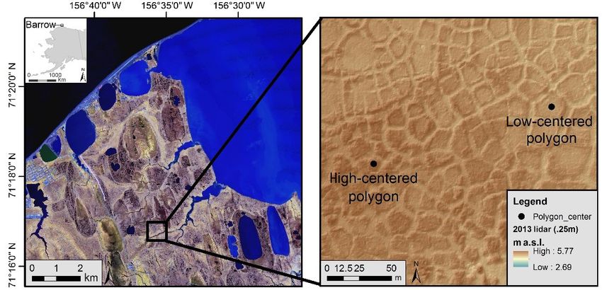
1110                                                        N. A. Wales et al.: Understanding the relative importance of flow

zone covers 24 % of the landmass in the Northern Hemi-             and horizontal subsurface water fluxes in these landscapes,
sphere and stores an estimated 1.7 billion tons of organic         providing insight and data to revise, test, and calibrate per-
carbon (Hugelius et al., 2013; Schuur et al., 2008, 2015;          mafrost hydrology representations in these models.
Tarnocai et al., 2009; Zimov et al., 2006), with a significant        To this end, a tracer study was conducted on polygonal
fraction stored in the Arctic tundra, where ice-wedge poly-        ground in the Barrow Peninsula of Alaska from July 2015
gons are among the most prolific geomorphological features         to September 2016. The Barrow Peninsula is located on the
(Hussey and Michelson, 1966). The degree of soil saturation        Arctic Coastal Plain adjacent to the Arctic Ocean. Approx-
influences whether carbon is released as carbon dioxide or         imately 65 % of the land cover in the Barrow Peninsula is
methane, thus highlighting the importance of understanding         ice-wedge polygonal ground, making this an ideal place to
the hydrology of permafrost regions.                               study the hydrology of ice-wedge polygons (Bockheim and
   Ice-wedge polygons form as thermal contraction creates          Hinkel, 2010). To the best of our knowledge, and with the
cracks in the ground. Each year, with spring snowmelt, these       exception of an invasive and localized dye tracer experiment
cracks collect water, which subsequently freezes to form an        (Boike et al., 2008), this is the first non-invasive tracer study
ice wedge below the surface (Liljedahl et al., 2016). Over         to be conducted at the polygon scale. Furthermore, this ex-
time, the ice wedge grows, displacing ground and eventually        periment is unique in that a tracer was continually monitored
forming a low-centered polygon (Fig. 1). When ice wedges           simultaneously on both a low- and high-centered polygon
around a low-centered polygon degrade, the ground above            throughout thaw seasons, making it possible to characterize
them subsides, inverting the topography and creating a high-       the breakthrough curves and determine times of first arrivals.
centered polygon (Gamon et al., 2012; Jorgenson and Os-            Therefore, our approach permits a comparison of behaviors
terkamp, 2005). These two polygon types represent the ge-          in low- and high-centered polygons over the same time pe-
omorphological end members of ice-wedge polygons. All              riod and meteorological conditions.
polygons have three primary microtopographic features: cen-           The purpose of this paper is to examine how differently
ters, rims, and troughs. A low-centered polygon is defined as      low- and high-centered polygons behave hydrologically and
an ice-wedge polygon with the topographic low at the cen-          to evaluate the relative importance of vertical and horizon-
ter and is characterized by low, saturated centers and troughs     tal flux within polygon systems (including the controls of the
with high and relatively dry rims. A high-centered polygon is      frost table and microtopography on subsurface hydrology).
defined as an ice-wedge polygon with the topographic high          The presence of significant horizontal flow can guide new
at the center and is characterized by low, saturated troughs       upscaling approaches to incorporate these landscape features
and high, dryer centers and rims.                                  into regional hydrologic and biogeochemical models, which
   It is now established that significant hydrological and bio-    traditionally conceptualize the subsurface flow within ice-
geochemical differences exist on the sub-meter scale and are       wedge polygons as exclusively vertical (Chadburn et al.,
influenced by ice-wedge polygon type and microtopographic          2015b; Clark et al., 2015). Insights from this study are in-
features (Andresen et al., 2016; Lara et al., 2015; Liljedahl et   tended to inform future work on the possible effects of per-
al., 2016; Newman et al., 2015; Wainwright et al., 2015). Per-     mafrost degradation by improving the conceptualization used
mafrost degradation has the potential not only to change mi-       in the Arctic Terrestrial Simulator, developed by the Depart-
crotopographic features of ice-wedge polygons, but their hy-       ment of Energy at Los Alamos National Laboratory (Atchley
drologic regimes as well. Understanding hydrologic regimes         et al., 2015; Painter et al., 2016) The Arctic Terrestrial Sim-
can help determine the fate of organic matter and nutrients        ulator performs calculations at the polygon scale and scales
in these landforms. For example, whether organic matter is         up to a watershed scale. Our primary focus is the hydrology
decomposed into carbon dioxide or methane is largely deter-        of the active layer, which is the portion of the soil profile that
mined by local hydrology.                                          thaws each year (Hinzman et al., 1991), with some emphasis
   Many studies have focused specifically on ice-wedge poly-       on surface water. Possible mechanisms of flow heterogeneity
gons, (e.g., Boike et al., 2008; Heikoop et al., 2015; Jor-        are also discussed.
genson et al., 2010; Lara et al., 2015; Newman et al., 2015)
and provided much needed conceptualization (Helbig et al.,
2013; Liljedahl et al., 2016). However, to our knowledge, few      2     Materials and methods
studies have been focused on quantifying the difference in
relative roles of subsurface horizontal fluxes between low-        2.1    Site description
and high-centered polygons, or characterizing heterogeneity
of subsurface flow and transport within these landforms. Fur-      The study site is located east of Utqiaġvik (formerly Barrow),
thermore, most regional and pan-Arctic land models ignore          AK, USA, on the Arctic Coastal Plain in the Barrow Envi-
horizontal flux and focus only on the representation of verti-     ronmental Observatory (Fig. 2). The climate of this region
cal water fluxes in the form of infiltration and evapotranspi-     is characterized by long winters and short summers, with a
ration (Chadburn et al., 2015a, b; Clark et al., 2015). There      mean average annual temperature of −10.2 ◦ C, and mean an-
exists a need to better quantify the relative roles of vertical    nual precipitation of 141.5 mm (NOAA-NCDC, 2000–2016).

Hydrol. Earth Syst. Sci., 24, 1109–1129, 2020                                    www.hydrol-earth-syst-sci.net/24/1109/2020/
N. A. Wales et al.: Understanding the relative importance of flow                                                                 1111

Table 1. Response and recovery data from observation wells. Bold font indicates wells in polygon centers. Change in head 1h (m), time to
peak Tpeak (d), and characteristic response λ (d). N/A = not available; the data necessary to make this estimate was not available.

                                                       LCP                                                 HCP
                                 LWC       LW1      LW2      LW3     LW4     LW5      HWC     HW1     HW2      HW3      HW4     HW5
  2015    event 1    1h (m)       N/A      N/A       N/A      N/A     N/A     N/A      N/A     N/A     N/A       0.06    0.06    N/A
                     Tpeak (d)    N/A      N/A       N/A      N/A     N/A     N/A      N/A     N/A     N/A       0.22    0.28    N/A
                     λ (d)        357     1352      2425      909    1315    1552      N/A     714     714       116     213     417
          event 2    1h (m)      0.166    0.018    0.013     0.576   0.024   0.013     N/A    0.018    0.06      0.15   0.183   0.098
                     Tpeak (d)    0.75     0.73     0.35      0.32    0.75    0.35     N/A     0.32    0.78      0.40    0.79    0.80
                     λ (d)          57      143     N/A         68      85      91     N/A      101      76        72      78     101
          event 3    1h (m)       0.09     0.03     0.03      0.02    0.04    0.03     0.18    0.08     0.07     0.14    0.13    0.08
                     Tpeak (d)    1.96     1.88     1.75      0.89    1.90    1.75     1.05    1.93     2.93     1.00    2.00    1.97
                     λ (d)         333   84 854   19 846       667    N/A     N/A        70    714     1313      204     400     556
          event 4    1h (m)       0.03     0.03     0.02      N/A     0.02    0.02     0.13    0.03    0.03      0.08    0.04    0.03
                     Tpeak (d)    1.32     1.30     1.30      N/A     1.30    1.30     1.42    1.28    1.29      1.40    1.32    1.30
                     λ (d)        N/A      N/A      N/A       N/A     N/A     N/A        66    588     500       286     909     714
          event 5    1h (m)       N/A      N/A      0.01      0.02    N/A     N/A      0.08    N/A     0.02      0.05    0.02    N/A
                     Tpeak (d)    N/A      N/A      0.64      0.66    N/A     N/A      1.72    N/A     0.46      2.11    2.65    N/A
                     λ (d)        286      N/A      N/A       909    1043     N/A        87    909     500       233     244     N/A
          event 6    1h (m)       0.05     0.03     0.01      0.01    0.02    0.01     0.17    0.03     0.03     0.11    0.10    0.04
                     Tpeak (d)    1.75     2.95     0.96      1.34    1.00    0.95     1.13    1.02     1.05     1.23    2.70    1.42
                     λ (d)        N/A      N/A      N/A       N/A     N/A     N/A        66    714     2345      204     N/A     N/A
          event 7    1h (m)       0.05     0.04      0.03     0.02    0.03    0.03     0.22    0.04    0.03      0.06    0.05    0.03
                     Tpeak (d)    1.28     1.19      1.38     1.25    1.20    1.38     0.38    0.34    0.33      0.46    1.36    0.35
                     λ (d)       1532      556      1219      556     588    1000        70    357     385       244     417     556
          event 8    1h (m)       0.03     0.02      0.03     0.02    0.02    0.03     0.17    0.03    0.02      0.04    0.02    0.03
                     Tpeak (d)    0.86     1.17      1.18     1.07    0.84    1.18     0.85    0.75    0.81      0.89    1.08    0.78
                     λ (d)         769     714      1687     1827     667     909        57    455     526       333     455     476
  2016    event 9    1h (m)       N/A      0.01      N/A      0.01    N/A     N/A      0.02    0.02    0.02      0.03    0.05    N/A
                     Tpeak (d)    N/A      0.42      N/A      0.34    N/A     N/A      0.31    0.39    0.34      0.34    0.74    N/A
                     λ (d)         29      833       625     1528    2851    1324       455    435     417       714     130     N/A
          event 10   1h (m)       0.13     0.01      0.03     N/A     0.02    0.01     N/A     0.03    0.01      N/A     0.11    N/A
                     Tpeak (d)    0.79     0.84      0.85     N/A     0.83    1.08     N/A     0.20    0.20      N/A     0.77    N/A
                     λ (d)         115     625      1134     2220     833     667      N/A     345     556       N/A     114     N/A
          event 11   1h (m)       0.10     0.01     0.02      0.03    0.01    0.01     N/A     0.01    N/A       N/A     0.12    N/A
                     Tpeak (d)    0.41     1.24     1.23      0.36    1.12    1.27     N/A     0.26    N/A       N/A     0.44    N/A
                     λ (d)         250     556      455       244     556    1000      N/A     152     286       N/A     118     N/A
          event 12   1h (m)       N/A      N/A       N/A      N/A     N/A     N/A      N/A     N/A     N/A       N/A     N/A     N/A
                     Tpeak (d)    N/A      N/A       N/A      N/A     N/A     N/A      N/A     N/A     N/A       N/A     N/A     N/A
                     λ (d)        303      N/A       556      385     769     909      N/A     333     417       N/A     N/A     270
          event 13   1h (m)       0.29     0.08      0.11     0.16    0.09    0.08     0.12    0.16    0.20      0.26    0.31    0.27
                     Tpeak (d)    5.89     6.53      6.50     5.43    6.54    6.56     5.49    6.49    6.50      5.49    6.49    5.47
                     λ (d)         238    1432      1553      400    1320    2106        53    556     556       156     313     435
          event 14   1h (m)       0.18     0.09      0.04     0.07    0.09    0.08     0.23    0.09     0.09     0.17    0.15    0.12
                     Tpeak (d)    4.07     5.14      2.96     3.00    5.06    7.17     1.75    1.85     2.98     3.00    4.16    3.34
                     λ (d)         714    1720      3125     1323    1857    6025        52    769     1000      333     625     769

www.hydrol-earth-syst-sci.net/24/1109/2020/                                          Hydrol. Earth Syst. Sci., 24, 1109–1129, 2020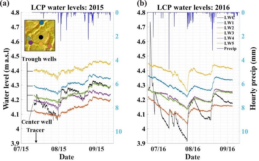
1112 N. A. Wales et al.: Understanding the relative importance of flow
Figure 1. Conceptual diagram of a low-centered polygon (a) and a high-centered polygon (b). Porosity and Ksat (m s−1 ) values from the
literature (see Supplement, Table S1: Atchley et al., 2015; Beringer et al., 2001; Hinzman et al., 1991; Lawrence and Slater, 2008; Letts et
al., 2000; Nicolsky et al., 2009; O’Donnell et al., 2009; Price et al., 2008; Quinton et al., 2000; Zhang et al., 2010).
The coldest temperatures occur in February with warmest tures (Kanevskiy et al., 2013). Patterns of cryogenic struc-
temperatures in July (NOAA-NCDC, 2000–2016). The thaw tures found in frozen soils can result in higher porosities than
season usually begins in June with maximum thaw depth oc- found in unfrozen soils (Dafflon et al., 2016).
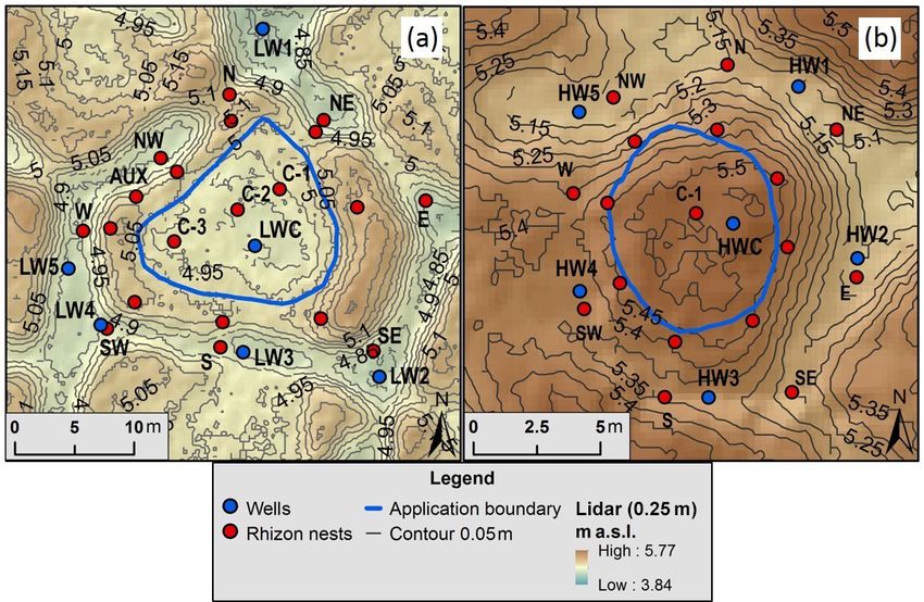
curring sometime in late August or early September. Freeze- One high-centered polygon (with an area of 132 m2 ) and
up typically begins sometime in September, subsequently one low-centered polygon (with an area of 706 m2 ) were cho-
leaving the ground completely frozen until June when the sen to reflect the extremes of tundra polygon morphology
next thaw season begins. After the brief snowmelt period, a (Fig. 3). Only two polygons were used to minimize anthro-
receding water table despite precipitation indicates that evap- pogenic perturbations to the study site and because the cost
otranspiration dominates during the first half of the thaw sea- and logistical complexity of these experiments is significant.
son while a rising water table with precipitation indicates that Even though this limits our ability to replicate the results,
precipitation and infiltration dominate during the second half the polygons selected are representative of a larger inven-
of the thaw season. These observations are consistent with tory of low- and high-centered polygons being investigated
observations of evapotranspiration during the 2 years prior by our team at this intensive study site and have similar size
to the tracer experiment described here (Raz-Yaseef et al., and morphology, providing new insight into hydrologic dif-
2017) and in other previous studies on Arctic water balances ferences between polygon types and into flow and transport
(Helbig et al., 2013; Pohl et al., 2009). across polygon features. The general soil profile of the poly-
The region is characterized by low-relief land forms un- gons was an organic layer, comprised of 2–20 cm moss and
derlain by continuous, perennially frozen permafrost > 400 m peat (Iversen et al., 2015), underlain by a seasonally thawed
thick and an active layer depth ranging from 30 to 90 cm mineral soil layer, followed by permafrost (Fig. 1). Ice lenses
(Hinkel et al., 2003; Hubbard et al., 2013). The soil profile can form during freeze-up, especially in the mineral soil.
consists of an organic layer typically < 40 cm thick under-
lain by a silty mineral layer composed primarily of quartz 2.2 Observational network
and chert (Black, 1964; Hinkel et al., 2003). The volume of
shallow ground ice in the region can be as high as 80 % and
Each polygon had been instrumented with six fully screened
is comprised primarily of ice wedges and cryogenic struc-
observation wells (3.81 cm diameter PVC casing), one in the
Hydrol. Earth Syst. Sci., 24, 1109–1129, 2020 www.hydrol-earth-syst-sci.net/24/1109/2020/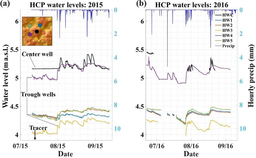
N. A. Wales et al.: Understanding the relative importance of flow                                                                     1113

Figure 2. Map showing the portion of the Barrow Peninsula where the study was conducted (left) and a close-up of the area containing the
low- and high-centered polygons used for the tracer study.

Figure 3. Digital elevation model for the low-centered (a) and high-centered (b) polygons. Red dots represent locations of sampler nests
and blue dots represent locations of observation wells. Blue circle indicates area of tracer application and encompasses the polygon center:
167.4 m2 for the low-centered polygon and 41.6 m2 for the high-centered polygon. Note scales are different for the two polygons.

center of the polygon and five distributed along the surround-             To prevent preferential flow along the well casings,
ing troughs (blue circles in Fig. 3). All well casings were             15.24 cm diameter PVC pipe was placed around each well
surveyed using a dGPS unit. Pressure transducers (Diver,                casing and pressed through the organic layer into the
Schlumberger Water Services, Netherlands) were deployed                 top 2 cm of the mineral layer (Fig. 4a). Silicon sheets
in each well to measure stage fluctuations at 15 min intervals          30.5 cm × 30.5 cm × 0.24 cm with pre-cut holes were also
and used to estimate water table elevations relative to ground          placed around each 15.24 cm pipe at the ground level to form
surface (measured in meters above sea level, m a.s.l.). Baro-           a watertight seal. Additional silicon sheets of the same di-
metric data were also collected at the study site and used to           mensions were placed around the samplers (discussed below)
correct water level data for barometric effects. The pressure           to prevent preferential or wall flow along the outer casing of
transducers have an accuracy of ±0.5 cm of H2 O and a reso-             the samplers. Caps were also placed on samplers between
lution of 0.2 cm of H2 O.                                               sampling events to prevent precipitation from collecting in-

www.hydrol-earth-syst-sci.net/24/1109/2020/                                           Hydrol. Earth Syst. Sci., 24, 1109–1129, 2020
1114                                                            N. A. Wales et al.: Understanding the relative importance of flow

                                                                       (Fig. 4b). An additional sampler nest was placed in the rim
                                                                       of the low-centered polygon where a saddle occurred, con-
                                                                       stituting an area of interest due to possible flow convergence.
                                                                       To minimize perturbations and avoid the generation of pref-
                                                                       erential flow paths, samplers at frost table depth were not re-
                                                                       moved prior to freeze-up at the end of the 2015 thaw season.
                                                                       As a result, in 2016, the deepest samplers were not sampled
                                                                       until the frost table reached the deepest depth for 2015.

                                                                       2.3   Bromide tracer test

                                                                       Bromide was used as a tracer due to its conservative nature
                                                                       with low potential for adsorption and ion exchange and neg-
Figure 4. (a) Schematic representation of the observation wells with   ligible background concentrations (Davis et al., 1980). Other
isolation sleeve and (b) a schematic representation of a Rhizon sam-   tracers were considered, but low background levels of bro-
pling nest.
                                                                       mide had been previously established (Newman et al., 2015),
                                                                       and given the high organic matter content and low pH of ac-
                                                                       tive layer waters, bromide was thought to be the best option.
side the housing of the samplers and diluting samples. Pre-            Potassium bromide (KBr) was dissolved in water and ap-
cipitation was measured using a tipping gauge rain bucket,             plied to the interior of each polygon with a garden sprayer
65 m from the study site.                                              (167.4 m2 for the low-centered polygon and 41.6 m2 in the
   MacroRhizon samplers (Rhizosphere Research Products,                high-centered polygon: outlined in blue in Fig. 3). A refer-
Netherlands) were used to sample pore water at various loca-           ence grid of nylon cord was used to guide the even distribu-
tions and depths in both study sites (Fig. 4b). These samplers         tion of tracer, and disposable rubber booties and latex gloves
minimize perturbations to the porous media matrix and flow             were worn during application to prevent contamination out-
field by collecting sample volumes at low rates, no greater            side of the application area. A total of 8 L of tracer solu-
than 60 mL d−1 , driven by the suction of a syringe at the sur-        tion with a concentration of 5000 mg L−1 (40 g of Br) was
face. In addition, the sampler dimensions made it feasible             applied to the high-centered polygon on 12 July 2015 and
to simultaneously sample three soil depths within a 12 cm              24 L of tracer solution with a concentration of 10 000 mg L−1
diameter circle. Each sampler collected water through a tip            (240 g of Br) was applied to the low-centered polygon on
9 cm in length and 4.5 mm diameter with a mean pore size               13 July 2015. The higher concentration and volume used in
of 0.45 µm. In this work, sample depths refer to the inser-            the low-centered polygon compensated for the surface area,
tion depth of sampler tip ends (Fig. 4b). In most cases, sy-           about 3 times larger than the high-centered polygon. A total
ringes remained on the samplers overnight to collect suf-              of 10 L of water was subsequently sprayed on each polygon
ficient sample volumes, and therefore some sampling peri-              to facilitate infiltration of tracer into the soil.
ods spanned over 24 h. When freezing temperatures were ex-
pected overnight, sampling was initiated and collected on the          2.4   Sampling and analytical methods
same day.
   The rims of each polygon had eight nests of MacroRhi-               Sampling frequency in the MacroRhizon samplers varied
zon samplers oriented in a radial pattern around the poly-             depending on precipitation events and observed tracer con-
gon (Fig. 3). Each sampler nest had samplers at three depths:          centrations. In 2015, samples were typically taken every 2
15 cm, 25 cm, and at the frost table. Samplers at the 15 and           and 4 d during periods with and without precipitation events,
25 cm depths were fixed over time while the deepest sampler,           respectively. We sampled daily during periods of persis-
installed once the frost table reached a depth of 35 cm, was           tent daily precipitation events. A full suite of samples was
moved downward on a weekly basis as the frost table depth              taken prior to tracer application to establish background
increased. Troughs surrounding each polygon also had eight             levels of bromide. Pre-deployment bromide concentrations
nests of samplers adjacent to corresponding sampler nests on           were consistent with those previously observed in the area
the rims (Fig. 3). Three nests of samplers were placed in the          (Newman et al., 2015), and many pre-deployment concen-
center of the low-centered polygon and only one in the cen-            trations were at or near the limit of detection of the ion
ter of the high-centered polygon due to its smaller relative           chromatograph used for analysis (0.01 ppm). In addition to
area. Unlike the sampling nests in rims and troughs, sam-              groundwater samples, grab samples of surface waters were
plers in polygon centers were inserted at 45◦ so the sampling          also collected during each sampling event. Samples were
tips would protrude past the edges of the silicon sheets. Sam-         frozen and shipped to the Geochemistry and Geomaterials
plers in polygon centers were inserted to depths of 15 cm and          Research Laboratory (GGRL) at Los Alamos National Lab-
25 cm, and frost table depth was sampled at 35 cm and deeper           oratory (LANL) for analysis. Samples were thawed and fil-

Hydrol. Earth Syst. Sci., 24, 1109–1129, 2020                                       www.hydrol-earth-syst-sci.net/24/1109/2020/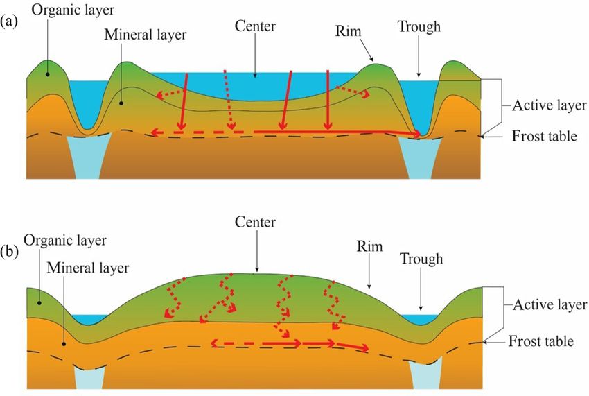
N. A. Wales et al.: Understanding the relative importance of flow 1115
tered through a 0.45 µm syringe filter prior to analysis via ion were kept frozen and, a few days after drilling, transported
chromatography with an uncertainty of ±5 %. frozen to Lawrence Berkeley National Laboratory (LBNL) in
Frost table depth measurements, taken with a tile probe, Berkeley, CA. Three-dimensional images of the cores were
were typically taken weekly to the nearest 0.5 cm at each obtained using a medical X-ray computed tomography (CT)
sampler nest. This served the dual purpose of ensuring the scanner at 120 kV. Images were reconstructed to resolutions
deepest sampler was at the depth of the frost table and mea- of 2.56 pixels per millimeter or better in the core-horizontal
suring frost table depth. In both polygons, the frost table gen- plane and 0.625 mm along the core-vertical axis. Additional
erally reached its deepest point in the beginning of Septem- cores containing ice lenses were extracted from the frozen
ber. Within the low-centered polygon, the maximum frost ta- active layer using a 51 mm diameter AMS soil auger. Cores
ble depth measured over the two thaw seasons was 43 cm in were kept frozen until subsampling at the Permafrost Labo-
the center, 45 cm in the rims, and 50 cm in the troughs. The ratory at the University of Alaska Fairbanks.
maximum measured frost table depths for the high-centered
polygon were 45 cm in the center, 43.5 cm in the rims, and 2.7 Well response and recovery
38 cm in the troughs for both field seasons.
To better understand the response of the polygons to precip-
2.5 Ground-penetrating radar itation inputs, we focused on the temporal characteristics of
water level changes caused by 14 precipitation events occur-
Ground-penetrating radar (GPR) surveys were conducted on ring over the 2015 and 2016 thaw seasons (Fig. 5). Each of
each polygon to understand the influence of frost table to- these events is preceded and followed by relatively dry pe-
pography on flow (Dafflon et al., 2015). GPR has been used riods, resulting in water level changes with clear ascending
for various applications in Arctic regions including estima- and recovery curves. Isolating the water level hydrograph as-
tion of thaw layer thickness (Bradford et al., 2005; Hub- sociated with each precipitation event allowed us to estimate
bard et al., 2013), characterization of permafrost and ice- the maximum change in head (1h), time-to-peak (Tpeak ), and
wedge structure (Léger et al., 2017; Munroe et al., 2007), characteristic recession time (λ) (Table 1). The characteristic
and mapping of snow thickness (Wainwright et al., 2017). In recession time is calculated as the reciprocal of the slope for
this study, common-offset surface GPR transects were col- the line fitted to the natural log of water table elevation ver-
lected on 2 October 2015 to estimate thaw layer thickness sus time during the recession limb. This recession time is a
at the low- and high-centered polygon locations. GPR data simple measure of the memory of the well to perturbations
were collected using a Mala Ramac system with 500 MHz caused by precipitation events (Troch et al., 2013).
antennas along four ∼ 34 m long parallel transects crossing 2.8 Tracer arrival and hydraulic conductivity
the low-centered polygon, and along 51 ∼ 15 m long SE-
NW transects spaced 0.25 m apart crossing the high-centered The temporal evolution of tracer concentrations at selected
polygon. A wheel odometer was used to acquire traces with observation wells was used to approximate average linear ve-
a spacing of 0.06 m. Minimal processing of the common off- locities and bulk hydraulic conductivity values for each poly-
set lines included zero-time adjustment, bandpass filtering, gon. To this end, velocities were estimated by assuming that
automatic gain control, semi-automated picking of the two- the transport of the tracer within the polygons can be approx-
way travel time to the key reflector, and conversion of travel imated as a one-dimensional advective–dispersive problem
time to depth. The key reflector corresponds to the interface with adsorption effects – a reasonable assumption given the
between the thaw layer and the permafrost, as confirmed by lack of information and uncertainty in the spatial distribution
the strong relationship between the GPR signal travel time of hydraulic parameters. This is a parsimonious approach to
and manual probe-based measurements of thaw layer thick- explore the first-order factors controlling fate and transport
ness (correlation coefficient ∼ 0.73). The relationship has and timescales within this complex system. Van Genuchten
been used to convert the GPR signal travel time to thaw layer and Alves (1982) found an analytical solution to this problem
thickness. Frost table elevation was obtained by subtracting for the case of a semi-infinite soil profile without production
the GPR-inferred thaw layer thickness from the digital eleva- or decay and with a constant initial concentration:
tion model of the study site. Given the high spatial density of
GPR data at the high-centered polygon location, a frost table Ci + (C0 − Ci ) A (x, t) 0 < t < t0
elevation map was obtained through linear interpolation. c (x, t) = Ci + (C0 − Ci ) A (x, t) t > t0 (1)
−C0 A (x, t − t0 ) ,
2.6 Core analyses with
Rx − vt
Shallow cores were extracted, using a SIPRE auger, from A (x, t) = 0.5 erfc
areas adjacent to the polygon tracer studies. Each core was 2(DRt)0.5
collected from the frozen active layer at a different location. Rx + vt
Cores were 46 mm in diameter and the lengths varied. Cores + 0.5 experfc (2)
2(DRt)0.5
www.hydrol-earth-syst-sci.net/24/1109/2020/ Hydrol. Earth Syst. Sci., 24, 1109–1129, 2020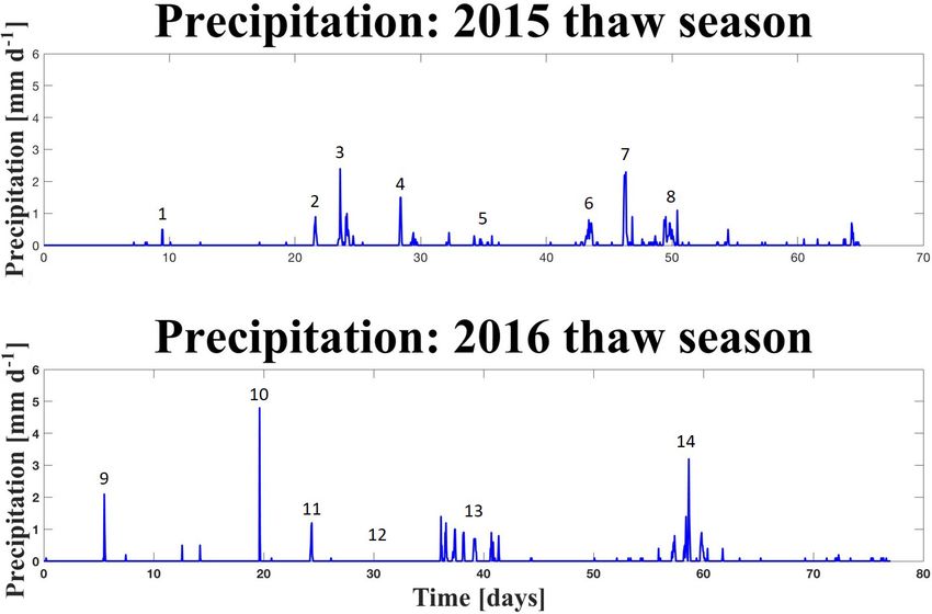
1116                                                           N. A. Wales et al.: Understanding the relative importance of flow

Figure 5. Precipitation events, from 3 July 2015 to 30 September 2016, used in the calculation of characteristics of well response. Note that
event 12 is not a precipitation event, but marks where a recession limb was analyzed for each well.

and initial and boundary conditions given by                             breakthrough above background level (Ci ). These times and
                                                                         the parameters specified above were used to approximate lin-
c (x, 0) = Ci ,
                                                                        ear velocities and bulk hydraulic conductivity values for each
             C0    0 < t < t0 ,                                          polygon.
c (0, t) =
             0     t > t0 ,                                                 Consistent with the experiment, the arrival time for a sam-
dc                                                                       pler located at a distance x = L is significantly larger than
    (∞, t) = 0.                                                          the duration of tracer application, ta  to , warranting the ap-
dt
                                                                         proximation ta −t0 ≈ ta and reducing Eq. (1) to the following:
In Eqs. (1) and (2), Ci (mg L−1 ) is initial concentration, Co
(mg L−1 ) is input concentration, t (h) is time, to (h) is dura-         C (x = L, t = ta ) ≈ Ci − Ci A(x = Lt = ta ).                   (3)
tion of solute pulse, and x (cm) is the lateral distance from the
sampling nests to the edge of the tracer application area. The           Substituting Eq. (2) and rearranging, we obtain the follow-
function A(x, t) is the effluent concentration, where R is the           ing:
retardation coefficient (–), v is pore-water velocity (cm h−1 ),
and D (cm2 h−1 ) is the dispersion coefficient.                                  RL − vta              vL         RL + vta
                                                                         erfc                 +  exp      erfc
   We use the conditions in the field experiment to parame-                     2(DRta )0.5            D         2(DRta )0.5
terize Eqs. (1) and (2). Background concentrations and tracer
                                                                                Ci − C (L, ta )

application varied for each polygon (see Table 2). In the                 −2                      = 0.                            (4)
                                                                                     Ci
high-centered polygon, the background concentration was
Ci = 0.19 mg L−1 , and a solution with concentration Co =                   Then, the velocity v is estimated as the root of Eq. (4)
5000 mg L−1 was injected over a period of to = 4.5 h. On                 (see Table 2) and assumes full saturation. Note that other ap-
the other hand, the low-centered polygon had a background                proaches based on the center of mass of the breakthrough
concentration of Ci = 0.44 mg L−1 and a solution with Co =               curve have been previously proposed (Feyen et al., 2003;
10 000 mg L−1 was injected over a period of to = 1.75 h.                 Harvey and Gorelick, 1995; Mercado, 1967); however, they
The dispersion coefficient was constrained to the range 1–               cannot be used in our experiment because only a small frac-
100 cm2 d−1 based on the information available in Fig. 1 and             tion of the tracer was recovered after 2 years of monitoring
Eq. (3) from Gelhar et al. (1992). With an average pH of                 and the complete flushing of the tracer is likely to take sev-
5.6 in the study area (Newman et al., 2015), the retardation             eral more.
factor was approximated as R = 1.56 (Korom, 2000) – a rea-                  Bulk hydraulic conductivities were then estimated using
sonable value given the pH in Korom’s experiment was be-                 the fitted velocity values (Table 2). Vertical velocities were
tween 5.1 and 5.7. Finally, arrival time (t = ta ) for each sam-         estimated by substituting L for the depth of the sampler.
pler was determined by linear interpolation between the first            Horizontal velocities were estimated by substituting L for

Hydrol. Earth Syst. Sci., 24, 1109–1129, 2020                                           www.hydrol-earth-syst-sci.net/24/1109/2020/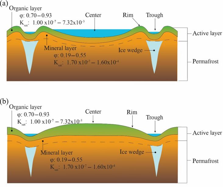
N. A. Wales et al.: Understanding the relative importance of flow                                                                           1117

Table 2. Tracer breakthrough locations, times, and linear velocities. Italic text indicates uncertainty in tracer arrival time due to insufficient
data for interpolation. The ∗ symbol denotes samplers at frost table depth. Bold font denotes vertical flow (center wells) and normal font
denotes horizontal flow.

                                  Low-centered polygon
                                  Location         Distance     Arrival time     Min velocity    Max velocity
                                                       (cm)               (d)       (cm d−1 )       (cm d−1 )
                                  C-1*                  36.5           8±1              2.70             20.97
                                  C-2                     15          24 ± 1            1.55              7.39
                                  C-2∗                    61          23 ± 1            1.60             11.23
                                  C-3∗                    58           6±1              7.40             30.30
                                  S-rim∗                222           23 ± 1            8.53             19.49
                                  NE-rim∗               197           26 ± 1            6.53             16.56
                                  NW-trough∗            363           11 ± 1           17.14             31.33
                                  SE-trough              694          13 ± 1           38.52             51.85
                                  High-centered polygon
                                  Location         Distance     Arrival time     Min velocity    Max velocity
                                                       (cm)               (d)       (cm d−1 )       (cm d−1 )
                                  C-1                    15           21 ± 1             1.64             7.10
                                  C-1                    25           34 ± 1             0.03             5.49
                                  C-1*                   25           21 ± 1             0.22             8.30
                                  SE-rim*               43.5          23 ± 1             0.93             9.20

the shortest horizontal distance from the samplers in rims                 2.9    Mass balance
or troughs to the area of tracer application in the polygon
interior. When estimating horizontal velocities, vertical ar-              While it was not possible to close the mass balance of the
rival times could not be separated from the horizontal arrival             tracer without compromising the experiment (i.e., by coring
times. Thus, resultant estimates for horizontal hydraulic con-             or digging pits) an attempt was made to bracket the mass
ductivity were low bounding estimates.                                     balance. For each polygon, the largest and smallest break-
   Darcy’s law was used to constrain hydraulic conductivity:               through curves via horizontal flux were used to estimate the
                                                                           limits at which horizontal flux had redistributed tracer from
       v h θ Lh                                                            polygon centers to rims and troughs. Only one breakthrough
Kh =            ,                                                 (5)
         1h                                                                curve was used for the high-centered polygon since break-
                                                                           through was only detected at one location outside the poly-
where Kh is the horizontal estimate of hydraulic conductiv-
                                                                           gon center. First, each polygon was idealized as a cylinder
ity, v h is the horizontal estimate of pore velocity, θ is effec-
                                                                           and its area calculated so flux could be estimated. The radius
tive porosity, Lh is horizontal distance, and 1h is the hy-
                                                                           used for the idealized cylinder of the low-centered polygon
draulic head change. Ranges of Kh for each polygon were
                                                                           was 13.4 m and the radius used for the high-centered poly-
estimated using maximum and minimum estimated horizon-
                                                                           gon was 3.8 m. Second, flux was calculated through the side
tal velocities and the minimum and maximum values of min-
                                                                           of the cylinder as the product of the area, porosity, and ve-
eral layer porosity reported in the literature, 0.19 and 0.55,
                                                                           locity. Mineral layer porosity values of 0.19 and 0.55 were
respectively (Beringer et al., 2001; Hinzman et al., 1998;
                                                                           used, representing the minimum and maximum porosity val-
Lawrence and Slater, 2008; Letts et al., 2000; Nicolsky et
                                                                           ues listed above, and the values used for velocity were the
al., 2009; O’Donnell et al., 2009; Price et al., 2008; Quin-
                                                                           previously mentioned linear velocity values. Lastly, the prod-
ton et al., 2000; Zhang et al., 2010). The change in hydraulic
                                                                           uct of the flux and change in tracer concentration over time
head was estimated by finding the average head difference,
                                                                           were integrated with respect to time.
over the course of observation in 2015, between the well in
the polygon center to the well nearest the sampler of interest.

www.hydrol-earth-syst-sci.net/24/1109/2020/                                               Hydrol. Earth Syst. Sci., 24, 1109–1129, 2020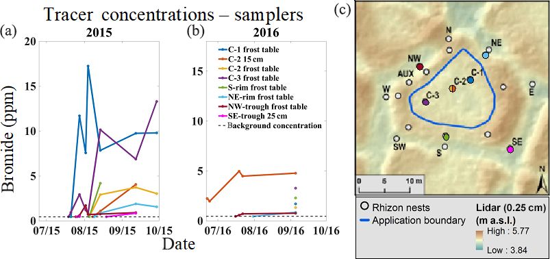
1118                                                        N. A. Wales et al.: Understanding the relative importance of flow

3     Results                                                         At the high-centered polygon, water levels between cen-
                                                                   ter and trough locations often varied by nearly a meter. The
3.1    Flow characteristics (observations)                         center well, HWC, was often dry in the 2016 thaw season
                                                                   as were trough wells HW1, HW2, HW3, and HW5 (Fig. 7).
From the beginning of July until mid-August in each thaw           When the center well was not dry, the water level was typ-
season (2015 and 2016), there was relatively little precip-        ically higher than that of the trough wells, indicating a hy-
itation in the study area and the water table was receding         draulic gradient from the polygon center to the troughs when
(Figs. 6 and 7). In both thaw seasons, most of the precipita-      water was present. Inspection of the well hydrographs reveals
tion occurred between mid-July and the end of August, con-         that the well in the polygon center, HWC, had steeper post-
current with a rising water table. This behavior is explained      precipitation recession limbs than wells in the troughs.
by evapotranspiration dominance during the first half of each         The high-centered polygon most often had higher 1h val-
season, previously observed by Raz-Yaseef et al. (2017), and       ues in the polygon center than in the troughs. Additionally,
infiltration dominance in the second half. Daily average tem-      recession times, λ, were usually shortest in the polygon cen-
peratures fluctuated between −0.7 and 7.8 ◦ C and −1.7 and         ter with longer times in the troughs. As in the low-centered
13.7 ◦ C in the 2015 and 2016 thaw seasons, respectively           polygon, this is consistent with groundwater mounding in the
(NOAA-CRN 2015-2016). We observed that the study site              center with subsequent subsurface horizontal redistribution
was much drier in the 2016 thaw season, with far less stand-       to the troughs. Of the trough wells, HW3 and HW4 tended
ing water in the study area than in the 2015 thaw season.          to have the highest 1h values with shorter recession times,
In addition, overland flow was never observed as a result of       λ, than other trough wells (Fig. 7 and Table 1). Notice that
precipitation events, suggesting high infiltration capacity and    these wells are located in high sections relative to the rest of
dominance of subsurface flow.                                      the trough, but low relative to the polygon center. Further, the
   Water levels in the low-centered polygon varied less than       GPR survey of the high-centered polygon shows that, unlike
40 cm throughout both thaw seasons, with the exception of a        surface topography, most of the frost table in the polygon
peak in the center well in 2016 (Fig. 6) which is most likely      center (the area within the tracer application zone outlined
from meltwater filling the well when the frost table was only      by the blue circle) slopes to the south-southwest (Fig. 8b).
a few centimeters deep. For much of the 2015 thaw season,          This indicates that the majority of mounded groundwater
the water level in the center well was as high as or higher than   from the polygon center is likely redistributed to the south-
three out of five of the trough wells, indicating variable hy-     southwest trough of the polygon at HW3 and HW4. Subse-
draulic gradients across the polygon. Conversely, for most of      quently, mounded water at HW3 and HW4 is redistributed to
the 2016 thaw season, the water level in the center well was       other parts of the polygon trough. Conversely, HW1, HW2,
lower than the wells in the troughs, indicating the possibility    and HW5 usually have smaller 1h, shorter times-to-peak,
of the reversal in the direction of the hydraulic gradient from    and longer recession times indicating that ponding is domi-
the polygon center to troughs. Inspection of the well hydro-       nant in these areas (Table 1).
graphs reveals that the center well responded as quickly as
trough wells to precipitation events, but with faster increases    3.2   Transport characteristics (observations)
in water table elevation and steeper recession limbs.
   In the low-centered polygon, most precipitation events re-      Tracer breakthrough for both polygons did not exhibit
sulted in higher 1h values in the polygon center than in           smooth breakthrough curves typically seen in laboratory
trough wells while characteristic recession times, λ, in the       tracer experiments. Instead, these breakthrough curves have
polygon center were generally shorter than those of trough         a more jagged form, showing sudden changes in concentra-
wells (Table 1). This is consistent with infiltration and pond-    tion. This jagged nature is due partly to sampling frequency.
ing in the center of the polygon with subsequent subsur-           Often, there were several days between sampling events, re-
face horizontal redistribution of mounded groundwater to the       sulting in breakthrough curves with a low temporal resolu-
troughs. When the system is low in storage (i.e., events 2–4)      tion. However, there is also evidence that large rain events
(Fig. 5 and Table 1), Tpeak values tend to be lower in trough      were responsible for some of this variability over time. For
wells than in the center well. Wells located in the troughs are    example, in the low-centered polygon, there was a concentra-
in topographic lows acting as convergence areas where pond-        tion increase in well C-1 at the frost table after precipitation
ing is likely to occur (Fig. 3). Conversely, when the system is    Event 3 (Figs. 5 and 9).
higher in storage (i.e., events 7 and 8), ponding occurs more         At the low-centered polygon, tracer arrived first at the cen-
quickly in the polygon center, resulting in Tpeak values in the    ter samplers, second in the trough samplers, and third at the
polygon center that are shorter or more similar to those in        rim samplers (Fig. 9 and Table 2). Tracer breakthrough in
the troughs. This behavior highlights the importance of mi-        the center had higher concentrations than in rims or troughs.
crotopography and storage on flow within the low-centered          This was expected as the center was the area of tracer ap-
polygon.                                                           plication. While the succession of vertical breakthrough was
                                                                   not entirely captured at all three depths for all three center

Hydrol. Earth Syst. Sci., 24, 1109–1129, 2020                                    www.hydrol-earth-syst-sci.net/24/1109/2020/
N. A. Wales et al.: Understanding the relative importance of flow 1119
Figure 6. Water levels from the low-centered polygon (LCP) for the 2015 (a) and 2016 (b) thaw seasons. Arrow indicates date of tracer
application. Dots in the inset (upper-left) correspond to observation-well locations; colors of the dots correspond to well hydrographs. Dark
blue lines along the top of the graphs indicate hourly total precipitation.
Figure 7. Water levels from the high-centered polygon for the 2015 (a) and 2016 (b) thaw seasons. Dots in the inset (upper-left) correspond
to observation-well locations; colors of the dots correspond to well hydrographs. Dark blue lines along the top of the graphs indicate hourly
total precipitation.
sampling locations in the low-centered polygon, tracer ar- 15 cm depth of the C-2 sampler to 30.3 cm d−1 at the frost
rival times were different for each sampling location in the line of the C-3 sampler (Table 2).
center. Specifically, tracer arrived first at the frost table of the The tracer reached the northeast and southern rim loca-
C-3 sampler after 6 d, then at the frost table of the C-1 sam- tions and the northwest and southeast trough locations of
pler after 8 d, at the frost table of the C-2 sampler after 23 d, the low-centered polygon (i.e., sampling outside the poly-
and finally at the 15 cm depth of the C-2 sampler after 24 d gon center) via subsurface flow paths (Fig. 9). As previously
(Fig. 9 and Table 2). Linear velocities of vertical infiltration, mentioned, no overland flow was observed from polygon
calculated using the Eq. (4), varied from 1.55 cm d−1 at the center to troughs. Interestingly, when tracer breakthrough
was detected at trough locations, there was no breakthrough
www.hydrol-earth-syst-sci.net/24/1109/2020/ Hydrol. Earth Syst. Sci., 24, 1109–1129, 20201120 N. A. Wales et al.: Understanding the relative importance of flow Figure 8. Frost table elevation obtained with a ground-penetrating radar survey at the (a) the low-centered and (b) high-centered polygon locations. Note that transect lines indicate frost table elevation at the low-centered polygon (a) while topographic lines indicate frost table elevation at the high-centered polygon (b). Red arrow indicates the direction of frost table slope in high-centered polygon. Widths of transects on low-centered polygon exaggerated for legibility. See Supplement, Tables S2 and S3 for frost table depths. Figure 9. Tracer breakthrough curves for the low-centered polygon (a) and dots representing their corresponding locations (c). The color of the dots correspond to the breakthrough curve of the same color. The blue line on the polygon digital elevation model (c) depicts the area of tracer application. detected at their adjacent rim locations. In addition, all tracer arrived first at the two trough locations after 11 and 13 d breakthroughs in the rims and the troughs were detected at then at the two rim locations after 23 and 26 d. At the frost table depth except for the southeast trough location, northwest and southeast trough locations, estimated horizon- which occurred at the 25 cm depth. This highlights the in- tal linear velocities ranged from 17.1 to 31.3 and 38.5 to fluence of the frost table topography. 51.8 cm d−1 , respectively. At the northeast and southern rim Tracer was detected at the more distal trough locations locations, estimated horizontal linear velocities ranged from of the low-centered polygon before it was detected at the 6.53-16.5 cm d−1 and 8.53–19.5 cm d−1 , respectively (Fig. 9 relatively proximal rim locations. More specifically, tracer and Table 2). Using Eq. (5), the range of horizontal hydraulic Hydrol. Earth Syst. Sci., 24, 1109–1129, 2020 www.hydrol-earth-syst-sci.net/24/1109/2020/
N. A. Wales et al.: Understanding the relative importance of flow                                                                 1121

                                                                       these concentrations indicate a very small breakthrough, if
                                                                       any.
                                                                          While horizontal hydraulic conductivity estimates were
                                                                       higher for the low-centered polygon than for the high-
                                                                       centered polygon, there was only one estimate for the high-
                                                                       centered polygon. Unlike the low-centered polygon where
                                                                       tracer was applied to a relatively saturated surface, tracer was
                                                                       applied to a dry surface in the high-centered polygon. In both
                                                                       polygons, estimates of horizontal hydraulic conductivity are
                                                                       minimum estimates because vertical arrival times could not
                                                                       be separated from horizontal arrival times.

                                                                       3.3    Mass balance

                                                                       For the low-centered polygon, the largest tracer mass that
Figure 10. Breakthrough curves sampled from the surface waters in      could have left the polygon center was estimated to be
polygon troughs for (a) low-centered polygon in 2015 and (b) low-
                                                                       93.68 % of the tracer. This number is unrealistically high
centered polygon in 2016. Notice the upward trend in tracer con-
                                                                       given that the breakthrough curve used in the estimate was
centration in the troughs of the low-centered polygon (a) during the
2015 thaw season.                                                      incomplete and that the high bounding value used for min-
                                                                       eral porosity was likely overestimated. The smallest tracer
                                                                       mass estimated to have left the center, based on the small-
conductivity based on first arrivals was estimated to be be-           est breakthrough curve, was 4.80 %. This number can be
tween 7.67 × 10⁻⁶ and 9.72 × 10⁻⁴ m s−1 .                              considered a “maximum–minimum” and is likely an over-
   Tracer was also detected in surface water sampled from the          estimate since tracer was not detected at all sampling lo-
troughs around the low-centered polygon. Samples collected             cations around the polygon. For the high-centered polygon,
during 2015 show an increasing trend in tracer concentration           the largest tracer mass that could have left the polygon cen-
near the end of the season (Fig. 10b). Even though surface             ter was estimated to be 6.82 % while the smallest estimated
water tracer concentrations for 2015 were relatively low, sev-         mass was 2.36 %. Again, this number can be considered
eral of the concentrations were above the 0.44 mg L−1 back-            a “maximum–minimum” since the tracer was not detected
ground level for bromide. This observation can be interpreted          at all sampling locations around the polygon. Even though
as an integrated, well-mixed response of all the tracer that           these estimates have large uncertainties, it appears that most
was transported from the polygon center to the troughs via             of the tracer remains within the interior of both polygon cen-
the subsurface. Surface water samples collected from troughs           ters.
during 2016 did not show a clear trend of increasing tracer
concentration (Fig. 10a).                                              4     Discussion
   At the high-centered polygon, tracer arrived first in the
center (C-1) via vertical infiltration, and second in one rim          The general pattern in tracer dynamics in both polygon types
location via subsurface horizontal flux (Fig. 11 and Table 2).         was to first infiltrate vertically until it encountered the frost
The center location exhibited tracer arrival times that did not        table, then to be transported horizontally, highlighting the
necessarily correlate with depth. That is, tracer first arrived        influence of the frost table on horizontal flux. There were
simultaneously at the 15 cm and frost table samplers after             no new tracer arrival locations during the 2016 thaw sea-
21 d, and second at the 25 cm sampler after 34 d. Linear ve-           son beyond those identified in 2015. Only a small percent-
locities of vertical infiltration, calculated from arrival times,      age of tracer mass was recovered after monitoring break-
varied from 0.03 to 8.3 cm d−1 .                                       through over 2 years, indicating that subsurface flow and
   Horizontal tracer flux was evident in only one location             transport within both polygon types was very slow. Ranges
outside the center of the high-centered polygon: the south-            of hydraulic conductivity estimated for both polygons fall
east rim location (Fig. 11 and Table 2). Tracer arrived at the         within the range of vertical conductivity found in the liter-
frost table depth of this location after 23 d. Linear velocity,        ature (Atchley et al., 2015; Beringer et al., 2001; Hinzman
estimated using Eq. (4), was between 0.93 and 9.2 cm d−1 .             et al., 1991, 1998; Lawrence and Slater, 2008; Nicolsky et
The range of horizontal hydraulic conductivity for the high-           al., 2009; O’Donnell et al., 2009; Price et al., 2008; Quin-
centered polygon was estimated to be between 1.27 × 10⁻⁷               ton et al., 2000; Zhang et al., 2010). However, assuming uni-
and 3.65 × 10⁻⁶ m s−1 . Overall, bromide concentrations in             form values for horizontal conductivity is probably inappro-
trough surface waters of the high-centered polygon were low.           priate as there were several rim and trough locations where
While there were only slight concentration increases (around           no tracer was detected.
0.1 mg L−1 ) in three trough locations at the end of 2015,

www.hydrol-earth-syst-sci.net/24/1109/2020/                                         Hydrol. Earth Syst. Sci., 24, 1109–1129, 2020
1122 N. A. Wales et al.: Understanding the relative importance of flow
Figure 11. Tracer breakthrough curves for the high-centered polygon (a) and dots representing their corresponding locations (c). The color
of the dots correspond to the breakthrough curve of the same color. The blue line on the polygon digital elevation model (c) depicts the area
of tracer application.
Overall, the low-centered polygon had higher fluxes and tions (Fig. 9, Table 2). It seems that tracer was able to move
tracer breakthroughs at more locations than in the high- to the trough through areas in between the rim sampler loca-
centered polygon. The observed differences in tracer flux be- tions, at least in the early part of the experiment. For exam-
tween polygon types is, in part, explained by degree of sat- ple, in the low-centered polygon, tracer arrived at the north-
uration. The high-centered polygon, by its very nature, had east trough location, but without ever arriving at the northeast
a higher center relative to the water table and was drier than rim location. This implies that flow paths exist that routed
the center of the low-centered polygon. As a result, the tracer the tracer flux around the adjacent rim location to the corre-
was applied to a more saturated surface on the low-centered sponding trough location. In the high-centered polygon, the
polygon as opposed to a dry surface on the high-centered only breakthrough detected outside the polygon center was at
polygon. This allowed the tracer to become mobile more the southeast rim location (Fig. 11), indicating heterogeneity
quickly in the low-centered polygon even though the eleva- in horizontal transport.
tion gradient was higher in the high-centered polygon. Characteristics of active layer soils help to explain het-
erogeneity of flux. For example, variability in vertical and
4.1 Heterogeneity of flux and contributing factors horizontal flux is consistent with the soil structures observed
in CT scans of cores taken from other ice-wedge polygons
Both polygon tests demonstrate heterogeneity of vertical and near the study area (Fig. 12a and b). Patterns of vertical and
horizontal tracer flux. Preferential flow paths or heterogene- horizontal density contrasts throughout the cores reflect het-
ity of subsurface media likely contribute to the heterogeneity erogeneity and dual porosity of the peat and mineral layers,
of tracer transport observed in both polygon types. Evidence indicating the potential for preferential flow. These patterns
from cores, GPR data, and previous studies provides insight may also be indicative of partial melting or partial freezing
into factors that may be contributing to the heterogeneity of of the soil profile as a driver of heterogeneous flow. Cryotur-
the flow system. The relative importance of these factors still bation, a freeze–thaw process that mixes organic and mineral
needs to be established. soils within the active layer (Bockheim et al., 1998; Michael-
Results suggest heterogeneity in porous media character- son et al., 1996), is also a potential cause of heterogeneity
istics affects vertical transport. Different arrival times at the in subsurface media. Cryoturbation results in discontinuous,
frost table were observed in the low-centered polygon and non-stratified soil horizons. Contrasts in hydraulic properties
various linear velocities were observed in the center of the between discontinuously distributed soil types likely con-
high-centered polygon (Figs. 9, 11 and Table 2). These dif- tributes to heterogeneity in flow and transport.
ferences indicate preferential flow in the vertical direction The influence of frost table topography on horizontal flux
and the existence of secondary porosity. is significant within both polygons. Outside of polygon cen-
The wide range in horizontal hydraulic conductivity ob- ters, tracer was detected almost exclusively at the frost table.
served in both polygons is also characteristic of preferential The structure of frost table topography can be seen through
flow paths or heterogeneous subsurface media. Within the the GPR survey. The GPR transects at the low-centered poly-
low-centered polygon, tracer arrival in the two trough loca- gon show the trend that frost table topography generally fol-
tions was not preceded by tracer arrival in adjacent rim loca-
Hydrol. Earth Syst. Sci., 24, 1109–1129, 2020 www.hydrol-earth-syst-sci.net/24/1109/2020/N. A. Wales et al.: Understanding the relative importance of flow 1123
centered polygons. A frozen core, shown in Fig. 12c, was
collected from saturated tundra at the Barrow Environmental
Observatory. Although this core was not taken from the poly-
gons used in this experiment, it can be used as an analog for
understanding the effect of ice lenses in subsurface structure.
In fully saturated tundra, such as the low-centered polygon,
ice lenses tend to form during freeze-up whereas they are
not as common where tundra is unsaturated, as in the high-
centered polygon. This core, taken from a saturated area, ex-
hibits ice lenses up to 3 mm wide primarily in the horizontal
plane. These structures are consistent with those found in the
transient layer as described by Shur et al. (2005). We specu-
late that, as the active layer progressively thickens each year
and these ice lenses thaw, some of the resultant cracks re-
main open enough to create secondary porosity within the
low-centered polygon. A system of secondary porosity, ori-
ented primarily in the horizontal plane, helps explain why
the low-centered polygon would exhibit faster tracer break-
through in more rim and trough locations and at higher rates
than the high-centered polygon. Whether or not these cracks
stay open, and for how long, may be a function of soil struc-
ture. For example, cracks running through soil containing
high concentrations of decomposed organic matter may col-
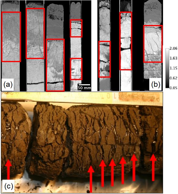
Figure 12. Vertical cross sections of X-ray CT scans of the top lapse more quickly following thaw of ice lenses while cracks
40 cm of cores from (a) low-centered polygons and (b) high- running through soil without decomposed organic matter re-
centered polygons. The CT scans show the density distribution from main longer. Variable collapse of secondary porosity struc-
low (dark) to high (white) with a calibration bar shown in grams per tures across the polygon may help to explain heterogeneity
cubic centimeter (g cm−3 ). Red boxes indicate patterns of vertical of horizontal tracer breakthrough in rims and troughs. Fur-
and horizontal density contrasts. Frozen core sampled from satu-
thermore, thicker and more numerous ice lenses tend to form
rated tundra (c) is analogous to a low-centered polygon. Red arrows
indicate prominent ice lenses. Ice lenses are formed at freeze-up
at the bottom of the active layer, near the top of the per-
when the soil is sufficiently saturated. Notice that most ice lenses mafrost (Guodong, 1983; Shur et al., 2005), helping to ex-
are horizontal relative to ground surface. Photo credit: Vladimir Ro- plain why most breakthrough was observed at the frost table.
manovsky. Additional research is needed to evaluate the importance of
ice lenses on flow and transport within polygon systems.
lows surface topography (Fig. 8). More specifically, higher- 4.2 Transition between 2015 freeze-up and 2016 thaw
elevation frost table areas are overlain by higher-elevation
surface topography and lower-elevation frost table areas are It might be assumed that, due to freezing, tracer migration
overlain by lower-elevation surface topography. Three of the would resume in 2016 where it ended in 2015. However,
four locations where tracer was detected outside the center of in 2016, results show a substantial reduction in tracer con-
the low-centered polygon are where the surface topography, centration as compared to the end of the 2015 thaw season
and therefore the frost table topography, is relatively low in (Figs. 9–11). In fact, concentrations dropped by as much as
the rim separating the polygon center and trough (Figs. 8 and 81 % and many locations with tracer breakthrough in 2015
9). Low points in the topography of the frost table help to ex- did not experience tracer breakthrough until late in the 2016
plain why breakthrough was detected in these locations. This thaw season. Since tracer was mostly detected at frost table
observation is consistent with observations of low-centered depth in 2015, it would have been contained in the frozen
polygons by Helbig et al. (2013) and studies of other Arc- subsurface at the start of the 2016 thaw season. This implies
tic landforms underlain by permafrost (Morison et al., 2017; that tracer would not become mobile in the second year un-
Wright et al., 2009). Similarly, in the high-centered poly- til the active layer thawed to the depth at which the tracer
gon, frost table topography within the application area slopes was frozen in the first year. Even when the ground thawed
to the south-southwest and the only tracer breakthrough de- to depth of the tracer, the tracer could have been further di-
tected outside the polygon center was in the southern half of luted. That is, once the part of the soil profile containing
the polygon (Figs. 8 and 11). tracer begins to thaw it could have also mixed with precip-
The presence of ice lenses may also drive differences itation that had newly entered the system even before all the
in subsurface horizontal flux between the low- and high- tracer-containing ground was thawed. Mixing with precipita-
www.hydrol-earth-syst-sci.net/24/1109/2020/ Hydrol. Earth Syst. Sci., 24, 1109–1129, 2020You can also read