Rapid retreat of permafrost coastline observed with aerial drone photogrammetry
←
→
Page content transcription
If your browser does not render page correctly, please read the page content below
The Cryosphere, 13, 1513–1528, 2019
https://doi.org/10.5194/tc-13-1513-2019
© Author(s) 2019. This work is distributed under
the Creative Commons Attribution 4.0 License.

Rapid retreat of permafrost coastline observed with
aerial drone photogrammetry
Andrew M. Cunliffe1,2 , George Tanski3,4 , Boris Radosavljevic5 , William F. Palmer6 , Torsten Sachs5 , Hugues Lantuit4 ,
Jeffrey T. Kerby7 , and Isla H. Myers-Smith2
1 Geography,  University of Exeter, Exeter, EX4 4RJ, UK
2 School of GeoSciences, University of Edinburgh, Edinburgh, UK
3 Faculty of Sciences, Earth and Climate, Vrije Universiteit Amsterdam, Amsterdam, the Netherlands
4 Department of Permafrost Research, Alfred Wegener Institute, Helmholtz Centre for Polar and

Marine Research, Potsdam, Germany
5 GFZ German Research Centre for Geosciences, Potsdam, Germany
6 Landscapes, Paris, France
7 Neukom Institute for Computational Science, Dartmouth College, Hanover, NH, USA

Correspondence: Andrew M. Cunliffe (a.cunliffe@exeter.ac.uk)

Received: 25 October 2018 – Discussion started: 12 December 2018
Revised: 2 March 2019 – Accepted: 25 April 2019 – Published: 27 May 2019

Abstract. Permafrost landscapes are changing around the           of 2.2 ± 0.1 m a−1 (1952–2017). Coastline retreat rates ex-
Arctic in response to climate warming, with coastal erosion       ceeded 1.0 ± 0.1 m d−1 over a single 4 d period. Over 40 d,
being one of the most prominent and hazardous features.           we estimated removal of ca. 0.96 m3 m−1 d−1 . These find-
Using drone platforms, satellite images, and historic aerial      ings highlight the episodic nature of shoreline change and
photographs, we observed the rapid retreat of a permafrost        the important role of storm events, which are poorly un-
coastline on Qikiqtaruk – Herschel Island, Yukon Territory,       derstood along permafrost coastlines. We found drone sur-
in the Canadian Beaufort Sea. This coastline is adjacent to a     veys combined with image-based modelling yield fine spa-
gravel spit accommodating several culturally significant sites    tial resolution and accurately geolocated observations that
and is the logistical base for the Qikiqtaruk – Herschel Is-      are highly suitable to observe intra-seasonal erosion dynam-
land Territorial Park operations. In this study we sought to      ics in rapidly changing Arctic landscapes.
(i) assess short-term coastal erosion dynamics over fine tem-
poral resolution, (ii) evaluate short-term shoreline change in
the context of long-term observations, and (iii) demonstrate
the potential of low-cost lightweight unmanned aerial ve-         1   Introduction
hicles (“drones”) to inform coastline studies and manage-
ment decisions. We resurveyed a 500 m permafrost coastal          The Arctic is the most rapidly warming region on Earth
reach at high temporal frequency (seven surveys over 40 d in      (Richter-Menge et al., 2017; Serreze and Barry, 2011). In-
2017). Intra-seasonal shoreline changes were related to me-       creasing temperatures result in fundamental changes to the
teorological and oceanographic variables to understand con-       physical and biological processes that shape these permafrost
trols on intra-seasonal erosion patterns. To put our short-term   landscapes (IPCC, 2013). Permafrost in the Northern Hemi-
observations into historical context, we combined our anal-       sphere is substantially degrading in many high-latitude loca-
ysis of shoreline positions in 2016 and 2017 with histori-        tions, resulting in direct and indirect impacts on natural sys-
cal observations from 1952, 1970, 2000, and 2011. In just         tems as well as human activities and infrastructure (Schuur
the summer of 2017, we observed coastal retreat of 14.5 m,        et al., 2015; UNEP, 2012). Coastal erosion is prevalent along
more than 6 times faster than the long-term average rate          Arctic coastlines in the western North American Arctic and
                                                                  all of Siberia, and is one of the key processes degrading per-

Published by Copernicus Publications on behalf of the European Geosciences Union.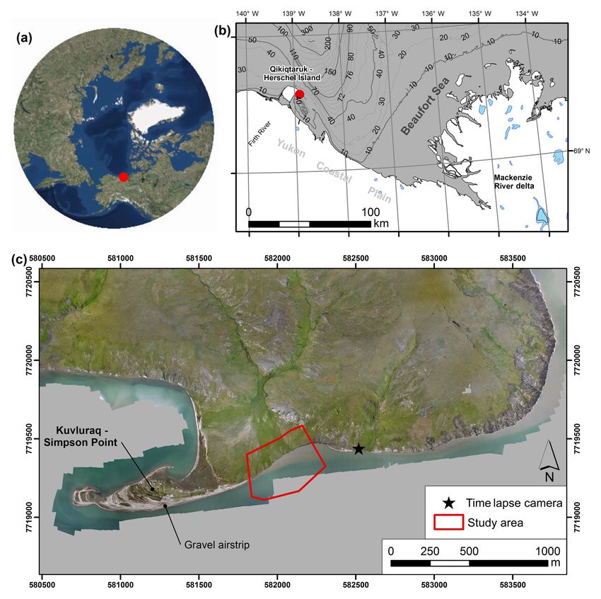
1514                                                      A. M. Cunliffe et al.: Drones observe eroding permafrost coastline

mafrost (Lantuit et al., 2012). Coastal erosion mobilises large       In this study, we used repeated drone surveys to investigate
amounts of sediment, organic matter, and nutrients from per-       short-term dynamics of an eroding permafrost coastline at
mafrost (Lantuit et al., 2012; Overduin et al., 2014; Reta-        Qikiqtaruk – Herschel Island (Yukon Territory) in the Cana-
mal et al., 2008; Wegner et al., 2015), which are released         dian Beaufort Sea across a 13-month period. We investigated
into the nearshore waters and affect marine ecosystems (Bell       what additional insights are available from observing shore-
et al., 2016; Dunton et al., 2006; Fritz et al., 2017). Sev-       line positions at fine spatial and temporal resolution, whether
eral studies have reported signs of accelerating coastal ero-      fine-resolution observations of shoreline change could be
sion rates at locations around the Arctic, including the west-     related to meteorological and oceanographic variables, and
ern Arctic (Barnhart et al., 2014; Jones et al., 2008, 2009b;      compared intra-seasonal shoreline change with historical
Mars and Houseknecht, 2007; Radosavljevic et al., 2016) and        shoreline changes over the last 65 years. For our study area,
Siberia (Günther et al., 2015; Kritsuk et al., 2014; Novikova      we hypothesise that the erosion of the observed permafrost
et al., 2018; Ogorodov et al., 2016). However, the spatio-         coastline adjacent to the settlement on Qikiqtaruk – Herschel
temporal resolution of circum-Arctic studies limits infer-         Island varies greatly between years and continuing erosion
ences of widespread changes in coastal erosion rates (Fritz        could threaten key infrastructure for human activities on the
et al., 2017). Erosion plays a critical role in the longer-term    island.
evolution of permafrost coastlines (Barnhart et al., 2014) and
biogeochemical cycling in coastal zones (Fritz et al., 2017;
Semiletov et al., 2016; Vonk et al., 2012), and the majority       2     Methods
of permafrost erosion studies compare multi-annual coastline
changes to infer annualised erosion rates over periods of sev-     2.1    Study site
eral years (Irrgang et al., 2018; Overduin et al., 2014). How-
ever, such coarse observation frequencies neglect the intra-       Qikiqtaruk – Herschel Island is located in the western Cana-
seasonal dynamics during the open-water season, including          dian Arctic in the Beaufort Sea (69◦ N, 139◦ W, Fig. 1a). The
episodic thaw and abrupt erosion events. Knowledge of these        island is an ice-thrust push moraine formed during the max-
intra-seasonal dynamics is essential to understand the pro-        imal advance of the Laurentide ice sheet (Fritz et al., 2012;
cesses and drivers controlling erosion patterns over time and      Pollard, 1990), and is underlain by ice-rich continuous per-
for better projecting future erosion rates in light of ongoing     mafrost (Brown et al., 1997; Lantuit and Pollard, 2008; Obu
Arctic changes (Obu et al., 2016; Vasiliev et al., 2005).          et al., 2016). Low spits composed of coarse material occur on
   The use of remote sensing to measure changes in per-            the east and west sides of the island (Couture et al., 2018).
mafrost landscapes is increasingly common (Novikova et             The mean annual air temperature is −11 ◦ C (1970–2000)
al., 2018). However, optical image coverage in high-latitude       and the mean annual precipitation is ca. 200 mm a−1 (Burn,
regions has historically been widely limited to relatively         2012). The average coastal erosion rate for the whole of
coarse temporal and spatial resolutions, due to frequent cloud     Qikiqtaruk – Herschel Island was 0.45 m a−1 between 1970
cover and logistical challenges that limit both satellite ob-      and 2000 (Lantuit and Pollard, 2005; Obu et al., 2015) and
servations and aerial surveys (Hope et al., 2004; Stow et          0.68 m a−1 between 2000 and 2011 (Obu et al., 2016).
al., 2004). Recently there has been a widespread interest in          Ice break-up typically commences in late June and open-
the use of lightweight drones, also known as remotely piloted      water conditions persist until early October (Dunton et
aerial systems or unmanned aerial vehicles (UAVs), to en-          al., 2006; Galley et al., 2016), although for Herschel Basin
able landscape managers and researchers to self-service their      and Thetis Bay land-fast sea ice can persist for longer pe-
data collection needs (Klemas, 2015; Westoby et al., 2012),        riods. The continental shelf in this part of the Beaufort Sea
thus democratising data acquisition (DeBell et al., 2015).         is very narrow and intersected by a deeper sea canyon, the
Lightweight drones combined with image-based modelling             Mackenzie Trough located north of Qikiqtaruk – Herschel Is-
can provide highly accurate and detailed measurements of           land (Dunton et al., 2006) (Fig. 1b). This area is microtidal,
rapidly changing features. These aerial observations can be        with a mean range of just 0.15 m for semidiurnal and monthly
obtained at user-determined frequencies (e.g. weekly, daily,       tides, but these are superimposed on a ca. 0.66 m annual
or even hourly if weather conditions permit), using rela-          tidal cycle, which peaks in late July (Barnhart et al., 2014;
tively inexpensive tools such as suitable multirotor drones        Huggett et al., 1975). The interaction between meteorologi-
available for less than USD 1000. Over the last few years,         cal factors including wind and wave action and coastal mor-
drone surveys are increasingly used for monitoring coastal         phology exerts more influence on water levels than tidal cy-
systems (Casella et al., 2016; Duffy et al., 2017b; Mancini        cles. The study area is characterised by dominant northwest-
et al., 2013; Turner et al., 2016). However, there have been       erly (NW) and prevailing easterly (E) winds. Northwesterly
very few examples of their application to monitor the ongo-        winds drive a positive storm surge and easterly winds drive a
ing rapid changes along permafrost coastlines (although see        negative surge at Qikiqtaruk – Herschel Island (Héquette et
Whalen, 2017; Whalen et al., 2017).                                al., 1995; Héquette and Barnes, 1990), with easterly winds
                                                                   also facilitating the transport of relatively warmer water dis-

The Cryosphere, 13, 1513–1528, 2019                                                    www.the-cryosphere.net/13/1513/2019/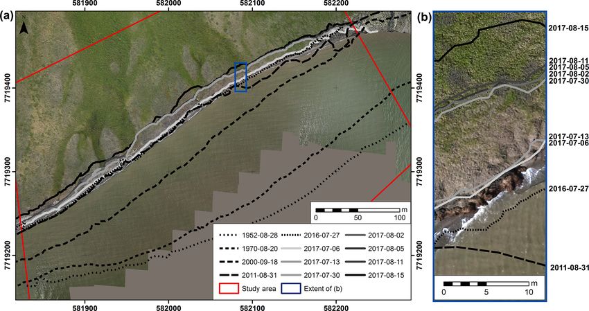
A. M. Cunliffe et al.: Drones observe eroding permafrost coastline                                                                1515

Figure 1. (a) The location of the study region in the western Canadian Arctic (basemap from ESRI et al., 2018, polar stereographic pro-
jection), (b) Qikiqtaruk – Herschel Island in the Beaufort Sea (shorelines from Wessel and Smith, 1996), and (c) true-colour orthomosaic
compiled from ca. 9000 individual images collected by drone survey in August 2017 indicating the location of the 500 m study stretch and
the time-lapse camera including viewing direction indicated by the camera symbol used to make Video S1 relative to Kuvluraq – Simpson
Point.

charged from the Mackenzie River towards the island (Dun-             are approximately −8 ◦ C (Burn and Zhang, 2009), and are
ton et al., 2006). The contemporary rate of relative sea level        known to be warming in recent decades (Burn and Zhang,
rise along this part of the Canadian Beaufort Sea is thought          2009; Myers-Smith et al., 2019). This study area lies entirely
to range between ca. 1.1 and 3.5 mm a−1 (James et al., 2014;          within the slightly larger “coastal reach 3” unit considered by
Manson et al., 2005).                                                 Radosavljevic et al. (2016), who reported coastal retreat rates
   This study focusses on a 500 m long coastal stretch located        of 1.4 ± 0.6, 1.7 ± 0.7, and 4.0 ± 1.1 m a−1 for the periods
to the east of Kuvluraq – Simpson Point, a coarse clastic             1952–1970, 1970–2000, and 2000–2011, respectively. For
spit (Fig. 1c). The study reach is along the edge of an al-           further details on the changing ecological and erosional con-
luvial fan, comprised of redeposited marine and glaciogenic           text of this site, see Burn (2012), Radosavljevic et al. (2016),
sediments that form Qikiqtaruk – Herschel Island (Fritz et            and Myers-Smith et al. (2019).
al., 2011; Rampton, 1982). The spit is attached to the alluvial          Coastal erosion at our study site threatens the human set-
fan, and is supplied by sediment from the alluvial fan and the        tlement and infrastructure on Qikiqtaruk – Herschel Island,
high bluffs to the east (Radosavljevic et al., 2016). The focal       located on Kuvluraq – Simpson Point (Olynyk, 2012; Ra-
coastline is characterised by low to moderately high bluffs           dosavljevic et al., 2016). This gravel spit bounds the natural
(ca. 1–5 m in elevation). Ice contents in these bluffs are high,      anchorage of Ilutaq – Pauline Cove, and is an important re-
at typically ca. 40 % ice by volume (Obu et al., 2016), which         gional hub for local and indigenous travellers, park admin-
is slightly lower than the typical 50 %–60 % ice content mod-         istration and rangers, tourists, and researchers in the western
elled for ice-thrust moraines along this portion of the Yukon         Canadian Arctic (e.g. Burn and Zhang, 2009; Myers-Smith
Coast (Couture and Pollard, 2017). Permafrost temperatures            et al., 2019). The currently seasonally inhabited settlement is

www.the-cryosphere.net/13/1513/2019/                                                         The Cryosphere, 13, 1513–1528, 2019
1516                                                      A. M. Cunliffe et al.: Drones observe eroding permafrost coastline

part of the Qikiqtaruk – Herschel Island Territorial Park, and     sion 1.3.3) (Agisoft, 2018; Sona et al., 2014), and process-
accommodates a number of culturally and historically sig-          ing parameters are reported in Table S1 in the Supplement.
nificant sites resulting in its candidature for UNESCO World       GNSS-derived geolocations for each individual image and
Heritage status (UNESCO, 2004). The proximity to the sea           the precisely geolocated ground control markers provided
and low elevation of this settlement at ≤ 1.2 m above sea          additional spatial constraint of the photogrammetric process-
level leads to high risk of coastal hazards, particularly flood-   ing (Carrivick et al., 2016; Cunliffe et al., 2016; Westoby
ing (Myers-Smith and Lehtonen, 2016; Olynyk, 2012; Ra-             et al., 2012). The photogrammetric processing yielded geo-
dosavljevic et al., 2016).                                         registered orthomosaic composite images and digital surface
                                                                   models. Note that the height field approaches to surface mod-
2.2    Drone and time-lapse image acquisition                      elling used in this analysis are not capable of capturing topo-
                                                                   graphic change related to the undercutting of bluffs. Captur-
In 2016, one drone survey was conducted in late July, fol-         ing such overhanging features with photogrammetric meth-
lowed by seven additional drone surveys over a 40 d pe-            ods can be possible, but requires optimising image acquisi-
riod between 6 July and 15 August 2017. Drone surveys              tion and more computationally intensive post-processing. To
were conducted using two platforms: (i) a lightweight flying-      inform qualitative interpretation of the erosion dynamics at
wing Zeta Phantom FX-61 with a Pixhawk flight controller           this location, a time-lapse camera was installed at the loca-
equipped with a Sony RX-100ii camera (100 CMOS sensor              tion indicated in Fig. 1, imaging the study coastline at hourly
with 20.2 megapixels) and (ii) a multi-rotor DJI Phantom 4         intervals for 4 d between 29 July and 3 August 2017.
Pro (100 CMOS sensor with 20 megapixels). Drone opera-
tions were conducted in accordance with an SFOC issued             2.3   Image alignment and shoreline mapping
by Transport Canada (to assist others seeking such permis-
sion, our full application is available at https://arcticdrones.   In addition to the drone surveys, we also used four “historic”
org/regulations/, last access: 10 May 2019). Black and white       panchromatic aerial photographs from 1952 and 1970, and
ground control markers were deployed along the shoreline           satellite images from 2000 and 2011 (previously analysed by
and precisely geolocated to an absolute accuracy of approx-        Radosavljevic et al., 2016). These four images had already
imately 0.02 m using real-time kinematic global navigation         been orthorectified in PCI OrthoEngine to minimise image
satellite system (GNSS) equipment (Leica Geosystems). We           distortion. We co-registered these four historic orthorectified
used between 3 and 132 markers in the surveys, depend-             images to the 6 July 2017 orthomosaic image in a geographic
ing on survey extents and destruction of markers by natu-          information system (ArcGIS, version 10.5, ESRI), as we con-
ral processes; ideally, we recommend using n = 13 ground           sidered this orthomosaic to have the best spatial constraint
control markers, distributed evenly across the area of interest    and coverage of all of the available datasets. All 12 images
(Carrivick et al., 2016; Cunliffe and Anderson, 2019). Image       were aligned to a common spatial framework: NAD83 UTM
overlap, a function of front-lap and side-lap, captured each       7N (EPSG: 26907). Further details of all images and compos-
part of the study area in at least five and usually > 10 pho-      ite orthomosaics are summarised in Table 1. Alignment er-
tographs; this equates to fore-/side-lap values of 56 % and        rors were estimated as the root-mean-square error (RMSE) of
69 %, respectively. For 2-D orthomosaics and 3-D elevation         the control points. While this approach to quantifying align-
models, we ideally recommend higher levels of overlap, ca.         ment error is standard practice in shoreline change analysis
8–10 and ca. 12–20 overlapping images, respectively. Drone         (Irrgang et al., 2018; Novikova et al., 2018; Río and Gra-
surveys over this study area had flight times of ca. 15–25 min,    cia, 2013), we note that the RMSE of control points is not a
at altitudes ranging from 30 to 120 m (Table 1). The geo-          strong metric of this uncertainty, as transformation parame-
tagged red–green–blue (RGB) photographs from each aerial           ters (georeferencing) and the intrinsic and extrinsic camera
survey had ground-sampling distances ranging from 10 to            parameters (structure-from-motion photogrammetry) are ad-
40 mm. Although this study presents drone surveys for a lim-       justed to minimise the RMSE. Consequently, for an indepen-
ited (500 m) extent of shoreline, drone surveys could be opti-     dent assessment of image registration error, in future work it
mised to observe larger reaches of up to ca. 1.5 to 2 km, par-     would be preferable to use the RMSE of independent check
ticularly in jurisdictions such as Canada where current regu-      points, which were not used to constrain transformation or
lations permit UAV operations up to 926 m from the remote          bundle adjustment parameters (James et al., 2017). Visual
pilot(s). For example, using two drones we found it possi-         comparison of each dataset indicated excellent spatial agree-
ble to survey over 8 km2 in a single day. Survey parameters        ment and suitability for further analysis (Jones et al., 2018).
including date and time of day, aircraft, altitude, and num-       Pixel error refers to the spatial resolution of the digital satel-
ber of ground control markers are given in Table 1. For fur-       lite and orthomosaic composite images, and for aerial pho-
ther discussion of recommended drone survey parameters for         tographs is a metric of image quality calculated based on the
different applications, see Carrivick et al. (2016) and Duffy      scale factor of each image multiplied by the typical resolu-
et al. (2017a). Drone images were processed with structure-        tion of a 9 × 9 in. aerial photogrammetric camera (after Ra-
from-motion photogrammetry using Agisoft PhotoScan (ver-           dosavljevic et al., 2016).

The Cryosphere, 13, 1513–1528, 2019                                                     www.the-cryosphere.net/13/1513/2019/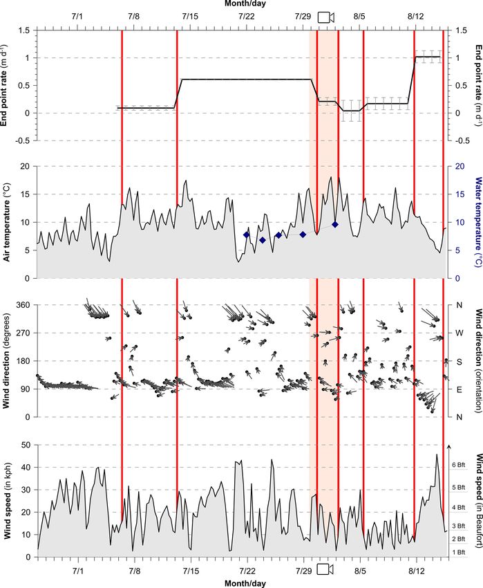
A. M. Cunliffe et al.: Drones observe eroding permafrost coastline 1517
Shorelines were digitised manually in ArcGIS for all 12
Table 1. Dataset and shoreline position parameters. The approximate times of drone surveys are in local time (UTC − 08:00). Total shoreline uncertainty is the root-mean-square error
images, at a scale of 1 : 600 for the four, older, coarser spa-
of (i) image co-registration (root-mean-square, rms, error of ground control points, GCPs), (ii) image quality (pixel error), and (ii) shoreline mapping (digitising) error (from Eq. 1).
tial resolution panchromatic images and a scale of 1 : 80
uncertainty (m)
Total shoreline
for the eight finer spatial resolution RGB orthomosaics. The
9.975
3.717
8.137
2.330
0.195
0.183
0.163
0.157
0.141
0.563
0.307
0.298
shoreline was defined as the vegetation edge rather than the
wet–dry line previously used in this region (Radosavljevic et
al., 2016) because the vegetation edge was both more visu-
ally distinct and temporally consistent than the wet–dry line
Digitising
error (m)
(Boak and Turner, 2005). Temporal consistency was essen-
4.00
2.00
2.00
1.50
0.15
0.10
0.10
0.10
0.10
0.10
0.15
0.10
tial to ensure meaningful assessment of coastal retreat over
short time intervals (Río and Gracia, 2013). Mapping shore-
line edges was possible with much greater fidelity on the
error(m)
fine-spatial-resolution RGB orthomosaic images compared
Pixel
3.50
0.60
1.00
0.50
0.03
0.02
0.02
0.02
0.02
0.02
0.04
0.02
to the coarser-spatial-resolution panchromatic images where
low contrast was sometimes an issue (Boak and Turner, 2005;
Río and Gracia, 2013). Shoreline digitising errors were esti-
Base image
mated by the GIS operator, and ranged between 0.1 and 4.0 m
Relative
Georeferencing
RMS error (m)
2.475
1.117
5.087
0.330
depending on image spatial resolution (Table 1).
–
–
–
–
–
–
–
2.4 Shoreline and elevation analysis
Absolute
(NAD83)
–
–
–
–
0.015
0.063
0.043
0.037
0.021
0.443
0.167
0.178
Total shoreline uncertainties were calculated as
U = EG + EP + ED , (1)
GCP
(n)
11
19
19
17
26
98
13
5
22
6
132
3
where U is total shoreline uncertainty, EG is georeferencing
error, EP is pixel error, and ED is digitising error (Table 1)
Scale
1 : 70 000
1 : 12 000
–
–
–
–
–
–
–
–
–
–
(Irrgang et al., 2018; Radosavljevic et al., 2016; Río and Gra-
cia, 2013). Additive error propagation is appropriate because
these error terms are not independent.
Shoreline position statistics were calculated with the
Images
(n)
1
1
1
1
317
1325
194
383
2040
336
8994
402
USGS Digital Shoreline Analysis System (DSAS version 4)
extension for ArcGIS (Thieler et al., 2009), using shore nor-
mal transects at 5 m intervals. Shoreline retreat rates in this
Altitude
(m)
120
120
120
31
100
37
120
42
study are given in end point rates for comparison between
surveys, and both end point rate and linear regression rate for
the entire time period of the study. The linear regression rate
RGB orthomosaic (Drone – Phantom)
RGB orthomosaic (Drone – Phantom)
RGB orthomosaic (Drone – Phantom)
RGB orthomosaic (Drone – Phantom)
uncertainty is the standard error of the slope parameter at the
Panchromatic IKONOS photograph
RGB orthomosaic (Drone – FX-61)
RGB orthomosaic (Drone – FX-61)
RGB orthomosaic (Drone – FX-61)
RGB orthomosaic (Drone – FX-61)
Panchromatic GeoEye photograph
95 % confidence interval. For further discussion on erosion
Panchromatic aerial photograph
Panchromatic aerial photograph
rate calculation, see Thieler et al. (2009). The accuracy of
shoreline change rates was calculated as
q
Ui2 + Uii2
DOA = , (2)
1t
Image type
where DOA is the dilution of accuracy (Dolan et al., 1991;
Himmelstoss et al., 2018; Irrgang et al., 2018), Ui is the total
shoreline uncertainty of the first point in time (from Table 1),
Uii is the total shoreline uncertainty of the shoreline posi-
tion from the second point in time, and 1t is the duration
11 Aug 2017 at 17:00
15 Aug 2017 at 10:20
2 Aug 2017 at 08:00
5 Aug 2017 at 11:40
13 Jul 2017 at 08:30
30 Jul 2017 at 18:00
6 Jul 2017 at 12:20
of the time period in years or days, as appropriate. Erosion
Observation date
rate errors refer to DOA values, unless otherwise stated, and
28 Aug 1952
20 Aug 1970
31 Aug 2011
18 Sep 2000
Table 2 displays the DOAs for all periods. We compared dif-
27 Jul 2016
ferences in modelled surface elevations between all periods
across a cross-sectional transect, and across the whole study
area for a 35 d period from 6 July to 11 August 2017 (dates
www.the-cryosphere.net/13/1513/2019/ The Cryosphere, 13, 1513–1528, 20191518 A. M. Cunliffe et al.: Drones observe eroding permafrost coastline
constrained by DSM quality as discussed below). During the illustrates the fluctuations in sea level and wave conditions
survey 6 July 2017, sea level was generally at −2.5 m relative and shows the undercutting, block failure, and denudation of
to the EPSG: 26907 datum. To exclude erroneous elevation detached blocks between 29 July and 3 August 2017.
observations from the sea, we digitised the water’s edge at a
scale of 1 : 80 and assigned a constant elevation of −2.5 m 3.2 Surface elevation change
to this seaward area. This approach excludes potential sub-
marine elevation change from the subsequent volume calcu- We generated digital surface models (DSM) of the coastal
lations. The volume of material eroded was calculated with topography from all eight photogrammetric surveys under-
the surface volume tool in ArcMap. taken in 2016 and 2017, spanning a 13-month period (Fig. 4).
However, in several cases, the DSMs did not yield reliable
2.5 Meteorological and oceanographic observations data across the entire coastal reach, due to insufficient spatial
constraint of the photogrammetric reconstructions. This issue
Meteorological observations were obtained from an Environ- was due in part to the destruction of ground control mark-
ment Canada weather station located on Kuvluraq – Simpson ers by faster-than-anticipated coastal retreat, as well as sub-
Point (station ID: “Herschel Island”, World Meteorological optimal distribution of GCPs and insufficient image overlap
Organisation ID: 71501; downloaded from http://climate. from some surveys due to weather constraints. Over the 35 d
weather.gc.ca/historical_data/search_historic_data_e.html, between two well-constrained DSMs from 6 July and 11 Au-
last access: 1 March 2018), and processed to extract mean 6 h gust 2017, ca. 28 m3 m−1 of material was removed (totalling
air temperature, wind speed, and wind direction throughout ca. 13 800 m3 across the 500 m coastline), at an average rate
the 2017 observation period. Conductivity–temperature– of ca. 0.79 m3 m−1 d−1 (Fig. 4a). These estimates do not in-
depth (CTD) profiles (see Fig. S2) were collected in July and clude the 4.1 ± 1.1 retreat observed between 11 and 15 Au-
August 2017 with a CastAway CTD (SonTek, USA) from gust. During this 4 d period, a further ca. 5300 m3 of ma-
a small research vessel ca. 1 km from the study area (near terial was probably removed (ca. 2.7 m3 m−1 d−1 ), assum-
69.552◦ N, 138.923◦ W). ing an average cliff height of 2.65 m as measured across
the preceding 35 d. Combined, this resulted in an estimated
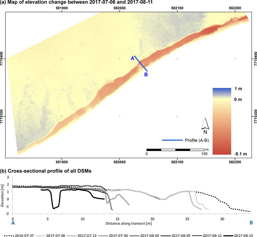
3 Results 19 100 m3 of material being removed over the 40 d. The el-
evation change map (Fig. 4a) illustrates the increase in bluff
3.1 Shoreline position analysis elevation from ca. 1 m in the west to ca. 5 m east across the
coastal reach. Inland of the shoreline, there were scattered
Over our observational period of 1952 to 2017, the coast- small increases in surface elevation, typically on the order of
line along the study reach retreated by an average of 143.7 ± 0.1–0.2 m; these might relate to the development (esp. leafing
28.4 m (where ± is the standard deviation of observations out) of tundra vegetation during the short summer growing
from each transect). The overall retreat rate was 2.2 ± season (Myers-Smith et al., 2019). In the centre of the study
0.1 m a−1 as calculated by end point rate and 1.9 ± 0.5 m a−1 reach, the DSMs were of sufficient quality to allow cross-
as calculated by the linear regression rate. Average retreat sectional comparisons across a ca. 3 m high bluff shown in
rates over decadal periods ranged between 0.7 ± 0.3 and Fig. 4b; these cross sections were sampled across the A–B
3.0±0.5 m a−1 . The net shoreline change and end point rates transect indicated in Figs. 3 and 4a. The depression in the
for all periods are presented in Table 2. 15 August 2017 elevation profile corresponds with the ca.
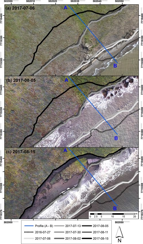
Over a 40 d period in the summer of 2017, shoreline re- 1 m gap behind a detached block, depicted in Fig. 3c, illus-
treat was 14.5 ± 3.2 m, ranging between 21.8 and 6.1 m, at trating the sensitivity of the surface elevation models.
an average rate of 0.36 m d−1 . The observed shoreline posi-
tions are depicted in Figs. 2 and 3, although the high tempo- 3.3 Meteorological, oceanographic, and time-lapse
ral frequency of observations throughout the summer of 2017 video observations
and episodic pattern of retreat meant that the shorelines were
sometimes very close in space. Most of the coastline retreat Erosion rates for each observation period through the sum-
occurred over two periods: (i) 27 d between 13 and 30 July mer of 2017 were compared to meteorological and oceano-
and (ii) 4 d between 11 and 15 August (Figs. 2, 3, and 5, Ta- graphic conditions, in order to better describe the controls on
ble 2). There was minimal change in coastline position dur- episodic and rapid erosion of this coastline (Fig. 5). From 3
ing the 6 d between 5 and 11 August, the 7 d between 6 and to 10 d prior to the first 2017 survey (on 6 July 2017), winds
13 July, and the 6 d between 30 July and 5 August (Fig. 2, Ta- were consistently strong from the east and their 6 h average
ble 2). The erosion at this coastline over 4 d is illustrated in speed reached up to 40 km h−1 (Fig. 5). For 0 to 3 d prior to
a time-lapse video (Video S1 in the Supplement). This cam- the same survey the dominant wind direction shifted to the
era was orientated facing west by southwest (Fig. 1) with the northwest with strong winds up to 40 km h−1 (Fig. 5), which
alluvial fan and the eroding cliff in the foreground and the raised the water level and refracted waves around the bluffs
structures of the settlement in the background. This video at Collinson Head to the northeast of the study reach. Over
The Cryosphere, 13, 1513–1528, 2019 www.the-cryosphere.net/13/1513/2019/A. M. Cunliffe et al.: Drones observe eroding permafrost coastline 1519
Table 2. Summary of shoreline change for all periods, in terms of net shoreline change and end point rates. Net shoreline change mean is the
distance between the oldest and youngest shorelines, where SD is standard deviation. End point rate is the net shoreline change normalised
by time (years or days, for supra- or sub-annual periods, respectively), where DOA is dilution of accuracy (after Eq. 2).
Period Days Mean net shoreline Mean end point
change ± SD rate ± DOA
(m) (m a−1 ) (m d−1 )
Supra-annual periods
28 Aug 1952–20 Aug 1970 6567 20.7 ± 10.6 1.2 ± 0.6
20 Aug 1970–18 Sep 2000 10 986 69.2 ± 21.9 2.3 ± 0.3
18 Sep 2000–31 Aug 2011 3986 33.0 ± 11.1 3.0 ± 0.8
31 Aug 2011–27 Jul 2016 1791 3.5 ± 4.6 0.7 ± 0.5
27 Jul 2016–6 Jul 2017 344 2.9 ± 2.2 3.1 ± 0.3
28 Aug 1952–15 Aug 2017 23 735 143.7 ± 28.4 2.2 ± 0.2 < 0.01 ± 0.00
Sub-annual periods
6–13 Jul 2017 7 0.5 ± 0.5 0.09 ± 0.04
13–30 Jul 2017 17 7.4 ± 5.6 0.61 ± 0.01
30 Jul–2 Aug 2017 3 0.6 ± 1.1 0.21 ± 0.07
2–5 Aug 2017 3 0.1 ± 0.4 0.04 ± 0.19
5–11 Aug 2017 6 1.0 ± 0.4 0.17 ± 0.11
11–15 Aug 2017 4 4.1 ± 1.1 1.02 ± 0.11
6–15 Aug 2017 40 14.5 ± 3.2 0.36 ± 0.01
Figure 2. (a) Overview of the 500 m study area, illustrating all 12 shoreline positions since 1952 overlaid on the 6 July 2017 orthomosaic.
(b) A 10-fold magnification in scale, illustrating the episodic nature of the shoreline changes at this location within the area of the blue
bounding box depicted in (a).
the 7 d between 6 and 13 July 2017, winds were predomi- table periods of very high-strength winds (ca. 40 km h−1 for
nantly from the southeast, with brief periods of strong winds 24 and 12 h, respectively) (Fig. 5), and surface water tem-
(ca. 30 km h−1 over 6 h) from the northwest (Fig. 5). These peratures reached nearly 10 ◦ C (see Fig. S3, CTD profile d).
meteorological conditions generally promoted waves from These conditions combined to drive rapid erosion, resulting
the southeast, which eroded the exposed cliff base (Figs. 4 in 7.4 ± 5.6 m (SD) of shoreline retreat in just 17 d (Figs. 3
and 5). Over the 17 d between 13 and 30 July, winds were and 4).
variable, but predominantly from the southeast, with two no-
www.the-cryosphere.net/13/1513/2019/ The Cryosphere, 13, 1513–1528, 20191520 A. M. Cunliffe et al.: Drones observe eroding permafrost coastline
dercutting that drove 4.1 ± 1.1 m (SD) of shoreline retreat in
just 4 d, largely through block failure (Figs. 3, 4, and S4, Ta-
ble 2). Sea surface temperatures were relatively warm at 6–
10 ◦ C when measured between 21 July and 2 August (Figs. 5,
S2). Figure S1 in the Supplement summarises wind vectors
and velocities observed during the summer of 2017.
4 Discussion
4.1 Rapid shoreline change
Over the 65-year record from 1952 to 2017, we found sub-
stantial erosion along the 500 m study coastline of Qikiqtaruk
– Herschel Island. The average rate of retreat was 2.2 m a−1 ,
ranging over decadal periods from 0.7 to 3.0 m a−1 (Table 2).
This long-term retreat rate is fast compared with 0.7 m a−1
for the Yukon coast (Irrgang et al., 2018), 1.1 m a−1 for the
Canadian Beaufort Sea (Lantuit et al., 2012), and circum-
Arctic observations where rates are typically between 0 and
2 m a−1 (Overduin et al., 2014) with a weighted mean of
0.57 m a−1 (Lantuit et al., 2012). Our study reach lies within
the slightly larger coastal reach 3 unit considered by Ra-
dosavljevic et al. (2016); consequently, differences in reach
length and historic image co-registration result in some slight
differences between the erosion rates reported herein and
those previously reported for the historic imagery. Coastal
retreat rates in the neighbouring Alaskan Beaufort Sea were
typically 0.7 to 2.4 m a−1 depending on coast type (Jorgen-
son and Brown, 2005), with extremes of up to 25 m a−1
(Jones et al., 2009b). Yet, the Alaskan Beaufort Sea coastline
is more similar to the western formerly non-glaciated part
of the Yukon Coast, with low cliffs, overall strong erosion
rates, and longer sea ice cover (Irrgang et al., 2018; Jorgen-
son and Brown, 2005; Ping et al., 2011). This is quite differ-
Figure 3. Shoreline positions between 2016 and 2017 overlaid on ent from our study coastline in the formerly glaciated part of
three orthomosaics for part of the study reach. The blocks shown the Yukon Coast (Rampton, 1982), which is characterised by
in (c) were detached from the bluff, with water moving freely be- high cliffs and high ground ice contents due to former move-
hind during periods of higher water level (see Fig. S3). Profile A–B ment and burial of glacier ice (Couture and Pollard, 2017;
indicates the horizontal position of the cross-sectional profiles dis- Fritz et al., 2011). Furthermore, the sea-ice-free season in our
cussed in Sect. 4.2 and depicted in Fig. 4. study area is longer than further west along the Alaskan coast
due to the warming influence of the Mackenzie River, but in
turn is modulated by the break-up of land-fast ice, which can
Over the 6 d between 30 July and 5 August, winds were be persistent in Herschel Basin and Thetis Bay (Dunton et
variable in direction and typically weaker (Fig. 5). This re- al., 2006). Erosion rates from linear regression tend to un-
sulted in minimal shoreline retreat (Table 2), but did remove derestimate rates calculated from end point reports (Dolan
cliff debris from the beach, facilitating further undercutting et al., 1991; Radosavljevic et al., 2016), which is consistent
(Video S1, Fig. 4). Over the 6 d between 5 and 11 August, the with our findings of 1.9 m a−1 vs. 2.2 m a−1 , but both linear
wind direction was variable and wind speed was low (6 h av- regression and end point rates alone do not account for un-
erages mostly below 20 km h−1 ), with relatively slow coast- certainty in shoreline positions (Himmelstoss et al., 2018).
line retreat of ca. 0.17 m d−1 . Over the 4 d between 11 and Changes in the rate of mean shoreline position for all time
15 August, a larger storm event developed, with wind shifting points are shown in Fig. S4.
from east through north to west and wind speeds increasing Over a 384 d period from 27 July 2016 to 15 August 2017,
to above 45 km h−1 for more than 6 h (Fig. 5). These mete- we observed a large retreat in the shoreline position, with
orological conditions generated large waves and caused un- an average of 17.4 m, although note that this period is 19 d
The Cryosphere, 13, 1513–1528, 2019 www.the-cryosphere.net/13/1513/2019/A. M. Cunliffe et al.: Drones observe eroding permafrost coastline 1521 Figure 4. (a) Map of elevation change in digital surface models between 6 July and 11 August 2017, illustrating areas of erosion along the coastline with up to −5.1 m of change and also some minor (ca. 0.1 m) increases inland that we attribute to vegetation development. (b) Elevation profiles along the A–B transect shown in (a) and Fig. 3, extracted from digital surface models (no vertical exaggeration). Note that two of the latter elevation models (from 8 and 15 August 2017) both suffered from datum problems due to insufficient spatial constraint; see discussion for details. longer than a year and includes a disproportionate number of of the bluff following cliff failure, thus reducing protection days from the open-water season. Most of this rapid retreat of the bluff base from further wave action (Héquette and occurred in the summer of 2017, when we measured 14.5 m Barnes, 1990). Given the episodic nature of coastal retreat, it of coastline retreat over just 40 d. Our own qualitative obser- can be difficult to compare short-term rate changes with long- vations on the ground over the summer of 2017 (Video S1) term observation periods (< 2 vs. > 10 years, respectively) confirmed the extremely rapid shoreline changes reported (Dolan et al., 1991). However, to remain consistent with the above. In this time, we estimate approximately 19 000 m3 long-term average rate of 2.2 m a−1 , no further erosion of this of material was eroded at a rate of ca. 0.96 m3 m d−1 . The coastline would need to occur for more than 7 years after the coastal erosion processes we observed during 40 d of 2017 retreat observed in 2016 and 2017. correspond with the conceptual model described by Barn- The rapid coastline retreat observed in this study reach is hart et al. (2014) (Video S1 and Fig. S3). The bluffs along consistent with, but greater than, earlier analysis of neigh- the alluvial fan were affected by thermo-denudation but par- bouring coastal reaches on Qikiqtaruk – Herschel Island be- ticularly thermo-abrasion due to the combined mechanical tween 1952 and 2011 (Radosavljevic et al., 2016) and also and thermal action of seawater, causing undercutting and coastal retreat observed in other Arctic permafrost coast- subsequent block failure (Barnhart et al., 2014; Günther et lines (Günther et al., 2013; Irrgang et al., 2018; Jones et al., 2012; Vasiliev et al., 2005). These thermal processes are al., 2009a; Whalen et al., 2017). Coastline retreat rates al- likely influenced by warm surface waters delivered from the most doubled from 7.6 m a−1 (1955–2009) to 13.8 m a−1 Mackenzie River delta during easterly wind conditions (Dun- (2007–2009) at Cape Halkett on the Alaskan Beaufort Sea ton et al., 2006). Additional factors facilitating rapid erosion (Jones et al., 2009a), and more than doubled from 2.2 m a−1 at this site are the high ice content (ca. 40 % Obu et al., 2016) (1952–2010) to 5.3 m a−1 (2010–2012) on Bykovsky Penin- and the low relief, as less material is deposited at the base sula, Siberia (Günther et al., 2013). Increases in erosion rates www.the-cryosphere.net/13/1513/2019/ The Cryosphere, 13, 1513–1528, 2019
1522                                                         A. M. Cunliffe et al.: Drones observe eroding permafrost coastline

Figure 5. Shoreline retreat (end point) rates normalised by day for each observation period in 2017, 6 h moving averages of air temperature,
wind direction, and wind velocity in July–August 2017 (data from Environment Canada, 2017). Dates and times of aerial surveys are indicated
by the red bars, point measurements of sea surface temperature from CTD casts are indicated by blue diamonds (see Fig. S3 for full CTD
profiles), and the duration of time-lapse survey shown in Video S1 is indicated by the red shading.

greater than 2-fold are more commonly observed on low-                  changes at near-annual temporal resolution, considering a
elevation coasts, such as the one examined herein and in                larger range of representative coastal reaches and study sites.
Jones et al. (2009a). On the Yukon Coast, average coastal re-
treat rates were 0.5 m a−1 between 1950 and 1970 (Harper et             4.2    Drivers of rapid shoreline change
al., 1985) and 0.7 m a−1 between 1950 and 2011 (Irrgang et
al., 2018), with maximum reported rates of 22 m a−1 on Pelly            The rapid retreat observed in 2016 and especially 2017 was
Island (NWT) 130 km to the east along the Yukon–NWT                     likely driven by a range of factors, including longer-term
coast (Whalen et al., 2017). Robustly detecting changes in              conditioning factors acting over timescales of decades to
the trends of permafrost coastline erosion in this region and           years and also shorter-term factors acting over timescales
more widely requires further analyses of shoreline position             of weeks to days and hours. Over the longer term, this
                                                                        region experiences a relative sea level rise of ca. 1.1 to

The Cryosphere, 13, 1513–1528, 2019                                                           www.the-cryosphere.net/13/1513/2019/
A. M. Cunliffe et al.: Drones observe eroding permafrost coastline 1523 3.5 mm a−1 (James et al., 2014; Manson et al., 2005), pro- two periods with the most rapid erosion in 2017 (the 27 d be- gressively subjecting more permafrost to thermo-abrasional tween 13 and 30 July and the 4 d between 11 and 15 August) processes. Seasonal sea ice break-up has advanced earlier by were both associated with strong winds (6 h moving aver- 46 d per decade between 2002 and 2016 (Assmann, 2019), ages exceeding > 40 km h−1 ), both easterly and northwest- with ice-free seasons lengthening by 9 d per decade between erly, and preceded by relatively high air and water tempera- 1979 and 2013 (Stroeve et al., 2014) and summer minimum tures (Fig. 5). Together, these conditions likely enhanced the sea ice concentrations decreasing over the last 39 years in thermo-abrasional processes undercutting the ice-rich bluff. this area (Myers-Smith et al., 2019). This region is gener- The high temporal frequency of shoreline position observa- ally experiencing longer open-water seasons and increasing tions is essential to studying highly episodic erosion pro- wave heights (Barnhart et al., 2014; Farquharson et al., 2018; cesses. For example, ca. 30 % (4.2 m) of the 14.5 m of shore- Stroeve et al., 2014), and there is increased heat influx to the line retreat in the summer of 2017 happened in just 4 d (11– ocean during the open-water season, due to increasing dis- 15 August), indicating discrete storm events can play a ma- charge from the Mackenzie River and atmospheric warm- jor role in the geomorphic development of permafrost shore- ing. Atmospheric warming has increased permafrost tem- lines (Farquharson et al., 2018; Solomon et al., 1993). Fu- peratures and deepened the active layer at sites just 1 km ture work relating coastline change to meteorological and from the study reach (Burn and Zhang, 2009; Myers-Smith oceanographic factors over short timescales will need to et al., 2019), lowering the energy required to thaw the per- consider the latencies involved between meteorological and mafrost, although lengthening open-water seasons is likely oceanographic conditions, undercutting of permafrost cliffs, to be the most significant factor (Farquharson et al., 2018). and planform change as observed from an aerial perspective. Attribution of the rapid change in shoreline position in 2017 to a single main driver is not possible with the avail- 4.3 Rapid coastal erosion as potential threat for the able datasets. Examination of MODIS observations indicates Territorial Parks infrastructure sea ice break-up was ca. 15 d earlier in 2015 and 2016, but in 2017 it was in line with the 10-year average (Fig. S5). Coastal change near the Ilutaq – Pauline Cove area influ- The direction and frequency of wind patterns observed in ences the stability and evolution of the adjacent gravel spit, 2017 (Figs. 5, S1) are similar to those reported in June– which accommodates culturally and historically significant September from 2009 to 2012 (Radosavljevic et al., 2016, sites, as well as infrastructure essential to the operation of Fig. 4 therein). However, overall wind speeds were higher in the Qikiqtaruk – Herschel Island Territorial Park. Shoreline 2017, with a greater proportion of periods with mean speeds change and flooding in recent history has already necessi- in excess of > 30 km h−1 (Fig. S1). The role of wind is dis- tated the relocation and raising of several historic buildings cussed further below. A large portion of beach and cliff debris at the Ilutaq – Pauline Cove settlement, as well as the reloca- appeared to have been removed between our survey in 2016 tion of the gravel airstrip essential to the operation of the park (26 July 2016) and our first survey in 2017 (6 July 2017) (Olynyk, 2012). However relocation efforts are hindered by (Fig. 4b, and corroborated by our field observations), poten- the fragility of several buildings, particularly the “Commu- tially either during storm events in the autumn of 2016 and/or nity House”, the oldest building in the Yukon, and it is in- ice bulldozing during ice break-up in spring 2017. We hy- creasingly difficult to find safer locations for these buildings pothesise that removal of this protective material may have on the spit (Olynyk, 2012). These historic buildings underpin increased the susceptibility of these cliffs to rapid erosion in the site’s candidature for UNESCO status (UNESCO, 2004). the summer of 2017. Field observations from 2018 suggest Erosion of the observed coastal reach exposes the base of the that the shoreline retreat has stabilised at rates closer to the spit to coastal processes, increasing the risk of changes to long-term average. the position of the spit itself. Flooding during storm events Through the summer of 2017, coastal retreat was highly can isolate the spit from the island (Myers-Smith and Lehto- episodic. The main mode of erosion was block failure fol- nen, 2016), and such events are projected to become more lowing thermo-abrasional undercutting. This undercutting common in the future (Radosavljevic et al., 2016). Knowl- appeared to be largely influenced by fluctuations in wa- edge of coastal processes, particularly patterns of contempo- ter level combined with wave action. Water level fluctua- rary coastal retreat as a proxy for future patterns, is therefore tions appeared to be mainly determined by wind-generated valuable for informing local management decisions. surges and waves, superimposed on tidal patterns (Héquette et al., 1995; Héquette and Barnes, 1990). Although this re- 4.4 Using drones to quantify fine-scale coastal erosion gion is microtidal, with a mean range of just 0.15 m for dynamics semidiurnal and monthly tides, these are superimposed on a ca. 0.66 m annual tidal cycle which peaks in late July (Barn- Drone surveys and photogrammetric analysis are effective hart et al., 2014), corresponding with our intensive observa- tools for measuring fine-scale erosion dynamics along per- tion period. Annual tides therefore likely influence the timing mafrost coastlines, yielding orthomosaics, inferred shore- of coastal retreat within the ice-free season in this area. The line positions (Figs. 2 and 3), and surface elevation models www.the-cryosphere.net/13/1513/2019/ The Cryosphere, 13, 1513–1528, 2019
1524                                                      A. M. Cunliffe et al.: Drones observe eroding permafrost coastline

(Fig. 4). When supplemented by other monitoring of envi-           optimising placement of ground control, see Carrivick et
ronmental variables (such as wave fields, sea surface tem-         al. (2016) and James et al. (2017).
perature, wind strength and direction), drone-acquired ob-
servations at fine spatio-temporal resolutions can be related
to meteorological and oceanographic observations on supra-
annual timescales, providing quantitative insights into ero-       5   Conclusion
sion processes that vary greatly in time and space. The tem-
poral resolution of drone surveys can greatly exceed those         We used drones as a highly effective instrument to observe
available by more traditional forms of remote sensing, for ex-     the dynamics of permafrost coastline changes associated
ample satellite observations or surveys from manned aircraft       with supra-seasonal erosion on Qikiqtaruk – Herschel Is-
(Casella et al., 2016; Stow et al., 2004; Whalen et al., 2017),    land. In 2017, average shoreline retreat was extremely rapid
and such observations can be more informative than previ-          at 14.5 m over 40 d, well in excess of the long-term average
ously available proxies (such as the apparent cross-sectional      of 2.2 m a−1 from 1952 to 2017. The volume of material re-
area of detached blocks; Barnhart et al., 2014). Such spa-         moved was ca. 0.96 m3 m d−1 in 2017. A total of 30 % of the
tial observations could be used to robustly evaluate and re-       rapid 2017 shoreline change (4.1 m retreat) occurred in just
fine process-based numerical models of coastal erosion over        4 d during one storm event. Block failure was the prevail-
multiple temporal scales (Barnhart et al., 2014; Casella et        ing mode of erosion, seemingly driven by multiple factors
al., 2014; Wobus et al., 2011).                                    that increase the susceptibility of the permafrost coastline to
   Lightweight drones can be deployed at a relatively low          thermo-abrasional processes. These rapid erosion events ob-
cost when suitably trained and equipped personnel are on           served on Qikiqtaruk – Herschel Island appear to have been
site. However, the costs of accessing high-latitude sites can      driven by short-term fluctuations in water levels due to mete-
be substantial, potentially contributing to uneven distribu-       orological conditions, possibly superimposed on annual tidal
tions of monitoring sites (Metcalfe et al., 2018). Surveyable      cycles on a longer-term background of relative sea level rise
spatial extents depend on the size and the range of the re-        and increasing heat flux from the Mackenzie River discharge
motely piloted drone, and are also limited by safety and reg-      and the atmosphere.
ulatory restrictions. Observations from optical satellites may        We found that lightweight drones and aerial photogram-
be better suited for observing change across larger sections       metry can be cost-effective tools to capture short-term coastal
of coastline; however, high levels of cloud cover in Arctic        erosion dynamics and related shoreline changes along dis-
regions limit the frequency of successful optical satellite ob-    crete sections of permafrost coasts. At our study site on Qik-
servations (Hope et al., 2004; Stow et al., 2004). Continu-        iqtaruk – Herschel Island further erosion and removal of this
ing advances in satellite sensors have increased the spatial       coastal reach could threaten the infrastructure of the settle-
resolution and revisit frequency of observations, yet freely       ment over the long term. With the rapid maturation of drone
available products are currently only available for spatial res-   platforms and image-based modelling technologies, these ap-
olutions of ca. ≥ 10 m (e.g. Sentinel 2), and finer-spatial-       proaches can now be easily deployed at both supra- and sub-
resolution (< 4 m) products have non-trivial costs for each        annual timescales to obtain new insights into coastal ero-
scene.                                                             sion and inform management decisions. These approaches
   In summary, lightweight drone surveys can be suitable           are particularly relevant in permafrost coastlines, where ero-
when there is a need to accurately measure small changes           sion can be highly episodic, with long-term rates dominated
(e.g. ≤ 0.3 m) in shoreline positions or elevations over lim-      by short-term events. By combining new methods of obser-
ited extents (e.g. ≤ 5–10 km in length). Fine-resolution mea-      vation with long-term records, we can improve predictions
surements from drone products will be especially useful for        of coastal erosion dynamics and subsequent consequences
isolating the drivers of coastal erosion events, and contin-       for the management of fragile Arctic coastal ecosystems and
ued miniaturisation of thermal and multispectral cameras for       cultural sites.
drone platforms will create opportunities to better understand
these mechanisms of change. Measurements of surface el-
evation and consequently volume change can be more in-             Data availability. The georectified aerial images underpinning this
                                                                   analysis are available for download from PANGAEA (https://doi.
formative than simple 2-D representations of shoreline po-
                                                                   pangaea.de/10.1594/PANGAEA.901852, Cunliffe et al., 2019). The
sition. We generated digital surface models following our          digital elevation models are available from the corresponding author
drive surveys; however, issues with insufficient spatial con-      upon request. Meteorological observations are available from Envi-
straint meant that full area coverage was only possible from       ronment Canada.
some of the surveys. If elevation observations are required,
care should be taken when conducting drone surveys to en-
sure that there will be sufficient spatial constraint of the       Video supplement. A supplementary time-lapse video of the coastal
photogrammetric modelling process, even if coastal retreat         erosion reported here is available at https://doi.org/10.5446/40250
is faster than expected. For further recommendations on            (Cunliffe et al., 2017).

The Cryosphere, 13, 1513–1528, 2019                                                     www.the-cryosphere.net/13/1513/2019/
A. M. Cunliffe et al.: Drones observe eroding permafrost coastline 1525
Supplement. The supplement related to this article is available fort Sea shelf and slope, Mar. Ecol. Prog. Ser., 550, 1–24,
online at: https://doi.org/10.5194/tc-13-1513-2019-supplement. https://doi.org/10.3354/meps11725, 2016.
Boak, E. H. and Turner, I. L.: Shoreline definition and
detection: a review, J. Coastal Res., 2005, 688–703,
Author contributions. AMC and GT contributed equally to this https://doi.org/10.2112/03-0071.1, 2005.
work. Conceptualisation, AMC, GT, JTK and IHM-S; Data cura- Brown, J., Ferrians Jr., O. J., Heginbottom, J. A., and Melnikov,
tion, AMC; Formal analysis, AMC and GT; Funding acquisition, E. S.: Circum-Arctic map of permafrost and ground-ice condi-
IHM-S, TS, and HL; Investigation, AMC, GT, BR, WFP and JTK; tions, USGS Numbered Series, available at: http://pubs.er.usgs.
Methodology, AMC; Project administration, AMC; Supervision, gov/publication/cp45 (last access: 9 April 2018), 1997.
TS, HL and IHM-S; Visualisation, AMC, GT and WFP; Writing Burn, C. R.: Herschel Island Qikiqtaryuk: A Natural and Cultural
– original draft, AMC; Writing – review & editing, AMC, GT, BR, History of Yukon’s Arctic Island, 1st edn., Calgary University
WFP, TS, HL, JTK and IHM-S. Press, Calgary, Canada, 2012.
Burn, C. R. and Zhang, Y.: Permafrost and climate change at Her-
schel Island (Qikiqtaruq), Yukon Territory, Canada, J. Geophys.
Competing interests. The authors declare that they have no conflict Res., 114, F02001, https://doi.org/10.1029/2008JF001087, 2009.
of interest. The funding sponsors had no role in the design of the Carrivick, J. L., Smith, M. W., and Quincey, D. J.: Structure from
study; in the collection, analyses, or interpretation of data; in the Motion in the Geosciences, John Wiley & Sons, Ltd, Chichester,
writing of the paper; or in the decision to publish the results. UK, 2016.
Casella, E., Rovere, A., Pedroncini, A., Mucerino, L.,
Casella, M., Cusati, L. A., Vacchi, M., Ferrari, M., and
Firpo, M.: Study of wave runup using numerical mod-
Acknowledgements. We wish to thank the Qikiqtaruk Territorial
els and low-altitude aerial photogrammetry: A tool for
Park staff including Richard Gordon, Edward McLeod, Samuel
coastal management, Estuar. Coast. Shelf S., 149, 160–167,
McLeod, Ricky Joe, Paden Lennie, and Shane Goesen, as well as
https://doi.org/10.1016/j.ecss.2014.08.012, 2014.
the Yukon government and Yukon parks for their permission and
Casella, E., Rovere, A., Pedroncini, A., Stark, C. P., Casella, M.,
support of this research (permit number Inu0216). We also thank
Ferrari, M., and Firpo, M.: Drones as tools for monitoring beach
the Inuvialuit people for their permission to work on their traditional
topography changes in the Ligurian Sea (NW Mediterranean),
lands. Drone flight operations were authorised by a Special Flight
Geo-Mar. Lett., 36, 151–163, https://doi.org/10.1007/s00367-
Operations Certificate granted by Transport Canada. We thank To-
016-0435-9, 2016.
bias Bolch, James Duffy, and the anonymous reviewers for insight-
Couture, N. J. and Pollard, W. H.: A Model for Quantifying Ground-
ful feedback that helped us to refine earlier versions of this paper.
Ice Volume, Yukon Coast, Western Arctic Canada, Permafrost
Periglac., 28, 534–542, https://doi.org/10.1002/ppp.1952, 2017.
Couture, N. J., Irrgang, A., Pollard, W., Lantuit, H., and Fritz,
Financial support. This research has been supported by the Natural M.: Coastal Erosion of Permafrost Soils Along the Yukon
Environment Research Council (grant no. NE/M016323/1), the Na- Coastal Plain and Fluxes of Organic Carbon to the Cana-
tional Geographic Society (grant no. CP-061R-17), the Helmholtz dian Beaufort Sea, J. Geophys. Res.-Biogeo., 123, 406–422,
Young Investigators Group “COPER” (grant no. VH NG 801), the https://doi.org/10.1002/2017JG004166, 2018.
Horizon 2020 (grant Nunataryuk (773421)), and the NERC Geo- Cunliffe, A. and Anderson, K.: Measuring Above-ground Biomass
physical Equipment Facility (grant nos. GEF:1063 and GEF:1069). with Drone Photogrammetry: Data Collection Protocol, Protocol
Exchange, https://doi.org/10.1038/protex.2018.134, 2019.
Cunliffe, A., Palmer, W., and Tanski, G.: Timelapse Video
Review statement. This paper was edited by Tobias Bolch and re- of Eroding Permafrost Coastline, Copernicus Publications,
viewed by two anonymous referees. https://doi.org/10.5446/40250, 2017.
Cunliffe, A. M., Brazier, R. E., and Anderson, K.: Ultra-
fine grain landscape-scale quantification of dryland veg-
etation structure with drone-acquired structure-from-motion
photogrammetry, Remote Sens. Environ., 183, 129–143,
References https://doi.org/10.1016/j.rse.2016.05.019, 2016.
Cunliffe, A. M., Tanski, G., Radosavljevic, B., Palmer, W.,
Agisoft: Agisoft PhotoScan User Manual: Professional Edition, Sachs, T., Kerby, J. T., and Myers-Smith, I. H .: Aerial im-
Version 1.4, Agisoft, 2018. ages of eroding permafrost coastline, Qikiqtaruk – Hershel
Assmann, J. J.: Arctic tundra plant phenology and greenness across Island, Yukon, Canada, PANGAEA, https://doi.pangaea.de/10.
space and time, PhD thesis, University of Edinburgh, 2019. 1594/PANGAEA.901852, 2019.
Barnhart, K. R., Anderson, R. S., Overeem, I., Wobus, C., Clow, DeBell, L., Anderson, K., Brazier, R. E., King, N., and Jones,
G. D., and Urban, F. E.: Modeling erosion of ice-rich permafrost L.: Water resource management at catchment scales us-
bluffs along the Alaskan Beaufort Sea coast, J. Geophys. Res.- ing lightweight UAVs: current capabilities and future per-
Earth, 119, 1155–1179, https://doi.org/10.1002/2013JF002845, spectives, Journal of Unmanned Vehicle Systems, 4, 7–30,
2014. https://doi.org/10.1139/juvs-2015-0026, 2015.
Bell, L. E., Bluhm, B. A., and Iken, K.: Influence of ter-
restrial organic matter in marine food webs of the Beau-
www.the-cryosphere.net/13/1513/2019/ The Cryosphere, 13, 1513–1528, 2019You can also read