Do Loop Current eddies stimulate productivity in the Gulf of Mexico? - Biogeosciences
←
→
Page content transcription
If your browser does not render page correctly, please read the page content below
Biogeosciences, 18, 4281–4303, 2021
https://doi.org/10.5194/bg-18-4281-2021
© Author(s) 2021. This work is distributed under
the Creative Commons Attribution 4.0 License.

Do Loop Current eddies stimulate productivity
in the Gulf of Mexico?
Pierre Damien1,2 , Julio Sheinbaum1 , Orens Pasqueron de Fommervault1 , Julien Jouanno3 , Lorena Linacre4 , and
Olaf Duteil5
1 Departamento de Oceanografía Física, Centro de Investigación Científica y de Educación
Superior de Ensenada, Ensenada, México
2 Department of Atmospheric and Oceanic Sciences, University of California, Los Angeles, CA, USA
3 LEGOS, Université de Toulouse, IRD, CNRS, CNES, UPS, Toulouse, France
4 Departamento de Oceanografía Biológica, Centro de Investigación Científica y de Educación Superior de Ensenada, México
5 GEOMAR Helmholtz Centre for Ocean Research, Kiel, Germany

Correspondence: Pierre Damien (pdamien@ucla.edu)

Received: 29 December 2020 – Discussion started: 14 January 2021
Revised: 28 May 2021 – Accepted: 2 June 2021 – Published: 22 July 2021

Abstract. Surface chlorophyll concentrations inferred from       1   Introduction
satellite images suggest a strong influence of the mesoscale
activity on biogeochemical variability within the olig-          Historical satellite ocean color observations of the deep wa-
otrophic regions of the Gulf of Mexico (GoM). More specif-       ters of the Gulf of Mexico (roughly delimited by the 200 m
ically, long-living anticyclonic Loop Current eddies (LCEs)      isobath and hereafter referred to as GoM open waters) in-
are shed episodically from the Loop Current and propagate        dicate low surface chlorophyll concentrations [Chl], low
westward. This study addresses the biogeochemical response       biomass, and low primary productivity (Müller-Karger et
of the LCEs to seasonal forcing and show their role in driv-     al., 1991; Biggs and Ressler, 2001; Salmerón-García et al.,
ing phytoplankton biomass distribution in the GoM. Using an      2011). The GoM open waters are mostly oligotrophic, as
eddy resolving (1/12◦ ) interannual regional simulation, it is   confirmed by more recent bio-optical in situ measurements
shown that the LCEs foster a large biomass increase in win-      from autonomous floats (Green et al., 2014; Pasqueron de
ter in the upper ocean. It is based on the coupled physical–     Fommervault et al., 2017; Damien et al., 2018). The surface
biogeochemical model NEMO-PISCES (Nucleus for Euro-              chlorophyll concentration in the GoM open waters exhibits a
pean Modeling of the Ocean and Pelagic Interaction Scheme        clear seasonal cycle which is primarily triggered by the sea-
for Carbon and Ecosystem Studies) that yields a realistic rep-   sonal variation of the mixed layer depth (Müller-Karger et
resentation of the surface chlorophyll distribution. The pri-    al., 2015) and river discharges (Brokaw et al., 2019). In tan-
mary production in the LCEs is larger than the average rate      dem, the seasonal cycle is strongly modulated by the ener-
in the surrounding open waters of the GoM. This behavior         getic mesoscale dynamic activity which shapes the distribu-
cannot be directly identified from surface chlorophyll dis-      tion of biogeochemical properties (Biggs and Ressler, 2001;
tribution alone since LCEs are associated with a negative        Pasqueron de Fommervault et al., 2017). This mesoscale ac-
surface chlorophyll anomaly all year long. This anomalous        tivity is dominated by the large and long-living Loop Cur-
biomass increase in the LCEs is explained by the mixed-layer     rent eddies (LCEs) which are shed episodically by the Loop
response to winter convective mixing that reaches deeper and     Current (Weisberg and Liu, 2017) and constitute the most
nutrient-richer waters.                                          energetic circulation features in the GoM (Sheinbaum et al.,
                                                                 2016; Sturges and Leben, 2000).
                                                                    Mesoscale activity (see McGillicuddy et al., 2016, for
                                                                 a review) modulates the phytoplankton biomass distribu-
                                                                 tion (Siegel et al., 1999; Doney et al., 2003; Gaube et

Published by Copernicus Publications on behalf of the European Geosciences Union.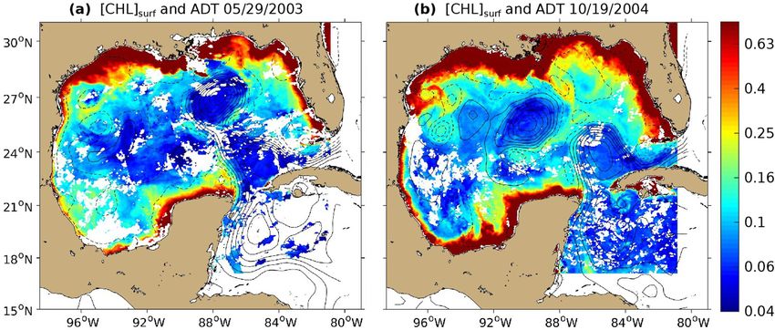
4282                                                                    P. Damien et al.: Productivity of Loop Current eddies

al., 2014; Mahadevan, 2014) and the ecosystem functioning         surface) [Chl] as a proxy for phytoplankton biomass and in-
(McGillicuddy et al., 1998, Oschlies and Garcon, 1998, Gar-       terpret a [Chl] increase as an effective biomass production.
con et al., 2001). Specifically, the ability of the mesoscale     Only a few studies considered the vertically integrated re-
eddies to enhance vertical fluxes of nutrients is a determi-      sponses (Dufois et al., 2017; Guo et al., 2017; Huang and Xu,
nant in sustaining the observed phytoplankton growth rate         2018) emphasizing the importance of considering the eddy
in oligotrophic regions such as the GoM open waters, where        impact on the subsurface.
the phytoplankton primary production is limited by nutrient          The objective of this study is to better understand the role
availability in the euphotic layer (McGillicuddy and Robin-       of LCEs in driving [Chl] distribution and variability within
son 1997; McGillicuddy et al., 1998; Oschlies and Garcon,         the GoM open waters. Material and methods used in this
1998).                                                            study are presented in Sect. 2. In Sect. 3, the imprint of
   The upward doming of isopycnals in cyclonic eddies and         the LCEs on the surface [Chl] distribution is inferred from
downward depressions in anticyclonic eddies, also known           satellite ocean color observations. Since these measurements
as “eddy pumping”, occur when the eddies are strength-            are confined to the oceanic surface layer and do not allow
ening (Siegel et al., 1999; Klein and Lapeyre, 2009) and          access to the vertical properties of LCEs, we complete the
produce a vertical nutrient transport. This has been histori-     analysis with a coupled physical–biogeochemical simulation
cally proposed as the dominant mechanism controlling the          (Sects. 2 and 3). Particular attention is paid to the valida-
mesoscale biogeochemical variability as it induces a reduc-       tion of the modeled LCE dynamical structures and surface
tion in productivity in the anticyclone and an increase in        [Chl] anomalies. In the last section, we propose to disentan-
cyclones. This paradigm is however challenged by observa-         gle the mesoscale mechanisms controlling the seasonal cycle
tions of enhanced surface chlorophyll concentrations in anti-     of the [Chl] vertical profile in LCEs. The model also enables
cyclonic eddies (Gaube et al., 2014), particularly during win-    us to assess both abiotic and biotic processes and physical–
ter (Dufois et al., 2016). As a plausible explanation, eddy–      biogeochemical interactions that can be difficult to address
wind interactions may significantly modulate vertical fluxes      with in situ observations only.
through Ekman transport divergence within the eddies (Mar-
tin and Richards, 2001; Gaube et al., 2013, 2015). This mech-
anism is responsible for a downwelling in the core of cy-         2     Material and methods
clones and an upwelling in the core of anticyclones. Dufois
et al. (2014, 2016) link these observations to a deeper mixed     2.1    The coupled physical–biogeochemical model
layer in anticyclonic eddies. This is explained by the eddy-
driven modulation of the upper ocean stratification which di-     The simulation analyzed in this study (referred to as
rectly affects the winter convective mixing (He et al., 2017).    GOLFO12-PISCES) has been described and compared with
Observed mixed layers tend to be deeper in anticyclones than      observations in Damien et al. (2018). It relies on a physical–
in cyclones (Williams, 1998; Kouketsu et al., 2012), and ver-     biogeochemical coupled model based on the ocean model
tical nutrient fluxes to the euphotic layer are potentially en-   NEMO (Nucleus for European Modeling of the Ocean,
hanced in anticyclones during periods prone to convection         version 3.6; Madec, 2016) and the biogeochemical model
(e.g., winter in the GoM). Although some consensus exists         PISCES (Pelagic Interaction Scheme for Carbon and Ecosys-
on the fundamental role of anticyclonic eddies on the produc-     tem Studies; Aumont and Bopp, 2006; Aumont et al., 2015).
tivity of oligotrophic ocean regions, large uncertainties re-     The model grid covers the GoM and the western part of
main regarding the relative importance of the different mech-     the Cayman Sea (Fig. 1) with a 1/12◦ horizontal resolution
anisms involved in the biogeochemical responses.                  (∼ 8.4 km). This allows us to resolve scales related to the
   In addition, in situ measurements in oligotrophic regions      first baroclinic mode, which is of the order of 30–40 km in
have shown that the surface [Chl] variability, observed from      the GoM open waters (e.g., Chelton et al., 1998). The model
ocean color satellite imagery, is not necessarily representa-     is forced with realistic open-boundary conditions from the
tive of the total phytoplankton (carbon) biomass variability      MERCATOR reanalysis GLORYS2V3, high-frequency at-
in the water column (Siegel et al., 2013; Mignot et al., 2014).   mospheric forcing based on an ECMWF ERA-Interim re-
In particular, a surface [Chl] winter increase may result from    analysis (Brodeau et al., 2010), and freshwater and nutrient-
physiological mechanisms (i.e., modification of the ratio of      rich discharges from rivers (Dai and Trenberth, 2002). The
[Chl] to phytoplankton carbon biomass) or from a vertical re-     open-boundary conditions of biogeochemical tracers are pre-
distribution of the phytoplankton (Mayot et al., 2017) rather     scribed from the World Ocean Atlas observation database
than from changes in the biomass content. It is not clear yet     (Garcia et al., 2010) for NO3 , O2 , Si, and PO4 and from
which of these hypotheses holds in oligotrophic regions and       the global configuration ORCA2 (Aumont and Bopp, 2006)
more specifically in the GoM open waters where this issue         for dissolved inorganic carbon (DIC), dissolved organic car-
has been addressed by in situ subsurface [Chl] observations       bon (DOC), Alkalinity, and Fe. The other state variables are
(Pasqueron de Fommervault et al., 2017). Most of the stud-        forced with very small constant values. The analysis has
ies focusing on chlorophyll variability use surface (or near-     been performed using 5 d averaged outputs for a period of

Biogeosciences, 18, 4281–4303, 2021                                                  https://doi.org/10.5194/bg-18-4281-2021
P. Damien et al.: Productivity of Loop Current eddies                                                                        4283

5 years from 2002 to 2007. We refer the reader to Damien           (Lipphardt et al., 2008; Hamilton et al., 2018) as LCE de-
et al. (2018) for extended model and numerical setup de-           struction and formation involves specific processes (Frolov
scriptions. In this previous study, an extensive validation of     et al., 2004; Donohue et al., 2016). We therefore focus on the
the modeled properties were carried out, focusing on phys-         LCEs contained in the central part of the GoM from 86 to
ical properties that are known to influence primary produc-        94◦ W. Annual composites are computed along with monthly
tion and chlorophyll concentration: the mixed layer depth          composite averages in order to assess seasonal variability.
and the depth and slope of the nutricline. A novel aspect was      Composite LCEs averaged during the months of January and
to use in situ observations collected from autonomous floats       February are referred to as winter composites, and those aver-
and published in Green et al. (2014) and Pasqueron de Fom-         aged during July and August are referred to as summer com-
mervault et al. (2017) to validate not only the modeled sur-       posites. These composites provide an overview of the LCEs
face chlorophyll concentration but also the chlorophyll verti-     mean hydrographical, biogeochemical, and dynamical char-
cal profile in the GoM. Starting from the parameters suitable      acteristics.
for global simulations (Aumont et al., 2015), a large tuning
of the biogeochemical model was carried out to reproduce           2.2.2   Diagnostics
the vertical profile of chlorophyll correctly. The ability of
GOLFO12-PISCES to reproduce the main observed features             The LCE radius RLCE is estimated as the radial distance
of the GoM was demonstrated, at least at a basin and seasonal      between the center and the peak azimuthal velocity Vmax .
scale.                                                             The mixed layer depth (MLD), a major physical factor influ-
                                                                   encing nutrient distribution and [Chl] dynamics (Mann and
2.2     Observational data set used                                Lazier, 2006), is defined as the depth at which potential den-
                                                                   sity exceeds its value at 10 m depth by 0.125 kg m−3 (Levi-
Satellite observations are used to evaluate the ability of         tus, 1982; Monterey and Levitus, 1997).
GOLFO12-PISCES to reproduce the dynamical and biolog-                 The stratification of the water column is evaluated by the
ical signatures associated with LCEs. Surface geostrophic          square of the buoyancy frequency N 2 (z) = −g       ∂ρ
                                                                                                                   ρ0 ∂z , where g
velocities are derived from a 1/4◦ multi-satellite merged          is the gravitational acceleration, z is depth, ρ is density, and
product of absolute dynamic topography (ADT) pro-                  ρ0 is a reference density.
vided by AVISO+ (http://marine.copernicus.eu, last access:            As carried out in Damien et al. (2018), several metrics are
10 April 2021). Surface chlorophyll concentrations are from        defined and used to describe [Chl]:
the Aqua-MODIS 4 km product (Sathyendranath et al., 2012;            – [Chl]surf is [Chl] averaged between 0 and 30 m
http://marine.copernicus.eu, last access: 10 April 2021) and           depth and considered as surface concentration (in
consist of 8 d composites from 2003 to 2015.                           mg Chl m−3 ).

2.2.1    LCEs detection, tracking, and composite                     – [Chl]tot is the integrated content of [Chl] over the 0–
         construction                                                  350 m layer (in mg Chl m−2 ).

In order to track the LCEs, we use the algorithm developed           – DCM is the depth of the deep chlorophyll maximum (in
by Nencioli et al. (2010), which has been extensively em-              m).
ployed to track coherent mesoscale eddies (Dong et al., 2012;        – [Chl]DCM is the [Chl] value at DCM depth (in
Ciani et al., 2017; Zhao et al., 2018) and submesoscale eddies         mg Chl m−3 ).
(Damien et al., 2017). It is based on the geometric organiza-
tion of the velocity fields, dominated by rotation, that develop   To understand the mesoscale distribution of [Chl], key bi-
around eddy centers. Here, it is applied to weekly AVISO+          ological variables are vertically integrated between 0 and
surface geostrophic velocities and GOLFO12-PISCES 5 d              350 m: the phytoplanktonic concentration [Phy]tot , the pri-
averaged velocities at 20 m depth. The selection of LCEs is        mary production rate PPtot , and the grazing rate GRZtot . PPtot
defined using the criteria that eddies have to be shed from the    consists of two components: new production PPNtot fueled
Loop Current.                                                      by nutrients supplied from a source external to the mixed
   In order to assess the [Chl] response to LCE dynamics,          layer and regenerated production PPRtot sustained by recy-
eddy-centric horizontal images and transects of LCEs are           cled nutrients within the euphotic layer (Dugdale and Goer-
used to make composites constructed by averaging mod-              ing, 1967; Eppley and Peterson, 1979). The euphotic depth
eled variables of the different LCEs collocated to their cen-      corresponds to 1 % of the incoming photosynthetic active ra-
ter. The transect building procedure involves an axisymmet-        diation at surface and reaches between 120 and 150 m in the
ric averaging that assumes axis symmetry of the dynamical          GoM (Jolliff et al., 2008; Linacre et al., 2019). A chloro-
structures and no tilting of their rotation axis. Moreover, we     phyll concentration anomaly within LCEs, [Chl]0 , is com-
choose not to consider the LCEs formation period and the           puted as [Chl]0 = [Chl] − [Chl], where [Chl] is the averaged
LCEs destruction period when reaching the western basin            background [Chl] field in the open GoM waters (for radius

https://doi.org/10.5194/bg-18-4281-2021                                                   Biogeosciences, 18, 4281–4303, 2021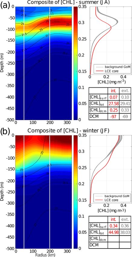
4284 P. Damien et al.: Productivity of Loop Current eddies
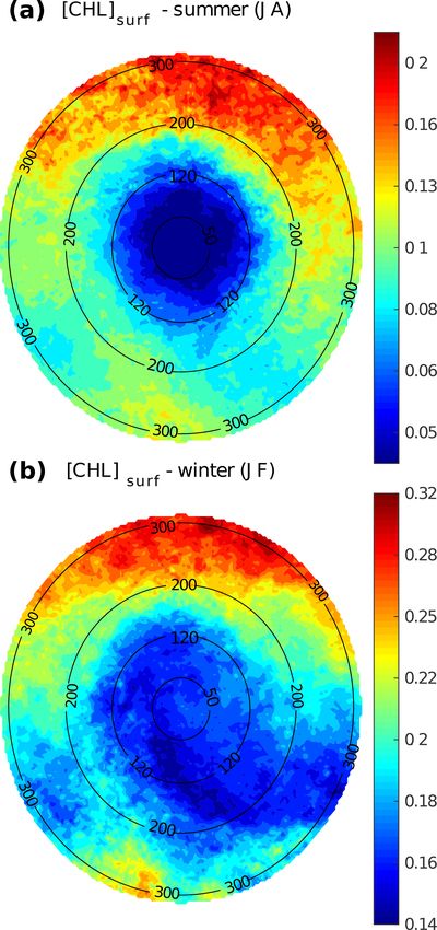
Figure 1. The 8 d composite images of [Chl]surf (in mg m−3 ) around (a) 29 May 2003 and (b) 19 October 2004 derived from Aqua-MODIS
images overlaid with contours of absolute dynamic topography (ADT; in m) derived from Aviso images are superimposed. Contour interval
is 10 cm, and ADT values lower than 40 cm are shown with dashed curves.
> 250 km from the LCEs’ centers). We also define the nor- the GoM open waters (Sheinbaum et al., 2016; Sturges and
malized anomaly as [Chl]0 /SD[Chl]0 , with SD the standard Leben, 2000; Hamilton, 2007; Jouanno et al., 2016).
deviation operator, following a similar approach as Gaube et LCE annual composites of surface geostrophic velocities
al. (2013, 2014) and Dufois et al. (2016). To limit the influ- (Fig. 2c) and [Chl]surf (Fig. 2d) are built from 482 differ-
ence of very high [Chl] values in coastal waters under the ent satellite images. On average, we found that RLCE is
direct influence of continental discharges, a salinity filtering ∼ 120 km and Vmax ∼ 0.6–0.7 m s−1 , in agreement with pre-
criterion (lower than 36 psu) is applied. A similar method viously reported LCEs (Elliot, 1982; Cooper et al., 1990;
was used by Gaube et al. (2013, 2014) to filter edge effects Forristal et al., 1992; Glenn and Ebbesmeyer, 1993; Weis-
but using a distance criterion instead. berg and Liu, 2017; Tenreiro et al., 2018). LCEs are asso-
ciated with a negative [Chl]surf anomaly (∼ −0.07 mg m−3
in the annual average). The LCEs’ influence on [Chl]surf is
3 Results largest in summer (Fig. 3a) when it reaches very low val-
ues (< 0.045 mg m−3 ), which correspond to an anomaly of
3.1 Satellite observations of [Chl] ∼ −0.08 mg m−3 . This anomaly is less remarkable in winter
(∼ −0.06 mg m−3 ; Fig. 3b) when [Chl]surf is ∼ 0.17 mg m−3
Figure 1 shows the 8 d averaged satellite observations of within LCEs. The high chlorophyll concentrations in the
the surface chlorophyll around 29 May 2003 (panel a) and northern part of the composites (in the southern part too but
19 October 2004 (panel b). These observations highlight in smaller proportions) are related to shelves.
the strong contrast between the eutrophic conditions in the
3.2 Dynamical characterization of modeled LCEs
coastal waters and the oligotrophic conditions in the open
ocean, as already addressed by several studies (Martinez- A total of 11 model LCEs were detected during the 5 years
Lopez and Zavala-Hidalgo, 2009; Pasqueron de Fommer- of simulation. Their trajectories are reported in Fig. 2b, su-
vault et al., 2017). Far from the coast, these figures also reveal perimposed upon the climatological EKE field simulated at
that the surface chlorophyll varies at a scale of the order of 10 m. The westward–southwestward propagation of LCEs
100 km with a distribution that tends to follow the absolute is well reproduced (Vukovich, 2007) even though the LCE
dynamic topography (ADT) contours. translation is almost westward in GOLFO12-PISCES. A
LCE trajectories are reported in Fig. 2a, superimposed comparison with Fig. 2a shows the ability of GOLFO12-
onto the geostrophic climatological eddy kinetic energy PISCES to represent the mean and transient dynamical fea-
(EKE) field at the surface. EKE is computed from eddy ve- tures of the GoM open waters (also see Garcia-Jove et al.,
locities defined on each grid cell as the difference between 2016).
the total horizontal current and its mean value over 120 d. The robustness of the composite method arises from the
This time window is chosen to filter the seasonal signal. EKE number of LCEs used to build the composites:
is concentrated in the Loop Current (LC) and on the west-
ward pathway of the LCEs (Lipphardt et al., 2008) demon- – Annual composite is built from 605 5 d averaged LCE
strating that LCEs constitute the major source of EKE in model outputs from 10 different LCEs.
Biogeosciences, 18, 4281–4303, 2021 https://doi.org/10.5194/bg-18-4281-2021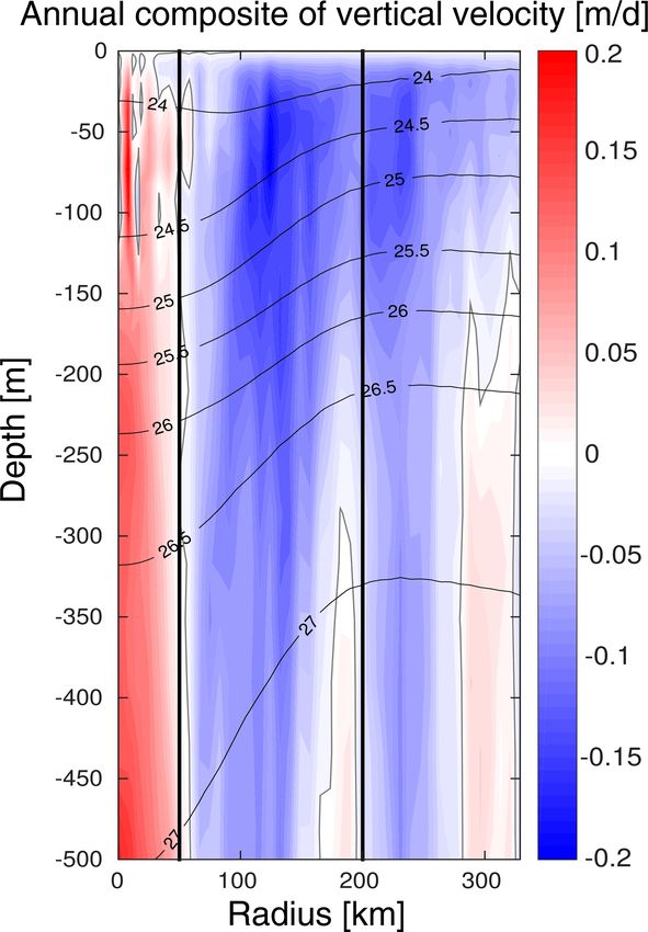
P. Damien et al.: Productivity of Loop Current eddies                                                                               4285

Figure 2. Average eddy kinetic energy (EKE) field derived from (a) Aviso geostrophic surface velocities and from (b) GOLFO12-PISCES
currents at 10 m depth. The trajectories of the tracked LCEs are superimposed to the EKE field (black lines). Dashed vertical black lines
indicate the central GoM area over which composites are built. Annual LCE composite images of surface geostrophic velocities for (c) Aviso
images and (e) GOLFO12-PISCES. Annual LCE composite images of surface chlorophyll concentration anomaly for (d) MODIS images,
and (f) GOLFO12-PISCES. Black circles indicate the radius in kilometers.

                                                                          – Summer composite is built from 83 5 d averaged LCE
                                                                            model outputs from 8 different LCEs.
                                                                          – Winter composite is built from 93 5 d averaged LCE
                                                                            model outputs from 9 different LCEs.
                                                                       The model LCE surface geostrophic velocities (Fig. 2e) have
                                                                       important similarities with velocities inferred from altimetry
                                                                       (Fig. 2c), confirming that GOLFO12-PISCES reproduces the
                                                                       surface signature of the LCEs. However, one can also notice
                                                                       an underestimation of the surface orbital velocities (∼ 25 %
                                                                       on average over the 50–200 km radius range). This bias could
                                                                       result from the relatively coarse model resolution and 5 d out-
                                                                       put frequency that are unable to fully capture the gradient in-
                                                                       tensity at RLCE . The assumption of an axial symmetry of the
                                                                       LCE circulation around its center also induces an error that
                                                                       tends to decrease Vmax .
                                                                          Orbital velocities of composite eddies are used to distin-
                                                                       guish different dynamical areas within LCEs. The model an-
                                                                       nual average dynamical profile at 25 m depth (Fig. 4) re-
                                                                       veals a typical vortex-like structure with RLCE ∼ 107 km and
                                                                       Vmax ∼ 0.53 m s−1 and suggests the following decomposi-
                                                                       tion:
                                                                          – r < 50 km is the LCE core where the eddy is approx-
                                                                            imately in solid body rotation: Vorb = a · r, where the
                                                                            coefficient a is related to the Rossby number (Ro =
                                                                            2a/f ). The ratio a/f is estimated to be ∼ −0.12
Figure 3. LCE composite images of [Chl]surf derived from Aqua-              (Fig. 4). In this field, the strain is reduced to a minimum
MODIS for the (a) summer and (b) winter seasons. Black circles              and the flow is dominated by rotation.
indicate the radius in kilometers.
                                                                          – 50 km < r < 200 km is the LCE ring structure where
                                                                            the orbital velocity reaches its maximum at RLCE and

https://doi.org/10.5194/bg-18-4281-2021                                                         Biogeosciences, 18, 4281–4303, 2021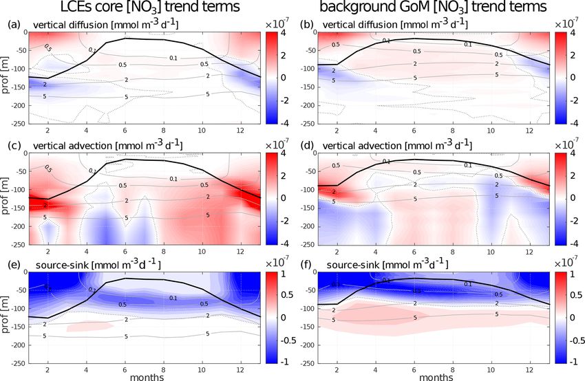
4286                                                                         P. Damien et al.: Productivity of Loop Current eddies

Figure 4. (a) Orbital velocities at 25 m depth as a function of the radius of each detected LCE (light gray dots). The red line is the LCE
orbital velocity profile of the annually averaged composite. (b) Vertical vorticity and strain
                                                                                              computed
                                                                                                       from the averaged orbital velocity
profile assuming no radial velocity in cylindrical coordinates as ζz = f1r ∂rv
                                                                           ∂r  and S = 1 ∂v − v .
                                                                                       f ∂r     r

     then decreases. The horizontal strain is important in this        characteristics close to the observed background GoM wa-
     field, even dominating vorticity from radius exceeding            ters (potential temperature ∼ 25.4 ◦ C and salinity ∼ 36.3 psu;
     RLCE .                                                            Meunier et al., 2018b) and is surrounded below and above by
                                                                       well-stratified layers (Meunier et al., 2018a). The upper py-
  – r > 200 km is the background GoM where the velocity
                                                                       cnocline varies seasonally and vanishes in winter due to the
    anomalies related to the LCEs vanish.
                                                                       deepening of the mixed layer, whereas the lower pycnocline
In the vertical (Fig. 5a), LCEs are near-surface intensified           is permanent.
anticyclonic vortex rings. At depth, the orbital peak veloc-              The downward displacement of isopycnals is accompanied
ity decreases rapidly. At 500 m depth, Vmax is ∼ 0.17 m s−1            by a depletion of nutrients in the upper layer of the LCE
and RLCE ∼ 75 km, and the dynamical LCE signal nearly                  core (Fig. 5e). This is a typical feature of mesoscale anti-
vanishes below 1500 m depth (Vmax < 0.03 m s−1 ). The pro-             cyclones in the ocean (McGillicuddy et al., 1998; Oschlies
posed division into three distinct dynamical regions applies           and Garcon, 1998). The 1 mmol m−3 iso-nitrate concentra-
from the surface down to 500 m depth (Fig. 5a).                        tion (hereafter ZNO3 , sometimes referred to as the nitracline
   The composite hydrological structure of modeled LCEs is             as in Cullen and Eppley, 1981, Pasqueron de Fommervault et
shown in Fig. 5b and c. The depression of isopycnals, asso-            al., 2017, and Damien et al., 2018) is located at ∼ 70 m depth
ciated with a depression of isotherms and isohalines, is char-         in the background GoM waters, whereas it is found much
acteristic of oceanic anticyclones. In the core of the eddies,         deeper in the core (ZNO3 ∼ 106 m). At depth, iso-nitrate lay-
the composite depicts a salinity maximum located between               ers and isopycnals are well correlated (Ascani et al., 2013;
100 and 300 m, corresponding to the signature of the At-               Omand and Mahadevan, 2015). For instance, iso-nitrate con-
lantic Subtropical Underwater (ASTUW) of Caribbean ori-                centration of 15 mmol m−3 follows the displacements of the
gin entering the GoM through the Yucatán Channel (Badan                1026.5 kg m−3 isopycnal. However, above 150 m, the den-
et al., 2005; Hernandez-Guerra and Joyce, 2000; Wuust,                 sity/nitrate relation is different inside and outside the ed-
1964). This salinity maximum is not limited to the core of             dies (ZNO3 is collocated with isopycnal 1024.4 kg m−3 in
the LCE but gradually erodes and shallows: 36.82 psu at                the LCE core and with isopycnal 1024.9 kg m−3 in the back-
200 m in the LCE core and 36.61 psu at 150 m in the back-              ground GoM).
ground GoM common water. Details on the fate of this salin-
ity maximum investigated with GOLFO12 simulations can                  3.3    Surface and vertical distribution of chlorophyll in
be found in Sosa-Gutiérrez et al. (2020). The ASTUW layer                     LCEs
(salinity > 36.5 psu) is also thicker in the LCE core (∼ 190 m
thick) compared to the background GoM water (∼ 120 m                   The large difference in stratification between the LCE core
thick). Overall, GOLFO12-PISCES reproduces the observed                and background GoM suggests a contrasted seasonal re-
hydrological structure of LCEs (Elliott, 1982; LeHenaff et             sponse of the [Chl]. This is evidenced by the analysis of sum-
al., 2012; Hamilton et al., 2018; Meunier et al., 2018b).              mer and winter composites of [Chl] vertical distribution.
   The annually averaged LCE composite presents a lens-                   In summer (Fig. 6a), [Chl]surf is ∼ 30 % lower in
shaped structure exhibiting a ∼ 50 m thick layer of weakly             the LCE core (r < 50 km) than in the background GoM
stratified waters located between 50 and 100 m depth                   (200 km < r < 330 km). A pronounced DCM, characteristic
(Fig. 5d). This subsurface modal water presents hydrological           of oligotrophic environments, is deeper in the core (∼ 97 m)

Biogeosciences, 18, 4281–4303, 2021                                                        https://doi.org/10.5194/bg-18-4281-2021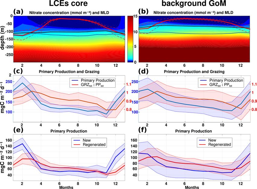
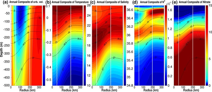
P. Damien et al.: Productivity of Loop Current eddies                                                                                 4287

Figure 5. Annually averaged LCE composite transects of (a) orbital velocities (m s−1 ), (b) potential temperature (◦ C), (c) salinity (psu),
(d) squared Brunt–Väisälä frequency (N 2 in s−2 ), and (e) nitrate concentration (mmol m−3 ). Isopycnal anomalies (black contours) are
superimposed on all panels. Vertical white lines delimit the three dynamical fields of the LCE composite. (e) Dashed red lines highlight two
specific iso-nitrate contours: 1 and 15 mmol m−3 .

than in the background GoM (∼ 69 m) with chlorophyll con-                  [Chl]tot is strongly shaped by both the seasonal variability
centrations significantly lower in the interior (∼ −25 %).              and the LCEs. The seasonal composites of [Chl]tot , shown in
   In winter, the [Chl] is maximum at the surface in all the            Fig. 7a, confirm the summer/winter contrast and highlight a
composite domains (Fig. 6b). [Chl]surf is lower in the LCE              monopole structure with a relatively homogeneous distribu-
core compared to the background GoM, but the difference                 tion of [Chl]tot within the eddy’s core. In order to better char-
is less marked (∼ −6 %) than in summer. The main discrep-               acterize the spatiotemporal variability in [Chl]tot induced by
ancy is the depth of the inflection point of these profiles. It is      LCEs, an empirical orthogonal function (EOF) analysis was
deeper in the LCE core (∼ −150 m), resulting in a more ho-              performed on the normalized [Chl]tot anomaly (Fig. 7b) fol-
mogenized [Chl] over a deeper layer than in the background              lowing the methodology of Dufois et al. (2016). It consists
GoM (∼ −120 m).                                                         of decomposing the signal into orthogonal modes of vari-
   However, despite reduced surface concentration both in               ability. Here, we choose to focus on the first two most sig-
winter and summer, the integrated chlorophyll content,                  nificant modes which explain 40.2 % and 9.9 % of the vari-
[Chl]tot , shows a distinct seasonal pattern compared to the            ability. Since they both depict a similar monopole structure
surface (Tables in Fig. 6).                                             in the LCE core, they were added up in a mode referred to
   In summer, [Chl]tot is lower in the LCE core                         as EOF 1 + 2 that is responsible for 50 % of the total [Chl]tot
(27.58 mg m−2 ) compared to the background GoM                          variance within LCEs. The third eigenmode (not shown) ac-
(29.41 mg m−2 ), and 1[Chl]tot = −1.83 mg m−2 .                         counts for 6.2 % and depicts a dipole structure with oppo-
   In winter, [Chl]tot is higher in the LCE core                        site polarity located at the east and north of the eddy center.
(44.98 mg m−2 ) compared to the background GoM                          On average, the EOF 1+2 mode is positive in winter (from
(38.03 mg m−2 ), and 1[Chl]tot = +6.95 mg m−2 .                         December to March) and negative the rest of the year (from
   The winter increase in [Chl]tot is around 29 % in the back-          April to November), with a maximum in December and Jan-
ground GoM, whereas it reaches 63 % in the LCE core, lead-              uary and a minimum in September. This justifies, a posteriori,
ing to [Chl]tot in the core being larger than [Chl]tot in the           the choice to consider winter and summer LCE composites.
background GoM in winter. Meanwhile, [Chl]surf remains                     The composite evolution of the LCE [Chl]tot along their
lower within the LCE core. The fact that the [Chl] at the               westward journey is shown in Fig. 8a and b. It illustrates how
surface does not reflect its depth-integrated behavior means            the total chlorophyll concentration is preferentially increased
that the peculiar variability in [Chl] within LCEs may not              in winter within the LCE core as soon as the LCEs are shed
be fully captured by ocean color satellite measurements.                from the LC. The winter [Chl]tot within LCEs is much larger
This is consistent with the observations and modeling results           (exceeding 1 standard deviation) than the background win-
of Pasqueron de Fommervault et al. (2017) and Damien et                 ter [Chl]tot . In terms of integrated [Chl], the LCE-induced
al. (2018) which addressed the vertical [Chl] distribution in           seasonal variability overwhelms the GoM open-water back-
the GoM.                                                                ground seasonal variability.

https://doi.org/10.5194/bg-18-4281-2021                                                          Biogeosciences, 18, 4281–4303, 2021
4288                                                                        P. Damien et al.: Productivity of Loop Current eddies

                                                                      Richards, 2001; Waite et al., 2007; Gaube et al., 2013; Du-
                                                                      fois et al., 2016, 2017; He et al., 2017), questioning the clas-
                                                                      sical paradigm of low productivity usually associated with
                                                                      anticyclonic eddies.
                                                                         The mechanisms explaining the LCE impact on [Chl] are
                                                                      discussed below, trying to rationalize the respective role of
                                                                      abiotic (e.g., trapping, winter mixing, Ekman pumping) and
                                                                      biotic processes (e.g., primary production, PP, grazing pres-
                                                                      sure, regenerated versus new PP).

                                                                      4.1    Eddy trapping

                                                                      The distinct hydrological and biogeochemical properties as-
                                                                      sociated with the LCE core suggest their ability to trap
                                                                      and transport oceanic properties. This mechanism, known as
                                                                      the eddy trapping (Early et al., 2011; Lehahn et al., 2011;
                                                                      McGillicuddy, 2015; Gaube et al., 2017), is efficient only if
                                                                      the orbital velocities of the vortex are faster than the eddy
                                                                      propagation speed (Flierl, 1981; d’Ovidio et al., 2013). The
                                                                      rotational velocities of the model LCEs are ∼ 0.53 m s−1
                                                                      and 1 order of magnitude larger than the propagation ve-
                                                                      locities (∼ 0.046 m s−1 on average). This suggests that LCEs
                                                                      might have a certain ability to trap the water masses present
                                                                      in their core with relatively low exchanges with the exterior.
                                                                         Salinity is well-suited to investigate water masses trapped
                                                                      within the LCE core during their propagation toward the
                                                                      western GoM (Fig. 8c; Sosa-Gutierez et al., 2020): salin-
                                                                      ity distribution shows a marked subsurface maximum that
                                                                      is not affected by biogeochemical processes. In the west-
                                                                      ern Caribbean Sea, ASTUW is characterized by high salin-
                                                                      ity (∼ 36.9 psu on average) and low standard deviation (<
                                                                      0.05 psu). The eastern GoM salinity field reveals that most
Figure 6. LCE composite transects of [Chl] during summer sea-         of the ASTUW crosses the Yucatán Channel within the Loop
son (a) and winter season (b). Density anomalies (black contours)     Current. During the formation of LCEs, a significant part of
are superimposed. Vertical white lines delimit the three dynami-      ASTUW is captured in the LCE core with low alteration of
cal fields of the LCE composite. For each season, [Chl] profiles in   its properties (Figs. 5c and 8c). Within the LCE core, the wa-
the LCE core (r < 50 km, red lines) and in the background GoM         ter mass is transported from the eastern to the western GoM
(200 km < r < 330 km, gray lines) are plotted. Key metrics con-       where its salinity decreases from 36.9 to 36.7 psu. Although
cerning [Chl] profiles are also indicated in the tables.              altered, the ASTUW signature is still clearly detectable in
                                                                      the GoM western boundary. The other part of ASTUW en-
                                                                      tering the GoM is found in the LCE ring. Compared to the
4   Discussion                                                        core, the salinity in the ring is on average lower (∼ 36.8 psu
                                                                      in the eastern GoM) and presents a high standard deviation,
In an oligotrophic environment such as the GoM open wa-               pointing out that more recent ASTUW co-exists with older
ters, the primary production is generally limited by nutrient         ASTUW that yields lower salinity maxima. As LCEs travel
supply, and [Chl]tot exhibits low seasonal variability at the         westward across the GoM, salinity in the LCE ring decays
GoM basin scale (Pasqueron de Fommervault et al., 2017).              rapidly to reach values similar to the background GoM val-
The winter increase in [Chl]tot within the LCE core (which            ues (∼ 36.6 psu). This homogenization mainly arises from
translates into an effective increase in biomass; see Ap-             vertical mixing and winter mixed layer convection (Sosa-
pendix A) contrasts with and may have large implications              Gutierez et al., 2020). Horizontal intrusions and filamenta-
for the regional biogeochemical cycles and ecosystem struc-           tion may also contribute to this homogenization (Meunier et
turation. It also echoes several studies which report elevated        al., 2020). The composites also suggest that almost no AS-
[Chl]surf within anticyclonic eddies in the oligotrophic sub-         TUW enters the GoM apart from the LCEs. The slight in-
tropical gyre of the southeastern Indian Ocean (Martin and            crease in the background salinity from the eastern to western

Biogeosciences, 18, 4281–4303, 2021                                                      https://doi.org/10.5194/bg-18-4281-2021
P. Damien et al.: Productivity of Loop Current eddies                                                                              4289

Figure 7. (a) Anomaly of [Chl]tot in summer and winter seasons. Black circles indicate the radius in kilometers. (b) EOF decomposition
of the normalized [Chl]tot anomaly. The spatial patterns and monthly magnitude (gray dots; the red line represents their monthly averaged
value) of the two first modes are indicated. Modes 1 and 2 were summed together and represent 50.1 % of the total variance.

                                                                       GoM is a consequence of the diffusion of salt from the LCEs
                                                                       toward the exterior.
                                                                          Although LCEs undergo considerable decaying rates, their
                                                                       erosion is particularly strong in the ring, while the core re-
                                                                       mains better isolated from the surrounding waters (Lehahn
                                                                       et al., 2011; Bracco et al., 2017). Since no significant [Chl]tot
                                                                       seasonal variability is reported in the western Caribbean Sea
                                                                       (Fig. 8), the biogeochemical behavior in the LCE core then
                                                                       has to be driven by local processes with the low influence
                                                                       of the horizontal advective process from the ring or of the
                                                                       Caribbean waters trapped during the LCE formation. Given
                                                                       that the LCE core is also quite homogeneous, the following
                                                                       discussion relies on the analysis of the seasonal cycles of se-
                                                                       lected parameters averaged within the LCE core.

                                                                       4.2   Nitracline depth and nutrient supply into the
                                                                             mixed layer

                                                                       The LCEs impact the upper ocean stratification (Fig. 5d), the
                                                                       nutricline depth (Fig. 5e), and consequently the nutrient sup-
                                                                       ply to the euphotic layer (McGillicuddy et al., 2015). The re-
                                                                       lationship between mixed layer deepening and nutrient sup-
                                                                       ply is studied here by comparing the ZNO3 with the MLD
                                                                       (Fig. 9a, b).
                                                                          In late-spring and summer (from May to September), the
Figure 8. (a) Summer [Chl]tot , (b) winter [Chl]tot , and (c) salin-
                                                                       water column is stratified (shallow MLD), and the downward
ity of Caribbean waters (ASTUW defined as the subsurface salinity
maximum) as a function of longitude in (red) the LCE core, in (blue)   displacement of the isopycnals within the LCEs pushes nu-
the LCE ring, and in (gray) the background GoM. Full lines indi-       trients below the euphotic zone (see also Figs. 5e, 6a): less
cate the averaged value and dashed lines the ± 1 standard deviation    nutrients are available within the LCE cores for phytoplank-
interval.                                                              ton growth, explaining a deeper and less intense DCM. In
                                                                       winter, the convective mixing, fostered both by intense buoy-
                                                                       ancy losses and strong mechanical energy input at the sur-

https://doi.org/10.5194/bg-18-4281-2021                                                        Biogeosciences, 18, 4281–4303, 2021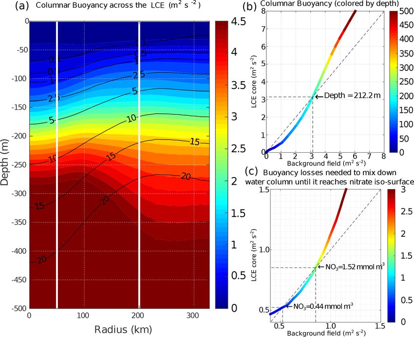
4290                                                                          P. Damien et al.: Productivity of Loop Current eddies

Figure 9. Climatological seasonal cycles of (a, b) nitrate concentration profiles (the red line overlaid is the average mixed layer depth, the
blue line is the base of the euphotic layer, and the black line is the nitracline), (c, d) the total primary production (blue) and the ratio of
grazing rate over primary production (red), and (e, f) the new (blue) and regenerated (red) primary production. Panels (a, c, e) refer to the
seasonal time series in the LCE core (r < 50 km), whereas the right panels (b, d, f) refer to the seasonal time series in the background GoM
(r > 200 km). For each average cycle, the mean value is shown (full line) along with its variability (±1 standard deviation relative to the
mean, dashed lines).

face, causes a larger deepening of the mixed layer within                 trient concentration levels in the LCE core compared to the
the LCE core (∼ −125 m; Fig. 9a) compared to the back-                    LCEs surrounding it. This likely explains the winter increase
ground (∼ −85 m; Fig. 9b). This asymmetry is due to a pro-                in surface nitrate concentration within the LCEs (Fig. 9a). In
nounced decrease in the surface and subsurface stratification             addition, a diagnostic of the different contributions to [NO3 ]
within the LCE core (Fig. 5d; see also Kouketsu et al., 2012).            evolution is proposed in Appendix B. It shows the dominant
A quantitative diagnosticR of the stratification is given by              role of vertical advection and diffusion in winter in providing
                           H
the columnar buoyancy, 0 N 2 (z) zdz, which measures the                  nutrients to the euphotic layer in the LCE core.
buoyancy loss required to mix the water column to a depth                    So far we have assumed that the surface buoyancy fluxes
H (Herrmann et al., 2008). Figure 10a reveals significant dif-            are identical over the LCE core and the background GoM.
ferences in pre-winter buoyancy between the eddy core and                 However, this is not strictly the case because temperature
its surroundings. Assuming that the change in buoyancy con-               and/or salinity features in the LCEs and background wa-
tent is mainly controlled by the buoyancy flux at the surface             ters are different (Fig. 5b, c; see also Williams, 1988). The
(see Turner, 1973; Lascaratos and Nittis, 1998), it suggests              modeled surface buoyancy loss during the winter season is
that mixing the water column down to ∼ −210 m depth re-                   ∼ 18 % more intense within the LCEs. This difference is
quires smaller surface buoyancy loss in LCE cores compared                substantial and probably mainly driven by additional surface
to the background GoM (Fig. 10b).                                         cooling applied to the warm LCE core through air–sea inter-
   However, the larger winter deepening of the mixed layer                action. It contributes to enhance convection within the eddy’s
within the LCE core is not a sufficient condition to explain a            core and then nutrient supply toward the surface.
larger nutrient supply. Indeed, it fosters the transport of nu-
trients from the nitracline toward the mixed layer because
both are getting closer. Figure 10c highlights that a smaller
buoyancy loss mixes down the water column to greater nu-

Biogeosciences, 18, 4281–4303, 2021                                                           https://doi.org/10.5194/bg-18-4281-2021
P. Damien et al.: Productivity of Loop Current eddies 4291
Figure 10. (a) Columnar buoyancy transect composite in summer, corresponding to pre-winter mixing season. Iso-nitrate concentrations
(black contours) are superimposed. Vertical white lines delimit the three dynamical fields of the LCE composite. (b) Vertical increase in the
columnar buoyancy in the LCE core versus the background GoM. Colors refer to depth. (c) Columnar buoyancy loss required to mix the
water column down to the iso-nitrate surface defined by the line color.
4.3 Productivity and grazing the PPRtot is dominant from April to October. During this
period, low NO3 resources are available in the euphotic
The primary productivity PPtot presents a clear seasonal cy- layer, and the ecosystem preferentially uses ammonium to
cle both in the LCE cores and in the background GoM with sustain the PPtot . This seasonal pattern is characteristic of
lower values in October–November, a sharp increase start- oligotrophic environments such as the GoM open waters
ing in November, a maximum in February, and a gradual de- (Wawrik et al., 2004; Linacre et al., 2015). In winter, changes
crease from March to October (Fig. 9c, d). The annual PPtot in PPtot are correlated with the intensity of winter mixing in
is slightly lower in the LCE core (∼ 142.4 mg C m−2 d−1 ) the LCE core (Fig. 9c) and the background GoM (Fig. 9d).
than in the background GoM (∼ 148.9 mg C m−2 d−1 ). The The larger PPNtot in the eddy core is consistent with a larger
amplitude of the seasonal cycle is larger in the LCE core: supply of [NO3 ] and is evidence that the core of anticyclones
from April to November, PPtot is on average ∼ 12 % lower can be preferential spots of enhanced biological production.
in the LCE core, whereas, in winter, PPtot is ∼ 14 % higher The pressure exerted by zooplankton grazers varies sea-
and reaches ∼ 243.2 mg C m−2 d−1 in February. Particularly sonally (Fig. 9c, d). It shows a similar seasonal cycle in the
in the LCE core, the PPtot seasonal cycle is tightly correlated LCE core and in the background GoM. On average, ∼ 90 %
with vertical mixing, revealing the important role of mixing of the total growth is consumed by grazers, reaching the high-
in the biogeochemistry. The relatively low standard devia- est impact in March, just one month after the peak season of
tion of the monthly PPtot distribution in the LCE core also the PPtot in both areas. In February the difference between
supports the idea that the influence of the seasonal variabil- the primary production and the grazing rate tends to be larger
ity in the forcing largely overwhelms their interannual and in the LCE core (GRZtot / PPtot = 0.95 ± 0.08) than in the
sub-monthly variability (Fig. 9c). GoM background (GRZtot / PPtot = 0.965 ± 0.13; Fig. 9c),
The ratio of the PPNtot and PPRtot provides informa- leading to an enhanced net primary production. Considering
tion about the mechanisms controlling the biomass growth the ecosystem from a “top-down” perspective, the grazing
(Fig. 9e, f). In winter, the PPNtot plays a leading role, reach- rate also participates then in enhancing [Chl]tot within the
ing up to 113–147 mg C m−2 d−1 , driven by the winter mix- LCE core compared to the background.
ing and induced [NO3 ] fluxes (see Appendix B). Conversely,
https://doi.org/10.5194/bg-18-4281-2021 Biogeosciences, 18, 4281–4303, 20214292 P. Damien et al.: Productivity of Loop Current eddies
4.4 Eddy–wind interactions
In summer, the total primary production is higher in the back-
ground GoM waters as the regenerated production rate is
higher. Since grazing is known to be a major contributor
of the recycling loop in the euphotic zone (Sherr and Sherr,
2002), the lower grazing rate inside the LCE during summer
(Fig. 9c, d) likely explains this lower regenerated production.
In addition, the biogeochemical consumption of nitrate that
fosters the production of organic matter occurs in a deeper
layer within the LCE core compared to the background GoM
(Fig. B1e, f). It is then more likely exported out of the eu-
photic layer in the form of a settling particle, leading to lower
remineralization rates in the upper layers to feed regenerated
production. More surprising, the new primary production ex-
hibits similar rates in both regions, although NO3 depletion
occurs deeper in the LCE core. In the absence of a strong
enough vertical mixing when the mixed layer is shallow, this
apparent mismatch requires an additional mechanism, verti-
cal advection, capable of supplying NO3 to the euphotic layer
(Sweeney et al., 2003; McGillicuddy et al., 2015). Figure 11. Annually averaged LCE composite transects of verti-
The model vertical velocity in the LCEs reveals an up- cal velocities (m d−1 ). Isopycnals anomalies (black contours) are
superimposed on all panels. Vertical white lines delimit the three
ward pumping in their core (Fig. 11). The vertical veloc-
dynamical fields of the LCE composite.
ity between 100 and 500 m is on average + 0.07 m d−1 . This
vertical transport is mainly driven by two mechanisms, eddy
pumping (Falkowski et al., 1991) and eddy–wind interaction
(Dewar and Flierl, 1987), but their relative importance is dif- ward pumping in the eddy interior (see Martin and Richards,
ficult to quantify (Gaube et al., 2014; McGillicuddy et al., 2001; Gaube et al., 2013, 2014, for further details). With
2015). ρ0 ∼ 1023 kg m−3 and f ∼ 6.2 × 10⁻⁵ s−1 , we estimate WE
The eddy pumping mechanism is related to the decay of to range from + 0.06 to 0.13 m d−1 , in agreement with the
the rotational velocities from the moment LCEs are released modeled vertical velocity within the core. The eddy-Ekman
from the Loop Current. In the LCE core, this decay is con- pumping mechanism could explain a large fraction of the
sidered as moderate since lateral diffusivity is expected to gradual upwelling within the eddy’s core (Fig. 11) and may
be relatively low (Sect. 4.1). This process may however be actively contribute to the advective vertical flux of nutrients
considerable in the LCE ring where the erosion rates are im- (see Appendix B). In summer, this mechanism could explain
portant (Meunier at al., 2020). why new primary production rates are similar in the LCE
Eddy–wind interactions are due to mesoscale modulation core and the background GoM waters, although the nutrient
of the Ekman transport so that they are often qualified as pool is located much deeper in the LCE core.
eddy-Ekman pumping (He et al, 2017). Following the ob- The eddy-Ekman pumping persists in the LCE core
servation of an LCE core in quasi-solid body rotation, the throughout its lifetime as long as there is a wind stress ap-
horizontal vorticity varies little with the radius resulting in a plied at the surface. During wintertime, we expect that both
negligible “non-linear” contribution of the Ekman pumping vertical mixing and eddy-Ekman pumping participate to in-
(McGillicuddy et al., 2008; Gaube et al., 2015). Assuming a crease the new primary production. A question then arises
small effect of the eddy SST-induced (sea surface tempera- about the relative contribution of winter mixing to eddy-
ture) Ekman pumping, the total Ekman pumping simplifies Ekman pumping in the LCE core primary production in-
into its “linear” contribution, computed as WE = ρ0∇×τ (f +ζ ) , crease in winter. This issue was tackled by He et al. (2017)
where ρ0 is the surface density, f the Coriolis parameter, τ and Travis et al. (2020) comparing the rate of change in the
the stress at the sea surface depending on both the wind and mixed layer depth with the vertical velocity induced by the
ocean currents at the surface (Martin and Richards, 2001, eddy-Ekman pumping (Eq. 4 in He et al, 2017). In the GoM,
their Eq. 12), and ∇× the curl operator. Considering uni- even if the wind shows larger magnitudes in winter, it is
form wind velocities ranging from 4.5 to 7.5 m s−1 (Nowlin also associated with a large variability. As a consequence,
and Parker, 1974; Passalacqua et al., 2016) blowing over the the variability in Ekman pumping is also found to be large,
LCE, the curl of the stress arises from the anticyclonic sur- and a robust seasonal cycle which would allow us to isolate
face circulation generated by the eddy. Its manifestation is a the Ekman pumping in winter cannot be clearly identified.
persistent horizontal divergence at surface balanced by an up- However, in the LCE core, we estimate the mixed layer to
Biogeosciences, 18, 4281–4303, 2021 https://doi.org/10.5194/bg-18-4281-2021P. Damien et al.: Productivity of Loop Current eddies 4293
deepen at roughly 0.8 m d−1 , which is on average about 1 The under-representation of these profiles, potentially due to
order of magnitude larger than the higher bound of the esti- a relatively coarse model resolution, could be associated with
mated pumping mechanism typically occurring in winter in an underestimation of [Chl]tot in winter. The results exposed
response to stronger wind events. This supports winter mix- in this study would require further confirmation, notably by
ing as the overwhelming process for the LCE-induced pri- more subsurface in situ measurements, in particular within
mary production peak in winter. the core of LCEs where no [Chl] profiles were observed in
winter.
Although the biological response to LCEs may present
5 Summary and perspectives some specificities due to the particular dynamical nature of
LCEs, this study suggests potentially generic insights on the
The [Chl] variability induced by the mesoscale Loop Cur- biogeochemical role that anticyclonic eddies could play in
rent eddies in the Gulf of Mexico is studied by analyzing oligotrophic environments. It echoes the previous works of
vortex composite fields generated from a coupled physical– Martin and Richards (2001), Gaube et al. (2014, 2015), and
biogeochemical model at 1/12◦ horizontal resolution. LCEs especially Dufois et al. (2014, 2016) and He et al. (2017)
are hotspots for mesoscale biogeochemical variability. De- who proposed winter vertical mixing as an explanation for
spite the [Chl]surf negative anomaly associated with their the positive [Chl]surf anomaly observed in anticyclones in the
core (r < 50 km), model results indicate that LCEs are as- southern Indian Ocean. One of the most crucial points to be
sociated with enhanced phytoplankton biomass content, par- underlined from our results is that the enhanced primary pro-
ticularly in winter. This enhancement results from the contri- duction and biomass content within anticyclonic eddies may
bution of multiple mechanisms of physical–biogeochemical not necessarily be correlated with the surface layer variabil-
interactions and contrasts with the background oligotrophic ity. In oligotrophic areas, the integrated content of chloro-
surface waters of the GoM. phyll in the water column has to be considered. This implies
The main results of this study are the following: that caution should be exercised in the analysis and interpre-
– LCE cores present a negative surface chlorophyll tation of [Chl]surf observed by remote sensing instruments
anomaly. and highlights the crucial need for in situ biogeochemical and
bio-optical measurements. In oligotrophic environments, de-
– Unlike [Chl]surf , [Chl]tot is larger in the LCE cores com- fined by their low production rates and their low chlorophyll
pared to the background GoM in winter. concentration, anticyclonic eddies are able to trigger local
enhanced biological productivity and generate phytoplank-
– LCE cores trigger a large phytoplankton biomass in- ton biomass positive anomalies. In a scenario of expansion
crease in winter. of oligotrophic areas (Barnett et al., 2001; Behrenfeld et al.,
2006; Polovina et al., 2008), the fate and role of mesoscale
– The winter mixing is a key mesoscale mechanism that
anticyclones is an important aspect to be considered.
preferentially supplies nutrients to the euphotic layer
This study focuses on mesoscale physical–biogeochemical
within the LCE core. Consequently, it drives an eddy-
interactions, which is the spectral range resolved by the
induced peak of new primary production.
GOLFO12-PISCES configuration. It is evidence of the im-
– Eddy-Ekman pumping is a significant mechanism for portant role of mixing in primary production in the LCE core
sustaining relatively high new primary production rates at seasonal scale. However, mixing also presents significant
within LCE cores during summer. fluctuations at higher frequencies, associated with particular
atmospheric events like storms. The PPtot response to such
The phytoplankton biomass increase in individual LCE cores forcing requires further investigation to verify if the corre-
suggests that LCEs play an important role in sustaining the lation between PPtot and mixing still holds at higher fre-
large-scale GoM productivity. quencies where other additional drivers might also become
GOLFO12-PISCES provides numerical results which important. For instance, the role of submesoscale is of par-
largely conformed to observations. This extensive validation ticular interest since it has been proven to trigger mecha-
gives confidence about its ability to produce realistic sea- nisms of significant importance for biogeochemistry (Lévy
sonal and mesoscale variability in biogeochemical tracers at et al., 2018). Higher model resolutions can locally enhance
surface and subsurface, in particular the one associated with density gradients (Lévy et al., 2012; Omand et al., 2015)
LCEs. However, biases are inherent to the model and might leading to ageostrophic circulations that perturb the circu-
affect the main conclusions drawn. For example, in situ mea- lar flow around vortices (Martin and Richards, 2001) or en-
surements reveal an intense variability in [Chl] vertical pro- hanced vertical velocities that potentially foster the nutrient
files in winter that the model tends to underestimate (Green supply to the euphotic layer. Beside the mesoscale Ekman
et al., 2014; Damien et al., 2018). In particular, some in- pumping located at the eddy center, eddy–wind interactions
dividual observed profiles in winter present a DCM, while also produce vertical velocities at the eddy periphery (e.g.,
GOLFO12-PISCES largely favors well-mixed [Chl] profiles. Flierl and McGillicuddy, 2002). Finally, it is also worth not-
https://doi.org/10.5194/bg-18-4281-2021 Biogeosciences, 18, 4281–4303, 20214294 P. Damien et al.: Productivity of Loop Current eddies ing that anticyclonic mesoscale eddies are capable of trap- ping near-inertial energy waves in the ocean (Kunze, 1985; Danioux et al., 2008; Koszalka et al., 2010; Pallas-Sanz et al., 2016) where they produce vertical recirculation patterns (Zhong and Bracco, 2013). Even if some of these dynamical aspects are partially resolved at 1/12◦ horizontal resolution, higher resolutions simulations with higher frequency outputs are necessary to correctly assess their specific impact. Biogeosciences, 18, 4281–4303, 2021 https://doi.org/10.5194/bg-18-4281-2021
P. Damien et al.: Productivity of Loop Current eddies                                          4295

Appendix A: [Chl] / C-biomass ratio and ecosystem
structure

[Chl] is widely used as a proxy for photosynthetic biomass
(Strickland, 1965; Cullen, 1982). However, in addition to de-
pending on phytoplankton concentration, it is also affected
by several other factors mainly produced by intracellular
physiological mechanisms (Geider, 1987). In particular, pho-
toacclimation processes have been proven to be determinant
to explain [Chl]surf variability in oligotrophic areas (Mignot
et al., 2014). In the GoM open waters, this issue was specif-
ically addressed at a basin scale in Pasqueron de Fommer-
vault et al. (2017) considering in situ particulate backscat-
tering measurements and in Damien et al. (2018) from mod-
eling tools. They both reach the same conclusion: [Chl]tot
variability provides a reasonably good estimate of the total C
biomass variability ([Phy]tot ).
   This is confirmed by the small amplitude of the sea-
sonal cycle of the ratio [Chl]tot / [Phy]tot in the background
GoM (0.256 ± 0.004 g mol−1 averaged throughout the year;
Fig. A1). In the LCE core, this statement is still valid but
must be qualified since the ratio [Chl]tot / [Phy]tot presents
small but significant changes through the year (Fig. A1a).
It is around 0.24 g mol−1 from March to November and in-
creases sharply in December to reach about 0.32 g mol−1 in
January and February. As a result, in winter, the photoaccli-
mation mechanism accounts for ∼ 25 % of the total [Chl]tot
increase (the remaining part being an effective phytoplankton
biomass increase). In summer, the ratio [Chl]tot / [Phy]tot is
slightly lower in the LCE core compared to the background
GoM. As a consequence, the [Chl]tot negative anomaly asso-
ciated with the LCE core does not necessarily translate into
a [Phy]tot negative anomaly.
   Overall in the GoM open waters, there is a dominance
of the small-size phytoplankton over the large-size class in
proportions close to 80 % : 20 % (Linacre et al., 2015). Al-
though the modeled ecosystem structure is relatively sim-
ple, this typical community size structure is well reproduced
by GOLFO12-PISCES (Fig. A1c and d), which also sug-
gests a shift in the ecosystem structure in winter. The dif-
ferent response among size classes results from the enhance-
ment of nutrient vertical flux. The role of “secondary” nutri-
ents in this change in the community composition must also
not be overlooked, in particular for diatoms (accounted in
the model’s large-size group) since they also uptake silicate
(Benitez-Nelson et al., 2007). Moreover, GOLFO12-PISCES
exhibits a modulation of the ecosystem structure by LCEs.
The dominance of small-size phytoplankton is slightly more
marked in summer, and the winter shift is stronger in the LCE
core.

https://doi.org/10.5194/bg-18-4281-2021                          Biogeosciences, 18, 4281–4303, 2021
You can also read