Using phase lags to evaluate model biases in simulating the diurnal cycle of evapotranspiration: a case study in Luxembourg - HESS
←
→
Page content transcription
If your browser does not render page correctly, please read the page content below
Hydrol. Earth Syst. Sci., 23, 515–535, 2019
https://doi.org/10.5194/hess-23-515-2019
© Author(s) 2019. This work is distributed under
the Creative Commons Attribution 4.0 License.

Using phase lags to evaluate model biases in simulating the diurnal
cycle of evapotranspiration: a case study in Luxembourg
Maik Renner1 , Claire Brenner2 , Kaniska Mallick3 , Hans-Dieter Wizemann4 , Luigi Conte1 , Ivonne Trebs3 ,
Jianhui Wei4 , Volker Wulfmeyer4 , Karsten Schulz2 , and Axel Kleidon1
1 Max   Planck Institute for Biogeochemistry, 07745 Jena, Germany
2 Institut für Wasserwirtschaft, Hydrologie und konstruktiven Wasserbau,
Universität für Bodenkultur (BOKU), 1190 Vienna, Austria
3 Department of Environmental Research and Innovation, Luxembourg Institute of Science

and Technology (LIST), 4422 Belvaux, Grand Duchy of Luxembourg
4 Institut für Physik und Meteorologie, Universität Hohenheim, 70599 Stuttgart, Germany

Correspondence: Maik Renner (mrenner@bgc-jena.mpg.de)

Received: 4 June 2018 – Discussion started: 9 July 2018
Revised: 21 November 2018 – Accepted: 29 December 2018 – Published: 28 January 2019

Abstract. While modeling approaches of evapotranspira-           different mechanisms of diurnal heat storage and exchange
tion (λE) perform reasonably well when evaluated at daily        and, thus, allow a process-based insight to improve the repre-
or monthly timescales, they can show systematic deviations       sentation of land–atmosphere (L–A) interactions in models.
at the sub-daily timescale, which results in potential biases
in modeled λE to global climate change. Here we decom-
pose the diurnal variation of heat fluxes and meteorological
variables into their direct response to incoming solar radia-    1   Introduction
tion (Rsd ) and a phase shift to Rsd . We analyze data from an
eddy-covariance (EC) station at a temperate grassland site,      Evapotranspiration and the corresponding latent heat
which experienced a pronounced summer drought. We em-            flux (λE) couple the surface water and energy budgets and
ploy three structurally different modeling approaches of λE,     are of high relevance for water resources assessment. λE is
which are used in remote sensing retrievals, and quantify        generally limited by four physical factors: (i) the availability
how well these models represent the observed diurnal cy-         of energy mostly supplied by solar radiation, (ii) the avail-
cle under clear-sky conditions. We find that energy balance      ability of and the access to water, (iii) the plant physiology,
residual approaches, which use the surface-to-air tempera-       and (iv) the atmospheric transport of moisture away from the
ture gradient as input, are able to reproduce the reduction      surface (Brutsaert, 1982). These different limitations have
of the phase lag from wet to dry conditions. However, ap-        led to different approaches on how to model λE.
proaches which use the vapor pressure deficit (Da ) as the          Key approaches either focus on the surface energy bal-
driving gradient (Penman–Monteith) show significant devia-       ance where the surface-to-air temperature gradient dominates
tions from the observed phase lags, which is found to depend     the flux or approaches which focus on the moisture trans-
on the parameterization of surface conductance to water va-      fer limitation where vapor pressure gradients dominate the
por. This is due to the typically strong phase lag of 2–3 h      flux. It is critical to recognize that these two limitations are
of Da , while the observed phase lag of λE is only on the        not independent of each other but rather are shaped by land–
order of 15 min. In contrast, the temperature gradient shows     atmosphere heat and water exchange and thus covary with
phase differences in agreement with the sensible heat flux       each other. The diurnal variation of incoming solar radia-
and represents the wet–dry difference rather well. We con-       tion (Rsd ) causes a strong diurnal imbalance in surface heat-
clude that phase lags contain important information on the       ing leading to the pronounced diurnal cycles of surface states
                                                                 and fluxes (Oke, 1987; Kleidon and Renner, 2017). This

Published by Copernicus Publications on behalf of the European Geosciences Union.
516   M. Renner et al.: Using phase lags to evaluate model biases in simulating the diurnal cycle of evapotranspiration

heat exchange of the surface with the lower atmosphere thus        interest against the forcing variables and its first-order time
influences the near-surface air temperature (Ta ), skin tem-       derivative. This simple model allows estimating storage ef-
perature (Ts ), vapor pressure (ea ), soil or canopy saturation    fects on diurnal (Sun et al., 2013) to seasonal timescales
water pressure (es ), vapor pressure deficit (Da ), and wind       (Duan and Bastiaansen, 2017).
speed (u), which are being regarded as important controls             Here, we choose the Camuffo and Bernardi (1982) model
on λE (e.g., Penman, 1948). These interactions are particu-        because it provides an objective measure of the magnitude
larly dominant at the diurnal timescale (e.g., De Bruin and        of hysteresis loops and it allows for an assessment of statisti-
Holtslag, 1982) and depend on meteorological as well as on         cal significance. We extend the Camuffo and Bernardi (1982)
surface conditions (Jarvis and McNaughton, 1986; van Heer-         model in two ways.
waarden et al., 2010). Ignoring the interdependence of the            First, we use incoming solar radiation (Rsd ) as a refer-
surface variables may lead to biases in model parameteri-          ence variable instead of net radiation to estimate the phase
zations and compensating errors when evaluating the model          lag of surface heat flux observations and models. And sec-
performance only with respect to a single variable (Matheny        ondly, we use a harmonic transformation of the Camuffo and
et al., 2014; Best et al., 2015; Santanello et al., 2018).         Bernardi (1982) regression model to estimate the phase lag in
   There is a strong need to investigate and to derive metrics     time units. This extension allows us to compare the diurnal
based on comprehensive observations that characterize the          phase lag signatures of the different model inputs and how
whole land-surface–atmosphere system (Wulfmeyer et al.,            these influence the resulting diurnal course of the latent heat
2018). Several authors proposed different multivariate met-        flux estimate.
rics to better evaluate land–atmosphere (L–A) interactions            We specifically choose incoming solar radiation Rsd as the
in observations and models. Generally, these metrics explore       reference for the phase-shift analysis, since Rsd can be re-
internal relationships between state variables to better char-     garded as an independent forcing of the surface energy bal-
acterize key processes and to guide a more systematic ex-          ance (e.g., Ohmura, 2014):
ploration and understanding of model deficiencies. A num-
                                                                   Rsd (1 − α) + Rld − H − λE − G = σ T 4 + m,                  (1)
ber of metrics focus on the diurnal evolution of the heat and
moisture budgets in the planetary boundary layer (e.g., Betts,     with surface albedo α, incoming longwave radiation Rld , sen-
1992; Santanello et al., 2009, 2018). Also statistical metrics     sible heat flux H , latent heat flux λE, the conductive soil heat
exploring the strength of linear relationships between sur-        flux G, the outgoing longwave radiation σ T 4 , and storage
face heat fluxes and states to surface radiation components        terms of the surface layer summarized in m. This formula-
have been employed to evaluate the performance of reanal-          tion of the surface energy balance provides the direction of
ysis with observations (Zhou and Wang, 2016; Zhou et al.,          the energy exchange processes at the surface, illustrating that
2017, 2018).                                                       the terms on the right-hand side depend on heat fluxes on
   Furthermore, there are pattern-based metrics which focus        the left-hand side of Eq. (1) (Ohmura, 2014). As a conse-
on nonlinear interactions at the diurnal timescale. Wilson         quence, the term net radiation Rn , which resembles the ra-
et al. (2003) proposed the method of a diurnal centroid to         diation budget of the shortwave and longwave components,
measure the timing of the surface heat fluxes and their tim-       Rn = Rsd (1 − α) + Rld − σ T 4 , cannot be regarded as an in-
ing difference, which was more recently used by Nelson et          dependent surface forcing. Consequently, we choose Rsd in-
al. (2018) to quantify the timing of evapotranspiration un-        stead of Rn or Rn −G as the reference variable for the phase-
der different dryness condition for the FLUXNET dataset.           shift analysis of the latent heat flux and the main input vari-
In contrast, Matheny et al. (2014) and Zhang et al. (2014)         ables of evapotranspiration model approaches.
explored the diurnal relationship of the latent heat flux to va-      We focus on two different approaches to estimate λE.
por pressure deficit showing a pronounced hysteresis loop.         The first approach is based on the energy limitation of λE,
Zheng et al. (2014) also included air temperature and net ra-      using the equilibrium evaporation concept (Schmidt, 1915)
diation as reference variables and showed that the hystere-        as formulated by Priestley and Taylor (1972) for potential
sis loops of λE to Da or Ta are large, while there are only        evaporation. For actual evaporation we focus on one-source
small hysteresis effects when Rn was used. Hysteresis loops        and two-source energy balance schemes (OSEB and TSEB,
have also been found when heat fluxes are plotted against          respectively) which derive λE as the residual term of the
net radiation (Camuffo and Bernardi, 1982; Mallick et al.,         surface energy balance and parameterize the sensible heat
2015), with many studies showing hysteretic loops of the soil      flux by a resistance description of the surface-to-air tem-
heat flux against net radiation (Fuchs and Hadas, 1972; San-       perature gradient (Kustas and Norman, 1999). The second
tanello and Friedl, 2003; Sun et al., 2013). The presence of a     approach is based on the Penman–Monteith (PM hereafter)
hysteresis loop indicates that there is a time-dependent non-      approach (Monteith, 1965), which adds water vapor pres-
linear control on the variable of interest, typically induced by   sure deficit as a driving gradient (referred to as the “vapor-
heat storage processes. Camuffo and Bernardi (1982) showed         gradient scheme”). We use the widely used Food and Agri-
that the magnitude and direction of such hysteretic loops can      culture Organization of the United Nations (FAO) Penman–
be estimated by a multilinear regression of the variable of        Monteith formulation (Allen et al., 1998) for potential or

Hydrol. Earth Syst. Sci., 23, 515–535, 2019                                       www.hydrol-earth-syst-sci.net/23/515/2019/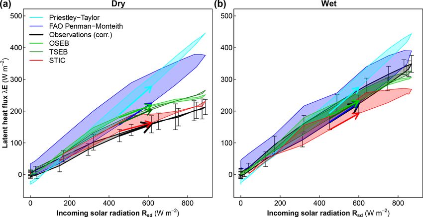
M. Renner et al.: Using phase lags to evaluate model biases in simulating the diurnal cycle of evapotranspiration                  517

reference evapotranspiration. For actual evapotranspiration
we use a modified PM approach which was formulated by
Mallick et al. (2014, 2015, 2016, 2018) (see also Bhattarai et
al., 2018) and is termed as a the Surface Temperature Initi-
ated Closure (STIC). STIC is based on finding the analytical
solution of the surface and aerodynamic conductances in the
PM equation while simultaneously constraining the surface
and aerodynamic conductances through both surface temper-
ature and vapor pressure deficit.
   Several inter-comparison studies evaluated the perfor-
mance of these schemes using observations from different
landscapes. OSEB and TSEB, which are often used in remote
sensing retrievals of λE, have been found to perform compa-
rably well in reproducing tower-based energy flux observa-
tions (Timmermans et al., 2007; Choi et al., 2009; French et
al., 2015). Yang et al. (2015) compared temperature-gradient
approaches (including TSEB) with the Penman–Monteith
approach (based on vapor pressure gradient only) employed
by the MODIS evapotranspiration product (MOD16, Mu et
al., 2011) and found strongly reduced capability of MOD16
to estimate spatial variability of evapotranspiration. They
concluded that the moisture availability information obtained
from the relative humidity and vapor pressure deficit of the
air is not able to capture the surface water limitations as re-
flected in surface temperature.
   In this study, we focus on the ability of these different
evapotranspiration models to reproduce the diurnal cycle
of λE under wet and dry conditions. In particular, we as-
sess if significant nonlinear relationships in the form of hys-
teretic loops exist, if these change under different wetness
                                                                  Figure 1. Illustration of a pattern-based evaluation of the diurnal
conditions, and if temperature-gradient and vapor-gradient
                                                                  cycle. (a) shows the diurnal cycle of Rsd under clear-sky condi-
approaches such as PM are able to reproduce this behavior.        tions and the diurnal cycle of two variables Y1 and Y2 , one in phase
Further, we evaluate which input variables of the evapotran-      with Rsd and another lagging Rsd . (b) illustrates the relationship of
spiration schemes show a hysteretic pattern and how these         these variables when plotted against Rsd . The bold arrow indicates
patterns influence the flux estimation. To address these ques-    the direction of the loop and the area inside the hysteresis describes
tions, we analyze observations and models with respect to         the magnitude of the phase shift.
internal functional relationships (pattern-based) and use so-
lar radiation as an independent driver of land–atmosphere
exchange. We focus on wet vs. dry conditions since this           teractions and, thus, guide process-based improvements and
is another critical deficiency identified in previous analyses    calibration of land-surface schemes.
(e.g., Wilson et al., 2003; Matheny et al., 2014; Zhou and
Wang, 2016). To ensure similar radiative forcing and avoid
variability due to cloud cover we focus the evaluation on         2     Methods and data
clear-sky days. We illustrate our approach on a grassland
site in a temperate semi-oceanic climate using surface energy     2.1    Diurnal patterns and hysteresis loop quantification
balance observations.
   The analysis will shed light on the capabilities of process-   We first illustrate the pattern-based evaluation of the diurnal
based evapotranspiration schemes to capture the dynamics of       cycle using two hypothetical variables Y1 and Y2 , as shown
diurnal land–atmosphere exchange. We show that the phase          in Fig. 1. If a variable (Y1 ) is in phase with Rsd , it shows
lag of surface states and fluxes reveals important imprints of    a linear behavior when plotted against Rsd (Fig. 1b). How-
heat storage processes and how this guides the evaluation of      ever, if a variable (Y2 ) has a time lag with respect to Rsd ,
the different approaches for modeling λE. This is important       showing a significant difference between morning and after-
for applications in remote sensing with respect to the choice     noon values, it results in a hysteretic loop. The area inside the
of observational input variables. In doing so, we provide a       loop indicates the magnitude of the phase difference, while
further, pattern-based metric to assess land–atmosphere in-       the direction of the loop, marked by an arrow at the morning

www.hydrol-earth-syst-sci.net/23/515/2019/                                         Hydrol. Earth Syst. Sci., 23, 515–535, 2019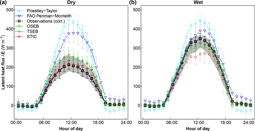
518    M. Renner et al.: Using phase lags to evaluate model biases in simulating the diurnal cycle of evapotranspiration

rising limb in Fig. 1b, indicates if a variable is preceding or      setup described in Wizemann et al., 2015) was installed at
lagging Rsd in time. If a variable shows consistently larger         the grassland close to the village of Petit-Nobressart (Fig. 2;
values during the afternoon as compared to the morning, this         exact coordinates: 49◦ 46.770 N, 05◦ 48.220 E). The EC sta-
will appear as a counterclockwise (CCW) hysteretic loop in-          tion was operated from 11 June until 23 July 2015. The
dicating a positive phase lag with respect to Rsd . A negative       three-dimensional wind and temperature fluctuations were
phase lag appears as a clockwise (CW) loop.                          measured at 2.41 m above ground by a sonic anemometer
   To obtain a quantitative measure of the hysteretic pat-           (CSAT3, Campbell Scientific Inc., Logan, USA) facing to
tern, we use the Camuffo–Bernardi equation (Camuffo and              the mean wind direction of 290◦ . A fast-response open-path
Bernardi, 1982), which relates the time series of the response       CO2 /H2 O infrared gas analyzer (IRGA LI-7500, LI-COR,
variable Y (t) to the forcing variable Rsd (t) and its first-order   USA) installed at a lateral distance of 0.2 m to the sonic path
time derivative dRsd (t)/dt:                                         was used to measure CO2 and H2 O fluctuations. The high-
                                                                     frequency signals were recorded at 10 Hz by a CR3000 data
Y (t) = a + bRsd (t) + c (dRsd (t)/dt) + ε(t).                (2)    logger and the TK3 software was used to compute turbu-
                                                                     lent fluxes of sensible heat (H ), latent heat (λE), and CO2
Using multilinear regression, we obtain the coefficients a,
                                                                     (Mauder and Foken, 2015).
b, and c assuming a normal distribution of the residuals ε(t).
                                                                        Downwelling and upwelling shortwave and longwave ra-
If Y is linear with Rsd , the parameter c should be zero. How-
                                                                     diation were obtained by a four-component net-radiation sen-
ever, if a consistent pattern such as a hysteretic loop exists,
                                                                     sor (NR01, Hukseflux, the Netherlands). The meteorological
then parameter c should be significantly different from zero.
                                                                     variables (air temperature, humidity, and precipitation) were
Hence, by using regression analysis we can determine if a
                                                                     monitored with a time resolution of 30 min. Soil heat flux
significant hysteretic relationship between two variables ex-
                                                                     was measured by heat flux plates (two in 8 cm depth; HFP01,
ists and if the inclusion of such a nonlinear term (with c 6 = 0)
                                                                     Hukseflux, the Netherlands), soil temperature was measured
would improve the model fit.
                                                                     at 2, 5, 15, 30 cm depth (model 107, Campbell Scientific Inc.,
   Although significance testing of the coefficient c is an ad-
                                                                     UK), water content at 2.5, 15, 30 cm depth (CS616, Camp-
vantage, it is clear from Eq. (2) that the magnitude of c
                                                                     bell Scientific Inc., UK), and matric potential at 5, 15, 30 cm
depends on the units and magnitude of the response vari-
                                                                     depth (model 253, Campbell Scientific Inc., UK). All soil
able Y . In order to estimate a comparable estimate of the
                                                                     sensors were installed between the turbulence and radiation
phase lag we employ a harmonic transformation of the re-
                                                                     measurement devices.
gression model. Assuming that Rsd is a harmonic function
                                                                        Unfortunately, the two upper-temperature probes and soil-
with an angular frequency ω, the phase difference ϕ can be
                                                                     matric-potential sensors showed data gaps and erroneous val-
estimated from the two regression coefficients b and c:
                                                                     ues from 30 June until excavation on 23 July 2015. Thus, the
ϕ = tan−1 (cω/b).                                             (3)    ground heat flux was calculated by the heat flux plate method
                                                                     with correction for heat storage (Massman, 1992) only for
To derive the first-order time derivative of solar radiation, we     the period from 11 to 30 June 2015. To still obtain soil heat
use a simple difference between time steps. Since the data           fluxes for the entire measuring period, additionally harmonic
we use is available in 30 min time steps (see below), we have        wave analysis (Duchon and Hale, 2012) of the heat flux plate
48 time steps per day; thus ω = 48/(2π ). To obtain a phase          data was applied. The harmonic wave analysis calculates the
lag between Y and Rsd as a time lag tϕ (min) we use                  wave spectrum at the soil surface from the Fourier transform
                                                                     of the soil heat flux measured by the heat flux plates in a
tϕ = tan−1 (48/(2π )c/b)(60 × 24/(2π )).                      (4)    few centimeter depth (here: 8 cm) by correcting for wave am-
Note that the phase lag estimate tϕ is somewhat similar to           plitude damping and phase shift. The surface ground heat
the relative diurnal centroid metric proposed by Wilson et           flux is then obtained by an inverse Fourier transformation
al. (2003) for the analysis of the timing of heat and mass           of the corrected wave spectrum. The method has a depen-
fluxes. The diurnal centroid identifies the timing of the peak       dence on soil moisture affecting the damping depth. The de-
of a variable with respect to local time. Since the peak of Rsd      pendence is, however, weak for clayey soils with soil water
is at noon local time, both metrics are qualitatively compara-       contents > 10 % (Jury and Horton, 2004) as observed at the
ble.                                                                 site. The damping depth was obtained by the exponential de-
                                                                     cay of the soil temperature amplitude measured at the vari-
2.2   Field site and observations                                    ous depths. Differences in the damping depth between wet
                                                                     and drier soil moisture conditions only yielded differences
The study area is a grassland site in Petit-Nobressart, Lux-         in G smaller than 10 W m−2 . Therefore, we used a constant
embourg, situated on a gentle east-facing slope. The grass-          damping depth for the whole period.
land is used as a hay meadow and had short vegetation of                Both methods for deriving the total soil heat flux agreed
about 10–15 cm as the grass was mowed before the start of            well for the period before 30 June, so the latter method
the experiment. An eddy-covariance (EC) station (with the            should provide reliable ground heat flux values for the en-

Hydrol. Earth Syst. Sci., 23, 515–535, 2019                                         www.hydrol-earth-syst-sci.net/23/515/2019/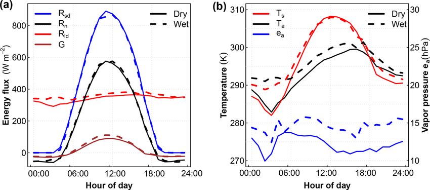
M. Renner et al.: Using phase lags to evaluate model biases in simulating the diurnal cycle of evapotranspiration                     519

Figure 2. Location of the EC site at Petit-Nobressart, Luxembourg. (a) shows the location within Western Europe. (b) shows an orthophoto of
the surroundings of the system (ESRI® World Imagery). (c) shows a picture of the mast with micrometeorological sensors. The soil sensors
are located on the right of the solar panel. Photo: Elisabeth Thiem.

tire period until 23 July. Table 1 lists the variables obtained         Table 1. Variables provided by the surface energy balance station
from the EC station and used in this work. For more details             and used for this work.
on instrumentation and EC data processing, see Ingwersen et
al. (2011) and Wizemann et al. (2015).                                       Variable                             Symbol     Unit
                                                                             Horizontal wind components           U, V       m s−1
2.2.1   Derived meteorological variables                                     Vertical wind                        w          m s−1
                                                                             Sensible heat flux                   H          W m−2
We derived the saturated water vapor pressure es (hPa) using
                                                                             Latent heat flux                     λE         W m−2
the empirical Magnus equation (Magnus, 1844) as a function
                                                                             Ground heat flux                     G          W m−2
of air temperature T (◦ C) with empirical coefficients from
                                                                             Upward shortwave radiation           Rsu        W m−2
Alduchov and Eskridge (1996):
                                                                             Incoming shortwave radiation         Rsd        W m−2
                                                                             Upward longwave radiation            Rlu        W m−2
es = 6.1094 · e(17.625·T /(243.04+T )) .
                                                                             Downward longwave radiation          Rld        W m−2
Then, the water vapor pressure of the air ea (hPa) was                       Friction velocity                    u∗         m s−1
                                                                             Air temperature                      Ta         K, ◦ C
obtained by using air temperature Ta and relative humid-
                                                                             Relative humidity                    RH         %
ity (RH):
                                                                             Surface air pressure                 p          hPa
                                                                             Precipitation                        P          mm
ea = es (Ta ) RH/100.
                                                                             Soil moisture (5, 15 and 30 cm)      θ          m3 m−3
                                                                             Soil temperature (5, 15 and 30 cm)   Tsoil      K
To assess the moisture conditions of each date of the site we
used the evaporative fraction fE :

fE = λE/(H + λE).

Since daily averages can be influenced by single large val-             where fE is the slope of the linear regression, β its intercept,
ues of the turbulent fluxes and contain missing values, we              and εR the residuals. Since we use the fluxes of H and λE
estimated a daily fE based on the 30 min values of each day             without energy balance closure correction, we obtain the up-
using the following linear regression:                                  per range of fE .
                                                                           Since the sonic anemometer measures friction veloc-
λE = fE (H + λE) + β + εR ,                                             ity (u∗ ) and the absolute value of wind speed u =

www.hydrol-earth-syst-sci.net/23/515/2019/                                               Hydrol. Earth Syst. Sci., 23, 515–535, 2019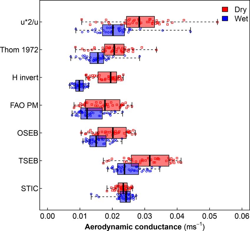
520     M. Renner et al.: Using phase lags to evaluate model biases in simulating the diurnal cycle of evapotranspiration
p
  (U 2 + V 2 ), we estimate the aerodynamic conductance for         2.3   One- and two-source energy balance models
momentum (u∗2 /u) and the aerodynamic conductance (gah )
for heat including the excess resistance to heat transfer using     Thermal-remote-sensing-based models estimate evapotran-
an empirical formula by Thom (1972):                                spiration by solving the surface energy balance and rely on
                                                                    land-surface temperature (Ts ) information as a key boundary
                      6.2 −1

                u                                                   condition (Kustas and Norman, 1999). A bulk layer formu-
gah,Thom =         +          .                             (5)
               u∗2 u∗ 23                                            lation of the soil-plus-canopy sensible heat flux is employed
                                                                    and λE is derived by enforcing the surface energy balance.
We chose to use this formula for its simplicity and similar         Hence λE is written as
performance than more recent, complex parameterizations
(Knauer et al., 2018; Mallick et al., 2016). Also note that         λE = Rn − G − H = Rn − G − ρcp (Ts − Ta ) gah ,                          (6)
effects of atmospheric stability are accounted for in the first     where ρ is the density of air, cp is the specific heat of air
term of Eq. (5).                                                    at constant pressure, and gah is the effective aerodynamic
                                                                    conductance of heat that characterizes the transport of sen-
2.2.2   Energy balance closure gap correction
                                                                    sible heat between the surface and the atmosphere. We ob-
Most EC measurements show that the sum of the observed              tained Ts from the observed longwave emission of the sur-
turbulent heat fluxes is smaller than the available energy and      face Ts = (Rlu /(σ εs ))1/4 with σ = 5.67 × 10⁻⁸ W K−4 (the
thus does not close the energy balance, leaving an energy           Stefan–Boltzmann constant) and a surface emissivity εs =
balance closure gap (Qgap ) (Foken, 2008):                          0.98, which is typical for a grassland and agrees with Bren-
                                                                    ner et al. (2017).
Qgap = Rn − (G + H + λE).                                              We use two different approaches which are generally clas-
                                                                    sified as one- and two-source models with regard to the im-
For our site we observed on average a slope of (H + λE) ∼           plemented treatment of the energy exchange with the sur-
(Rn − G) = 0.81 (by linear regression) with an average gap          face. While one-source energy balance models treat the sur-
of 37 W m−2 over the whole duration of the field campaign.          face as a uniform layer, two-source energy balance mod-
These values are in the typical range of what is commonly           els partition temperatures as well as radiative and energy
found for grassland sites (Stoy et al., 2013).                      fluxes into a soil and vegetation component. The one-source
   To correct the turbulent fluxes for the energy balance clo-      approach (OSEB) parameterizes the aerodynamic conduc-
sure gap (evaluated at the 30 min time steps), we use a cor-        tance gah as follows (e.g., Kalma et al., 2008; Tang et al.,
rection based on the Bowen ratio (BR ) (Twine et al., 2000),        2013):
which is directly related to the evaporative fraction fE =
1/(BR + 1) to obtain corrected fluxes:                              gah,OSEB =
                                                                                                   k2 u
λEBRC = λE + Qgap · fE
                                                                                                                                     ,   (7)
                                                                     ln ((zu − d) /z0m ) − 9m ln ((zt − d) /z0m ) + ln (z0m /z0h ) − 9h

and                                                                 where zu and zt are the measurement heights of wind and air
                                                                    temperature, respectively; z0m and z0h are roughness lengths
HBRC = H + Qgap · (1 − fE ) .                                       for momentum and heat, respectively; k is the von Kármán
                                                                    constant; d is the displacement height; u is the wind speed;
The correction is applied at 30 min time steps using the daily      and 9m and 9h are the the integrated Monin–Obukhov (MO)
fE estimates. We use these corrected fluxes in the further          similarity functions which correct for atmospheric stability
analysis.                                                           conditions (Brutsaert, 2005; Jiménez et al., 2012). For the
                                                                    investigated grassland site, d and z0m were calculated as
2.2.3   Clear-sky day classification
                                                                    fractions of the vegetation height, hc , with d = 0.65hc and
In order to achieve comparable conditions with respect to in-       z0m = 0.125hc . The roughness length for heat z0h was set us-
coming solar radiation, we identified clear-sky conditions. A       ing the dimensionless parameter kB −1 = ln(z0m /z0h ), which
clear-sky day was defined by its daily sum of incoming solar        was set to 2.3 in accordance with Bastiaanssen et al. (1998).
radiation being larger than 85 % of the potential surface radi-     Note that this parameterization of aerodynamic conductance
ation (Rsd,pot ), which is a function of latitude and day of year   does not explicitly distinguish between bare soil and canopy
(using R package REddyProc, function fCalcPotRadiation):            boundary layer conductance, as it is done in two-source ap-
                                                                  proaches.
Rsd /Rsd,pot > 0.856 (Rsd (t)) / fdiff 6 Rsd,pot (t) ,                 In addition to OSEB we applied the two-source energy
                                                                    balance model developed by Norman et al. (1995) and Kus-
where t corresponds to each time step of measurement and            tas and Norman (1999). For both the soil and canopy com-
with fdiff = 0.78 being a constant factor taking into account       ponents, a separate energy balance (with different compo-
atmospheric extinction of solar radiation.                          nent temperatures) and bulk resistance scheme with different

Hydrol. Earth Syst. Sci., 23, 515–535, 2019                                           www.hydrol-earth-syst-sci.net/23/515/2019/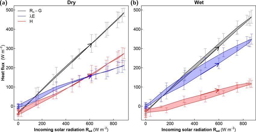
M. Renner et al.: Using phase lags to evaluate model biases in simulating the diurnal cycle of evapotranspiration               521

aerodynamic conductance are formulated. Then the energy             on a sub-daily scale. In order to understand the effect of the
balance equations are solved iteratively. It starts by assuming     aerodynamic conductance parameterizations we add another
that a fraction of the canopy (described by vegetation green-       reference evapotranspiration estimate in which the aerody-
ness fraction fg ) transpires at a potential rate as described by   namic conductance is given by Eq. (5) using observations of
the Priestley–Taylor equation (Priestley and Taylor, 1972):         friction velocity and wind speed, but keeping gs fixed.
               s                                                    Penman–Monteith-based Surface Temperature Initiated
λEPT = αPT        (Rn − G) ,                                 (8)
             s +γ                                                   Closure (STIC) (version STIC1.2)
where αPT is the Priestley–Taylor coefficient (1.26), s is the      In order to estimate an actual evapotranspiration rate from
slope of the saturation water vapor pressure curve, and γ is        meteorological data we employ a method (STIC1.2 hereafter
the psychrometric constant. However, the canopy latent heat         referred to as STIC), which is based on the PM equation,
flux λEc = fg λEPT might be too large and the soil compo-           but which in addition integrates surface temperature infor-
nent would become negative (condensation at the soil sur-           mation. The STIC methodology is based on finding analyti-
face), which is unlikely during daytime conditions. To avoid        cal solutions for the two unknown conductances to directly
condensation at the soil surface, the αPT coefficient is re-        estimate λE (Mallick et al., 2016, 2018). STIC is a one-
duced incrementally until the soil latent heat flux becomes         dimensional physically based surface energy balance model
zero or positive. Once this condition is met, all other energy      that treats the vegetation–substrate complex as a single unit
balance components are updated accordingly to satisfy the           (Mallick et al., 2016; Bhattarai et al., 2018). The fundamen-
energy balance equation. For this study we used a constant          tal assumption in STIC is the first-order dependency of ga
vegetation fraction of fc = 0.9 and a greenness fraction fg         and gs on soil moisture through Ts and on environmental
which was derived from close-up pictures taken at the begin-        variables through Ta , Da , and net radiation. Therefore, sur-
ning and the end of the field campaign and linearly interpo-        face temperature is assumed to provide information on water
lated in-between.                                                   limitation which is linked to the advection–aridity hypothesis
                                                                    (Brutsaert and Stricker, 1979). In STIC, no wind speed is re-
2.4   Penman–Monteith approach
                                                                    quired as input data, as opposed to the temperature-gradient
In the Penman–Monteith approach (Monteith, 1965) the in-            approaches, but vapor pressure of the air and its saturation
clusion of physiological conductance (gs ) imposes a critical       value become critical input variables; see Table 2 for an
control on λE:                                                      overview. A detailed description of STIC version 1.2 is avail-
                                                                    able in Mallick et al. (2016, 2018) and Bhattarai et al. (2018).
       s (Rn − G) + ρcp gav (es (Ta ) − ea )
λE =                                       .               (9)
                s + γ 1 + ggavs                                     3     Results
In Eq. (9), the transfer of moisture is linked to a supply–         3.1    Daily clear-sky and moisture classification
demand reaction where the net available energy (Rn − G)
is the supply energy for evaporation and the vapor pres-            The field campaign was conducted during an exceptionally
sure deficit of the air Da [= es (Ta ) − ea ] is the demand for     warm and dry period characterized by clear-sky conditions
evaporation from the atmosphere. In the PM approach, the            with remarkably high air temperatures with daily maxima
two conductances, the aerodynamic conductance gav and               above 30 ◦ C and little precipitation. Compared to the cli-
the surface conductance gs , to water vapor are unknown. A          matic normal (1981–2010) the precipitation deficit in this
widely used approach to obtain a reference evapotranspira-          region was −44 % in June and −41 % in July, respectively
tion estimate from meteorological data is the FAO Penman–           (source: meteorological station Arsorf, Administration des
Monteith reference evapotranspiration (Allen et al., 1998). It      services techniques de l’agriculture – ASTA). The air tem-
defines the two conductances for a well-watered grass sur-          perature anomaly was higher in July (1.9 ◦ C) than in June
face with a standard height of h = 0.12 m. The aerodynamic          (0.7 ◦ C) (source: meteorological station Clemency, ASTA).
conductance is obtained by a bulk approach (Eq. 7) with             The soil water content decreased and parts of the site, espe-
wind speed u measured at 2 m above the surface, d = 2/3h,           cially the upper part, showed clear signs of vegetation water
z0m = 0.123h, z0h = 0.1z0m , yielding gav = u/208 (Box 4 in         stress (see Brenner et al., 2017, for an analysis of the spatial
Allen et al., 1998). Surface conductance is fixed at a constant     heterogeneity of water limitation). However, the dry period
gs = 1/70 m s−1 . Here, we use the latter definitions of the        was interrupted by a few but strong rainfall events, which
conductances and use direct measurements for the other in-          significantly changed soil moisture and thus fE with time
put variables of Eq. (9) to obtain the FAO Penman–Monteith          (Fig. 3a). Based on the observed fE we classified dry days
estimate. While the FAO estimate is typically intended for          with fE < 0.5 and wet days with fE > 0.6. This separation
estimates of the reference evaporation for well-watered grass       of dry and wet days is also reflected in the top soil moisture
on a daily basis, we use it here as a reference for comparison      conditions (measured at 5 cm depth) as shown in Fig. 3b.

www.hydrol-earth-syst-sci.net/23/515/2019/                                          Hydrol. Earth Syst. Sci., 23, 515–535, 2019
522    M. Renner et al.: Using phase lags to evaluate model biases in simulating the diurnal cycle of evapotranspiration

Table 2. Input variables used in the different evapotranspiration schemes.

      Scheme                                   Rn      G      Ta     Ts         ea       es     u    Other parameters
      Priestley–Taylor                        Obs     Obs    Obs
      Penman–Monteith (with constant gs )     Obs     Obs    Obs             Obs        Obs    Obs   gah,Thom = f (u, u∗ ) (5), gs = const
      FAO Penman–Monteith                     Obs     Obs    Obs             Obs        Obs    Obs   gav = u/208, gs = 1/70 m s−1
      OSEB                                    Obs     Obs    Obs    Obs                        Obs   hc
      TSEB                                    Obs     Obs    Obs    Obs                        Obs   fc , fg , hc
      STIC                                    Obs     Obs    Obs    Obs      Obs        Obs

Figure 3. Daily observations of soil moisture, evaporative fraction, ratio of observed to potential solar radiation, and mean precipitation.
(a) shows the daily time series and (b) the relationship of fE to soil moisture used to classify wet and dry days depending on fE > 0.6 or
fE < 0.5, respectively. Sunny days are defined using a threshold of 85 % of Rsd to potential radiation and are marked with solid symbols,
with blue circles referring to wet days and red squares to dry days. Top soil moisture measured at 5 cm below surface is shown.

   Based on the classification of wet and dry days under                  3.2        Diurnal cycle of evapotranspiration under wet and
clear-sky conditions we computed composites of the diur-                             dry conditions
nal cycle for each hour. By using only sunny days we aim
to achieve similar conditions with respect to downwelling                 Next, we evaluate how the different evapotranspiration
shortwave radiation (Rsd ). Figure 4a confirms that Rsd and               schemes are able to reproduce the fluxes during wet and dry
net radiation (Rn ) had very similar diurnal cycles and mag-              conditions under similar Rsd forcing. Figure 5 shows the av-
nitudes for the wet and dry days. However, the downwelling                erage diurnal cycle of observations and models for λE. The
longwave radiation Rld and the soil heat flux were somewhat               observations showed a significant difference in λE between
higher under wet conditions (Fig. 4a). The higher Rld is re-              dry and wet conditions, with a maximum value of λE of
lated to higher air temperatures and air vapor pressures ob-              about 200 W m−2 for dry and 350 W m−2 under wet con-
served under wet conditions (Fig. 4b), which may explain the              ditions, which amounts to a mean difference of 100 W m−2
greater value of Rld by affecting the atmospheric emissivity              for daylight conditions (Table 3). As reference, we also in-
for longwave radiative exchange. This has also an impact on               cluded two common formulations of potential evapotranspi-
the minimum temperatures both for air and skin temperature,               ration, the Priestley–Taylor potential evapotranspiration (PT)
which are higher under wet conditions and lower under dry                 and the FAO Penman–Monteith reference evapotranspira-
conditions (Fig. 4b). Hence, although we achieve fairly simi-             tion (FAO-PM). Both do not account for water limitation and
lar conditions for shortwave radiation under wet and dry con-             show a marginal difference of 10 W m−2 between wet and
ditions, we observed a small but significant difference in the            dry conditions. While FAO-PM yielded lower mean condi-
longwave radiative exchange.                                              tions than PT, it showed lower correlation and RMSE as com-
                                                                          pared to PT (Table 3). We find that all models for actual λE
                                                                          (rather than PT or FAO-PM) showed differences in λE be-
                                                                          tween wet and dry conditions. Both OSEB and TSEB showed
                                                                          a tendency to overestimate λE under dry conditions but cap-
                                                                          tured the high λE values under wet conditions. In contrast,

Hydrol. Earth Syst. Sci., 23, 515–535, 2019                                                   www.hydrol-earth-syst-sci.net/23/515/2019/
M. Renner et al.: Using phase lags to evaluate model biases in simulating the diurnal cycle of evapotranspiration                           523

Figure 4. Observations of average diurnal cycles of energy fluxes (a), with Rsd representing the shortwave downwelling flux, Rld the
longwave downwelling flux, Rn the net radiation, G the ground heat flux, Ts and Ta the surface and air temperatures, and ea the air vapor
pressure, comparing wet and dry days (b).

Table 3. Statistics for all days and sunny wet or dry days based on 30 min values during daytime hours 06:00–18:00 LT. Performance
statistics, root mean square error (RMSE), and explained variance r 2 are computed with respect to the observed latent heat flux corrected for
the closure gap by the Bowen ratio (λEBRC ). As a reference we also provide statistics for the uncorrected, observed latent heat flux (λEuncor ).
Potential evapotranspiration estimates are Priestley–Taylor (PT) and FAO Penman–Monteith (FAO-PM) reference evapotranspiration. Actual
λE estimates are provided by the three schemes. Statistics are computed for all days and for clear-sky days classified as wet and dry.

                          Statistic   Period    λEBRC       λEuncor      PT    FAO-PM       OSEB      TSEB      STIC
                          Mean        all           178         145     259          224       202       204      170
                          Mean        wet           264         213     325          294       255       259      218
                          Mean        dry           164         134     315          285       212       209      180
                          RMSE        all              0         40     106           81        41        43       46
                          RMSE        wet              0         57      71           52        29        24       66
                          RMSE        dry              0         33     169          140        57        58       45
                          r2          all           1.00       0.94    0.72         0.62      0.85      0.84     0.72
                          r2          wet           1.00       0.91    0.96         0.83      0.92      0.92     0.66
                          r2          dry           1.00       0.93    0.75         0.56      0.62      0.61     0.44

STIC captured the low λE magnitude under dry conditions                    whereas STIC showed relatively higher RMSE. However,
(fE < 0.5) but underestimated λE under wet conditions (for                 under dry conditions the RMSE of OSEB–TSEB models was
fE > 0.6).                                                                 found to be larger than for STIC. For the entire observation
   Table 3 shows the statistical metrics of the model per-                 period the three models produced comparable RMSE (41–
formances with respect to the Bowen-ratio-corrected λE.                    46 W m−2 ) but with different correlation. STIC produced rel-
In general, both OSEB and TSEB produced mean λE val-                       atively low correlation (r 2 = 0.72) as compared to the other
ues within the range of 96 %–98 % (255 and 259 W m−2 )                     two models (r 2 = 0.84–0.85). Therefore, we find that the
of the observed λE (264 W m−2 ) in wet conditions, while                   correlation of the schemes is distinctly larger under wet con-
mean λE from STIC was within 83 % (218 W m−2 ) of ob-                      ditions as compared to dry conditions. The correlations un-
served λE for the same conditions. However, for the dry                    der wet conditions of OSEB and TSEB are in the range of the
conditions, simulated λE from STIC (180 W m−2 ) was 91 %                   correlation of the uncorrected λE (r 2 = 0.91), whereas STIC
of the observed mean λE (164 W m−2 ), while the simu-                      and FAO-PM showed lower correlation. Under dry condi-
lated mean λE from OSEB and TSEB was 77 %–78 % of                          tions the correlation was significantly lower than the correla-
the observed mean λE. Overall, the three models captured                   tion of the uncorrected λE (r 2 = 0.93). While OSEB–TSEB
86 % (OSEB), 88 % (TSEB), and 95 % (STIC) of the ob-                       explained 62 % of the observed uncorrected λE variability
served mean λE. Results show that, under wet conditions,                   in dry conditions (STIC explained 44 %), both models pro-
RMSE of the OSEB–TSEB models is well within the range                      duced higher RMSE (57–58 W m−2 ) as compared to STIC
of the errors when compared with the uncorrected λE,                       (45 W m−2 ) under these conditions.

www.hydrol-earth-syst-sci.net/23/515/2019/                                                  Hydrol. Earth Syst. Sci., 23, 515–535, 2019
524    M. Renner et al.: Using phase lags to evaluate model biases in simulating the diurnal cycle of evapotranspiration

Figure 5. Average diurnal cycle of λE estimates for (a) dry and (b) wet days. Error bars denote the standard deviation obtained for each
hour. The bold black line with squares shows the observed latent heat flux corrected for the surface energy balance closure (λEBRC ). The
grey-shaded area depicts the range induced by the energy balance closure gap.

Figure 6. Diurnal hysteresis of λE to Rsd for (a) dry and (b) wet conditions of observations and different models. Bold arrows indicate the
rising limb in the morning hours (07:00 to 08:00 LT) showing a counterclockwise hysteresis of λE under wet conditions. Vertical arrows
depict the standard deviation of λEBRC for each hour.

3.3   Diurnal patterns of evapotranspiration                               The two potential evapotranspiration estimates showed
                                                                        large differences in their phase lag. While the PT estimate
The evaluation of the diurnal cycle shows that λE was                   showed a small hysteretic loop with a phase lag between
strongly related to the incoming solar radiation, emphasiz-             tϕ = 6–9 min, the FAO-PM estimate showed a substantial
ing that Rsd is the dominant driver of λE (Fig. 6). However,            loop with a phase lag of tϕ = 31 min. This large phase lag of
under wet conditions we found a marked and consistent dif-              the FAO-PM estimate is very similar to the phase lag when
ference between morning and afternoon in λE, forming a                  we use a constant gs in the PM equation but with gav ob-
CCW hysteresis loop (Fig. 6b). Using the Camuffo–Bernardi               tained from Eq. (5) using friction velocity observations (Ta-
regression we found a significant phase lag for the Bowen-              ble 4). The temperature-gradient schemes (OSEB and TSEB)
ratio-corrected flux (λEBRC ) with a mean tϕ = 15 min under             reproduced the observed phase lag relatively well (mean tϕ =
wet conditions and no significant lag under dry conditions              9 min for wet and around 0 for dry conditions). However, the
(Fig. 7 and Table 4). The uncorrected observations showed               temperature- and vapor-gradient scheme (STIC) showed rel-
only a slightly lower wet–dry difference, highlighting that             atively larger phase lags under both dry and wet conditions
the method to close the energy balance closure gap does not             (tϕ = 14–20 min) (Fig. 7, Table 4).
significantly influence the estimated phase lag.

Hydrol. Earth Syst. Sci., 23, 515–535, 2019                                             www.hydrol-earth-syst-sci.net/23/515/2019/
M. Renner et al.: Using phase lags to evaluate model biases in simulating the diurnal cycle of evapotranspiration 525
Table 4. Results of the Camuffo–Bernardi regression model with mean (standard deviation) for wet and dry days. The slope of the variable
against Rsd is represented by b (note that the unit of b depends on the unit of the variable) and the phase lag to incoming solar radiation is
converted to minutes. The adjusted explained variance by the multilinear regression model is given in column r 2 . The phase lag to Rn − G is
reported in the last column for comparison.
Variable Moisture Slope b Phase lag to r 2 adjusted Phase lag to
conditions Rsd (in min) Rn − G (in min)
wet 0.7162 (0.0106) 1 (3) 0.998 −2 (2)
Net radiation
dry 0.6980 (0.0119) −1 (2) 0.998 0 (1)
wet 0.1483 (0.0194) −6 (8) 0.964 −8 (9)
Soil heat flux
dry 0.1261 (0.0173) −0 (8) 0.968 2 (7)
wet 0.5679 (0.0122) 3 (3) 0.998 –
Available energy
dry 0.5719 (0.0180) −1 (2) 0.998 –
wet 0.1715 (0.0275) −22 (6) 0.964 −25 (7)
Sensible heat flux
dry 0.3388 (0.0470) −3 (8) 0.988 −3 (8)
wet 0.0340 (0.0092) 133 (84) 0.600 124 (77)
Incoming longwave
dry 0.0263 (0.0115) 176 (51) 0.459 158 (49)
wet 0.3992 (0.0186) 15 (4) 0.990 11 (3)
λEBRC
dry 0.2380 (0.0317) 3 (12) 0.981 3 (11)
wet 0.3284 (0.0289) 14 (5) 0.967 10 (4)
λEuncor
dry 0.1939 (0.0271) 2 (16) 0.963 3 (14)
wet 0.5354 (0.0279) 9 (5) 0.997 5 (2)
Priestley–Taylor
dry 0.5238 (0.0414) 6 (4) 0.996 6 (3)
wet 0.4326 (0.0371) 30 (9) 0.981 25 (6)
Penman–Monteith constant gs
dry 0.4288 (0.0456) 35 (11) 0.974 32 (10)
wet 0.4233 (0.0432) 31 (11) 0.980 26 (9)
FAO Penman–Monteith
dry 0.4200 (0.0533) 31 (12) 0.981 29 (12)
wet 0.3718 (0.0100) 9 (6) 0.976 5 (4)
λE OSEB
dry 0.2978 (0.0372) −2 (5) 0.948 −1 (5)
wet 0.3793 (0.0228) 9 (5) 0.989 5 (2)
λE TSEB
dry 0.2843 (0.0545) 1 (6) 0.962 1 (4)
wet 0.3037 (0.0695) 20 (19) 0.876 15 (19)
λE STIC
dry 0.2387 (0.0655) 14 (14) 0.892 13 (12)
wet 0.0088 (0.0008) 130 (41) 0.742 122 (41)
Air temperature
dry 0.0084 (0.0017) 138 (35) 0.685 130 (37)
wet 0.0203 (0.0010) 51 (18) 0.923 46 (16)
Surface temperature
dry 0.0228 (0.0027) 51 (13) 0.933 49 (13)
wet 0.0116 (0.0013) −22 (8) 0.966 −24 (10)
Ts − Ta
dry 0.0145 (0.0017) −10 (7) 0.973 −7 (7)
wet 0.0003 (0.0015) 127 (186) 0.266 115 (183)
Vapor pressure
dry −0.0003 (0.0012) 52 (246) 0.316 71 (250)
wet 0.0143 (0.0031) 145 (39) 0.791 134 (40)
Vapor pressure deficit
dry 0.0128 (0.0032) 153 (46) 0.719 144 (47)
www.hydrol-earth-syst-sci.net/23/515/2019/ Hydrol. Earth Syst. Sci., 23, 515–535, 2019526 M. Renner et al.: Using phase lags to evaluate model biases in simulating the diurnal cycle of evapotranspiration
with a triangular shape with higher values during the after-
noon when solar radiation reduces. Interestingly, the surface-
to-air temperature gradient, being the driving gradient for the
sensible heat flux, showed much lower hysteretic behavior.
The hysteresis is in a clockwise direction, with a higher gra-
dient in the morning hours compared to the afternoon. It had
a similar phase lag to H (see Table 4).
We further analyzed different formulations of the aerody-
namic conductance (ga ) directly inferred from measurements
and from how these are represented in the models evalu-
ated here (FAO-PM, OSEB, TSEB, STIC). We inferred the
aerodynamic conductance from observations in three differ-
ent ways: firstly, we used the eddy-covariance measurements
of friction velocity (u∗ ) and wind speed (u) to estimate the
aerodynamic conductance for momentum (gam = u∗2 /u). We
then used the empirical formula by Thom (1972) to calculate
the aerodynamic conductance for heat including the excess
Figure 7. Boxplot of the daily phase lag of λE to Rsd for observed
resistance to heat transfer (Eq. 5). Thirdly, we inferred the
(without and with Bowen ratio correction) and modeled latent heat
aerodynamic conductance from the observed sensible heat
flux using sunny dry (red) and wet (blue) days. A positive phase
lag means that λE follows Rsd and thus forms a CCW hysteresis flux (HBRC ) and temperature gradient (Ts − Ta ) by invert-
as shown in Fig. 6. Dots show the actual data for each day with ing HBRC using Eq. (6). The FAO-PM describes the aerody-
filled symbols indicating significant phase lags (P < 0.05, t test of namic conductance with a simple linear relationship to wind
coefficient significantly different from 0). speed. OSEB and TSEB estimates the aerodynamic conduc-
tance to heat (gah ), while STIC estimates the conductance to
water vapor (gav ). Thus by comparing these different con-
Since all evapotranspiration schemes use Rn − G as forc- ductance estimates we assume similarity between the fluxes.
ing, we also computed the phase lags with Rn − G as a ref- The different estimates for the aerodynamic conductance
erence variable (see Table 4). The differences to Rsd as ref- are compared to each other in Fig. 10 for midday conditions.
erence are, however, rather small with slightly lower phase Although the three observation-based estimates show some
lags and in the range of the standard deviation of the daily variations in the absolute value of the aerodynamic conduc-
estimates. This small difference can be attributed to a neg- tance, they consistently showed a significantly greater con-
ligible phase lag between Rsd and Rn as well as the rather ductance for dry days compared to wet days, suggesting a
small magnitude and the phase lag of the soil heat flux. stronger aerodynamic exchange between the surface and the
atmosphere under dry conditions. This difference in aerody-
3.4 Diurnal patterns of observed fluxes and states namic conductance is partly reproduced by the simple FAO-
PM scheme, which means that the median wind speed was
In order to understand the diurnal patterns of λE we also ana- higher under the drier conditions. The temperature-gradient
lyzed the hysteresis loops of the observed surface energy bal- schemes (OSEB and TSEB) reproduce the wet–dry differ-
ance components [λE = (Rn − G) − H ] with respect to Rsd ence rather well, and they also use wind speed but rely on
(Fig. 8). Generally, there was only a small hysteresis in the Monin–Obukhov similarity theory and stability correction.
available energy (Rn −G) (Table 4). The turbulent heat fluxes STIC, which does not use wind speed, did not show any sig-
showed significant hysteresis under wet conditions but not nificant differences in gav between wet and dry conditions.
under dry conditions. Interestingly, under wet conditions the Finally we analyze the diurnal patterns of the vapor pres-
CCW hysteresis of λE with a phase lag (mean tϕ = 15 min) sure deficit Da = es (Ta ) − ea , which is a critical driver of the
was mostly compensated for by a CW hysteresis of H (mean latent heat flux in the PM equation. Since Da is derived from
tϕ = −22 min) (Fig. 8 and Table 4). This compensation is an the observations, we analyzed its diurnal patterns in Fig. 11.
outcome of net available energy (Rn − G) showing little hys- We found that the vapor pressure in the air remained fairly
teresis for both conditions. constant during the day; hence it did not co-vary with Rsd and
We next analyzed the bulk sensible heat flux formulation only showed a small CW hysteresis with higher vapor pres-
used in the OSEB and TSEB models to understand how the sure during the morning compared to during the afternoon.
observations of temperature and the inferred aerodynamic The saturation vapor pressure, which is a function of air tem-
conductances are related to each other. The diurnal patterns perature, however, showed a distinct and large CCW hystere-
of both air and surface temperature revealed a strong CCW sis loop with respect to Rsd , which is consistent with the large
hysteresis with Rsd (Fig. 9). Air temperature showed a more hysteresis in air temperature (Figs. 9 and 12). As a conse-
pronounced hysteretic loop than surface temperature, and quence, Da also showed a distinct and large CCW hysteresis
Hydrol. Earth Syst. Sci., 23, 515–535, 2019 www.hydrol-earth-syst-sci.net/23/515/2019/M. Renner et al.: Using phase lags to evaluate model biases in simulating the diurnal cycle of evapotranspiration 527
Figure 8. Diurnal patterns of observed surface energy balance components for (a) dry and (b) wet days. The lines show the composite
average and vertical bars the standard deviation for available energy (black), latent heat (blue), and sensible heat (red) of each hour. There is
a nearly linear response of all surface heat fluxes to Rsd under dry conditions and a systematic hysteresis loop under wet conditions. Under
wet conditions the CCW hysteresis of λE is mostly compensated for by a CW hysteresis of H .
Figure 9. Diurnal patterns of observed anomalies in surface temperature (Ts ), air temperature at 2 m (Ta ), and their gradient (Ts − Ta ) for
(a) dry and (b) wet days. Both Ta and Ts show a pronounced CCW hysteresis, but the form of the hysteretic loop is significantly different,
with air temperature featuring a more pronounced, triangular shape with afternoon values almost independent of incoming solar radiation.
The temperature gradient, however, shows a much smaller CW hysteretic loop. Note that the temperature gradient is comparatively higher in
the morning than in the afternoon, corresponding to the diurnal course of the sensible heat flux (see Fig. 8).
with a large phase lag of tϕ =∼ 150 min (see Table 4). This 4 Discussion
large hysteresis and phase lag is consistent with the respec-
tive characteristics of air temperature, but not with those of 4.1 Dominant controls of λE at the diurnal cycle
the temperature gradient (see Fig. 9). Furthermore, we note
that the phase lag in Da did not show any significant influ- Our analysis of the diurnal cycle showed that λE follows the
ence of wetness, while the phase lag of the temperature gra- diurnal course of incoming solar radiation, explaining most
dient became more negative under wet conditions (Fig. 12, of the variance in λE. However, a significant nonlinearity in
Table 4). It would thus seem that the bias in PM-based es- the form of a phase lag between λE and Rsd was detected,
timates identified here may relate to a too-pronounced role which showed larger λE for the same Rsd in the afternoon
of Da in the evapotranspiration estimate. as in the morning. We found that the lag in λE is accom-
panied by a preceding phase lag of the sensible heat flux,
while the other surface energy balance components (e.g., net
www.hydrol-earth-syst-sci.net/23/515/2019/ Hydrol. Earth Syst. Sci., 23, 515–535, 2019528 M. Renner et al.: Using phase lags to evaluate model biases in simulating the diurnal cycle of evapotranspiration
The obtained phase lags of the surface fluxes and variables
allow for a process-based insight into the diurnal heat ex-
change of the surface with the atmosphere. Since there is
only limited heat storage in the surface layer itself, which
explains the small phase lags of the heat fluxes, the heat-
ing imbalance caused by solar radiation must be effectively
redistributed. Over land it is the lower atmosphere which
acts as efficient heat storage to buffer most of the diurnal
imbalance caused by solar radiation, because the heat stor-
age of the subsurface is limited by the relatively slow heat
conduction into the soil. Thus, the lower atmosphere is ef-
fectively heated by surface longwave emission and the sen-
sible heat flux, which in combination with the diurnal cy-
cle of vertically transported turbulent kinetic energy (TKE)
leads to the development of the convective planetary bound-
ary layer (CBL) (e.g., Oke, 1987). The changes in heat stor-
age in the CBL are reflected by the very large phase lags for
air temperature and longwave downwelling radiation, which
both have a phase lag of about 2.5 h. This large phase lag
Figure 10. Boxplot of the different estimates of aerodynamic con- of air temperature then shapes (i) the vertical surface-to-air
ductance under dry (red) and wet (blue) conditions. Only sunny temperature gradient, which drives the sensible heat flux; and
days are sampled and midday values (10:00–15:00 LT) are used in (ii) the vapor pressure deficit of the air. Despite the complex-
the comparison. The top three estimates are directly inferred from ity of processes within the convective boundary layer, includ-
observations, as described in the text. ing the morning transition and entrainment at its top, we find
that all surface energy components correlate strongly with
solar radiation (Table 4). What this suggests is that the state
radiation and soil heat flux) revealed very small phase lags of the surface–atmosphere system is predominantly shaped
with Rsd . Hence, there is compensation between the phase by fluxes, particularly by solar radiation as its primary driver,
shifts of sensible and latent heat fluxes, which becomes more with the state in terms of temperatures and humidity gradi-
apparent under the wet conditions. Our results are consis- ents adjusting to these fluxes, rather than the reverse, where
tent with the comprehensive FLUXNET studies of Wilson et the state (in terms of temperature and humidity) drives the
al. (2003) and Nelson et al. (2018) which used a different fluxes.
metric (median centroid) for assessing diurnal phase shifts. We also found that the phase lag of the turbulent heat
Wilson et al. (2003) found that H precedes λE at most sites, fluxes is affected by soil water availability. This is most
with the exception of sites in a Mediterranean climate. Using clearly seen for the surface-to-air temperature gradient and
the FLUXNET2015 dataset, Nelson et al. (2018) found that the sensible heat flux, whose phase lag is 2 times larger for
the median centroid of λE occurs predominantly in the after- wet than for dry days. This means that for the same solar
noon across all plant functional types when fE > 0.35, while radiation forcing we find higher values of the sensible heat
for very dry conditions (fE < 0.2) a shift of the λE cen- flux in the morning than in the afternoon. The effect of water
troid towards the morning was found. This indicates that availability is also seen for the phase lag of the latent heat
our results are not just applicable to Luxembourg, but are flux and to a lesser extent for the soil heat flux.
a general phenomenon which justifies a wider interpretation Our findings agree well with studies which use the diurnal
within temperate climates. centroid method, showing that moisture limitation decreases
It is important to emphasize here that the observed phase the lag in timing of λE (Wilson et al., 2003; Xiang et al.,
lags are not dominated by diurnal heat storage changes be- 2017; Nelson et al., 2018). The phase shift of Da might en-
low the surface, since both the diurnal magnitude and the hance evaporation at the cost of the sensible heat flux during
phase lag of the soil heat flux were relatively small compared the afternoon under sufficient moisture availability. However,
to the turbulent heat fluxes. The models employed here use under drier conditions, our findings suggest that the surface
available energy (Rn − G) as input to estimate λE. However, heats more strongly and generates more buoyancy, which is
the phase lag of the latent heat flux would only reduce by reflected by higher aerodynamic conductances as compared
about 3 min when choosing Rn − G instead of Rsd as the ref- to the wet conditions (Fig. 10). The larger aerodynamic con-
erence variable to calculate the phase lags. Hence, the ob- ductance would then enable a more effective sensible heat
served phase lags of λE and H to Rsd are not an artifact of exchange and would thus lower the phase difference between
the analysis, but can be considered as an imprint of L–A in- the sensible and latent heat fluxes.
teraction.
Hydrol. Earth Syst. Sci., 23, 515–535, 2019 www.hydrol-earth-syst-sci.net/23/515/2019/You can also read